List-based Interpretable Dynamic Treatment Regimes.

(1)

ABSTRACT

ZHANG, YICHI. List-based Interpretable Dynamic Treatment Regimes. (Under the direction of Dr. Eric B. Laber and Dr. Marie Davidian.)

Precision medicine is currently a topic of great interest in clinical and intervention science. It is well recognized as a path to delivering better healthcare while reducing cost, resource consumption, and treatment burden. A key component of precision medicine is that it is evidence-based, i.e., data-driven, and consequently there has been tremendous interest in estimation of precision medicine strategies using observational or randomized study data. One way to formalize precision medicine is to use a sequence of decision rules, one per stage of clinical intervention, that map up-to-date patient information to a recommended treatment. An optimal regime is defined as optimizing the mean of some cumulative clinical outcome if applied to a population of interest. It is well-known that even under simple generative models the optimal treatment regime can be a highly nonlin-ear function of patient information. Consequently, a focal point of recent methodological research has been the development of flexible models for estimating optimal treatment regimes. However, in many settings, estimation of an optimal treatment regime is an ex-ploratory analysis intended to generate new hypotheses for subsequent research and not to directly dictate treatment to new patients. Also, the development of treatment regimes for application in clinical practice requires the long-term, joint effort of statisticians and clinical scientists. In such settings, an estimated treatment regime that is interpretable in a domain context may be of greater value than an unintelligible treatment regime built using “black-box” estimation methods.

(2)

(3)

(4)

List-based Interpretable Dynamic Treatment Regimes

by Yichi Zhang

A dissertation submitted to the Graduate Faculty of North Carolina State University

in partial fulfillment of the requirements for the Degree of

Doctor of Philosophy

Statistics

Raleigh, North Carolina 2016

APPROVED BY:

Dr. Anastasios Tsiatis Dr. Leonard A. Stefanski

Dr. Eric B. Laber

Co-chair of Advisory Committee

(5)

BIOGRAPHY

(6)

ACKNOWLEDGEMENTS

I would like to express my sincere gratitude to my advisors Dr. Eric B. Laber, Dr. Marie Davidian and Dr. Anastasios Tsiatis for their valuable guidance during my PhD journey, which will also have an ongoing impact on my future career.

I would like to thank my committee member Dr. Leonard A. Stefanski for his insightful comments. I would also like to thank the professors in the department for their interesting and thought-provoking lectures.

I would like to thank my parents Quanxin Zhang and Yinian Liang for their constant love and support through my life.

(7)

LIST OF TABLES

Table 1.1 The second column gives the number of treatment options m. The third column gives the set ofφ functions used in the outcome mod-els. The fourth column specifies the form of the optimal regime πopt_{(x) = arg max}

aφ(x, a) where: “linear” indicates that πopt(x) =

arg maxa{(1, xT)βa} for some coefficient vectors βa ∈ Rp+1, a ∈ A;

“decision list” indicates thatπopt is representable as a decision list; and “nonlinear” indicates that πopt_{(x) is neither linear nor} repre-sentable as a decision list. . . 18 Table 1.2 The average value and the average cost of estimated regimes in

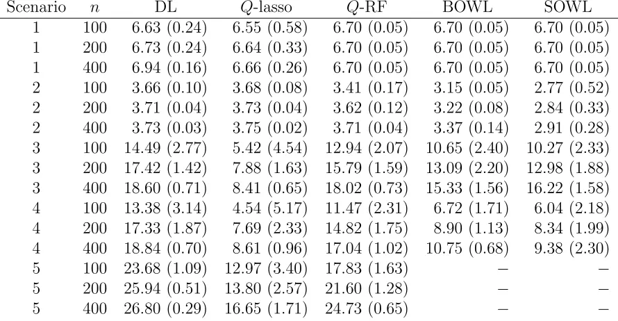
sim-ulated experiments. In the header, p is the dimension of patient covariates; DL refers to the proposed method using decision list; Q1 refers to parametric Q-learning; Q2 refers to nonparametric Q-learning; OWL1 and OWL2 refer to outcome weighted learning with linear kernel and Gaussian kernel, respectively; MCA refers to mod-ified covariate approach with efficiency augmentation. OWL and MCA are not applicable under Setting V, VI and VII. . . 19 Table 2.1 Simulation results. Given a scenario and a sample size, each method

constructed 1000 DTRs, one per each simulated dataset. The num-ber in each cell is the outcome under the estimated DTR, averaged over 1000 replications, with standard deviation in parentheses. In the header, n is the sample size, DL refers to the proposed deci-sion list based approach, Q-lasso refers to the Q-learning approach with linear model and lasso penalty,Q-RF refers to the Q-learning approach using random forest . . . 51 Table A.1 Point estimate and coverage probabilities of prediction intervals with

and without bootstrap bias correction. Plain-PI refers to the cov-erage probability of the plain prediction interval, and Corrected-PI refers to the coverage probability of the bias-corrected prediction interval. . . 95 Table A.2 Accuracy of variable selection using decision list. TPR is the true

(10)

Table A.3 The impact of α on the value and the cost of the estimated regime. In the header, α is the tuning parameter in the stopping criterion; R(_bπ) is the mean outcome under the estimated regimeπ, computed_b on a test set of 106 _subjects; _N₍

b

π) is the cost of implementing the estimated regimeπ, computed on the same test set; TPR is the true_b positive rate, namely, the number of signal variables involved in _bπ divided by the number of signal variables; FPR is the false positive rate, namely, the number of noise variables involved in _bπ divided by the number of noise variables. Recall that p is the dimension of patient covariates. . . 99 Table A.4 The impact of α on the estimated regime. In the header, α is the

tuning parameter in the stopping criterion and _bπα is the regime

such obtained. For each pair of regimes _bπα and bπα0, we report the probability that they recommend the same treatment for a ran-domly selected patient in the population. Mathematically, this is to compute Pr{π_bα(X) = bπα0(X)|πbα,bπα0} and then average over 1000 replications, where X is generated in the same way as in Section 3 in the main paper. . . 100 Table A.5 Consistency of the decision list. In the header, n is the sample size;

p is the number of predictors. Loss is R(πopt₎₋_R( b

π), namely, the difference between the the value under the estimated regime and the value under the optimal regime. Pr(best) is Pr{_bπ(X) =πopt(X)|_bπ}, namely, the probability that the treatment recommended by the es-timate regime coincides with the treatment recommended by the op-timal regime. Loss and Pr(best) are averaged over 1000 replications. Correct is the proportion of _bπ having the same form and covariates asπopt _{among 1000 replications; MSE}

(11)

LIST OF FIGURES

Figure 1.1 Estimated decision list for treating patients with chronic depression. 5 Figure 1.2 Left: diagram of a decision list dictated by regionsR1 ={x∈R2 : x1 > τ1},

R2 ={x∈R2 :x1 ≤τ1, x2 > τ2}, andR0 ={x∈R2 : x1 ≤τ1, x2 ≤τ2}, and treatment recommendations a1, a2, and a0. Middle:

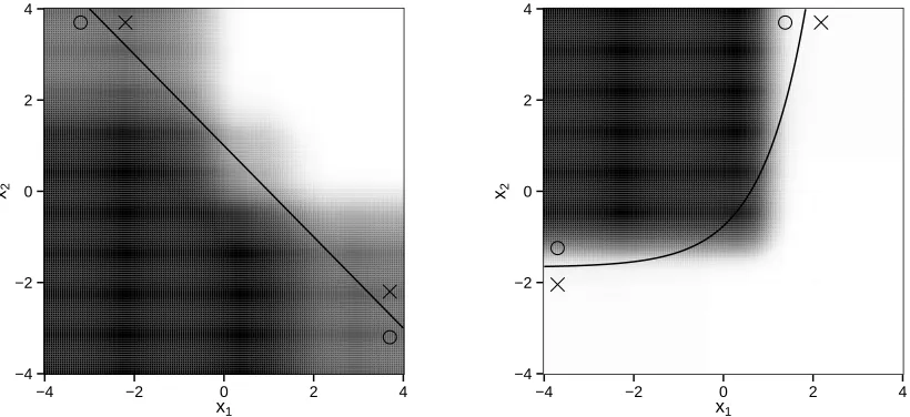
represen-tation of the decision list that requires only x1 in the first clause. Right: alternative representation of the same decision list that re-quires bothx1 and x2 in the first clause. . . 11 Figure 1.3 Left: average estimated regimes under setting II. Right: average

es-timated regimes under setting III. In both settings πopt cannot be represented as decision list. The solid line is the treatment decision boundary underπopt_{. The region where treatment 1 is better than} treatment 2 is marked by circles, while the region where treatment 2 is better than treatment 1 is marked by crosses. For every point (x1, x2)T, we compute the proportion of 1000 replications that the estimated regime recommends treatment 1 to a patient with covari-ate (x1, x2,0, . . . ,0) ∈ R10. The larger the proportion, the darker

the shade. . . 20 Figure 1.4 Top: estimated optimal treatment regime representable as a

deci-sion list. Bottom: treatment regime proposed by Gail and Simon (1985). . . 22 Figure 3.1 Estimated list-based DTR for the BMI dataset. . . 64 Figure A.1 Diagram and description of the decision list {_ea0}. . . 74 Figure A.2 Diagram and description of the decision list {(_ec1,ea1),ea

0

1}. . . 75 Figure A.3 Diagram and description of the decision list {(_ec0₁,_ea0₁),_ea1}. . . 75 Figure A.4 Diagram and description of the decision list {(_ec1,ea1),(ec2,ea2),ea

0 2}. It is possible that_ea2 =ea1 orea

0

2 =ea1. . . 76 Figure A.5 Diagram and description of the decision list {(_ec0₁,_ea0₁),(_ec2,ea2),ea

0 2}. It is possible that_ea2 =ea

0 1 orea

0 2 =ea

0

1. . . 78 Figure A.6 Diagram and description of the decision list{(_ec0₁,_ea0₁),(_ec2,ea2),(ec3,ea3),ea

0 3}. Some of the values of _ea0₁,_ea2,ea3,ea

0

3 can be equal. . . 79 Figure A.7 Diagram and description of the decision list{(_ec0₁,a_e0₁),(_ec0₂,_ea0₂),(_ec3,ea3),ea

0 3}. Some of the values of _ea0₁,_ea0₂,_ea3,ea

0

(12)

Chapter 1 Using Decision Lists to Construct

Interpretable and Parsimonious

Treatment Regimes

1.1 Introduction

(13)

regimes into clinical practice is, and should be, an incremental process wherein: (i) data are used to generate hypotheses about optimal treatment regimes; (ii) the generated hy-potheses are scrutinized by clinical collaborators for scientific validity; (iii) new data are collected for validation and new hypothesis generation, and so on. Within this process, it is crucial that estimated treatment regimes be interpretable to clinicians. Nevertheless, optimality, not interpretability, has been the focal point in the statistical literature on treatment regimes.

(14)

Classification-based estimators, also known as policy-search or value-search estima-tors, estimate the marginal mean of the outcome for every treatment regime within a pre-specified class and then take the maximizer as the estimated optimal regime. Ex-amples include marginal structural mean models (Robins et al., 2008; Orellana et al., 2010); robust marginal mean models (Zhang et al., 2012c); and outcome weighted learn-ing (Zhang et al., 2012a; Zhao et al., 2012, 2015b). Classification-based estimators of-ten rely on fewer assumptions about the conditional distribution of the outcome given treatment and patient information and thus may be more robust to model misspecifi-cation than regression-based estimators (Zhang et al., 2012c,a). Furthermore, because classification-based methods estimate an optimal regime within a pre-specified class, it is straightforward to impose structure on the estimated regime, e.g., interpretability, by restricting this class. We use robust marginal mean models with a highly interpretable yet flexible class of regimes to estimate a high-quality regime that can be immediately understood by clinical and intervention scientists.

(15)

presents with somatic anxiety score above 1 and retardation score above 2, the list rec-ommends nefazodone; otherwise, if the patient has Hamilton anxiety score above 23 and sleep disturbance score above 2, the list recommends psychotherapy; and otherwise the list recommends nefazodone + psychotherapy (combination). Thus, a treatment regime represented as a decision list can be conveyed as either a diagram or text and is eas-ily understood, in either form, by domain experts. Indeed, decision lists have frequently been used to display estimated treatment regimes (Shortreed et al., 2011; Moodie et al., 2012; Shortreed et al., 2014; Laber and Zhao, 2015) or to describe theory-based, i.e., not data-driven, treatment regimes (Shiffman, 1997; Marlowe et al., 2012).

Another important attribute of a decision list is that it “short circuits” measurement of patient covariates; e.g., in Figure 1.1, the Hamilton anxiety score and sleep disturbance score do not need to be collected for patients with somatic anxiety score above 1 and retardation score above 2. This is important in settings where patient covariates are expensive or burdensome to collect (e.g., Gail et al., 1999; Gail, 2009; Baker et al., 2009; Huang et al., 2015). We provide an estimator of the treatment regime that minimizes an expected cost among all regimes that optimize the marginal mean outcome.

1.2 Methodology

1.2.1 Framework

We assume that the observed data are {(Xi, Ai, Yi)}n_i₌₁, which comprise n independent

(16)

Start

somatic>1 and retardation>2

HAM−A>23 and sleep>2 FALSE

FALSE

TRUE

nefazodone

psychotherapy

combination

Figure 1.1 Estimated decision list for treating patients with chronic depression.

patient covariates;A ∈ A={1, . . . , m}is the treatment assigned; and Y ∈_Ris the out-come, coded so that higher values are better. A treatment regime, π, is a function from

Rp into A, so that under π a patient presenting with X =x is recommended treatment

π(x).

The value of a regime π is the expected outcome if all patients in the population of interest are assigned treatment according to π. To define the value, we use the set of potential outcomes {Y∗_(a)}

a∈A, where Y

∗_{(a) is the outcome that would be observed if a} subject were assigned treatment a. Define Y∗(π) = P

a∈AY

∗_(a)I_{{π(X) =}_a} _{to be the} potential outcome under regimeπ, andR(π) = E{Y∗_(π)}_{to be the value of regime}_{π. An} optimal regime, sayπopt, satisfiesR(πopt)≥R(π) for allπ. Let Π denote a class of regimes of interest. Classification-based estimation methods form an estimator ofR(π), sayR(π),b and then estimateπopt _using

b

(17)

algorithm for maximizingR(π) over Π. We discuss these topics in the next three sections.b

1.2.2 Estimation of

R

(

π

)

We make several standard assumptions: (A1) consistency: Y = Y∗(A); (A2) no unmea-sured confounders: {Y∗_(a)}

a∈A are conditionally independent of A given X; and (A3) positivity: there exists δ >0 so that Pr(A=a|X)≥δ for all a∈ A. Assumption (A2) is automatically satisfied in a randomized study but is untestable in observational studies (Robins et al., 2000). Under (A1)–(A3), it can be shown (Tsiatis, 2006) that

R(π) = E

m

X

a=1

I(A=a)

ω(X, a) {Y −µ(X, a)}+µ(X, a)

I{π(X) =a} !

, (1.1)

where ω(x, a) = Pr(A = a|X = x) and µ(x, a) = E(Y|X = x, A = a). Alternate expressions for R(π) exist (Zhang et al., 2012a); however, estimators based on (1.1) possess a number of desirable properties (see below).

To construct an estimator ofR(π) from (1.1) we replaceω(x, a) andµ(x, a) with esti-mated working models and replace the expectation with its sample analog. If treatment is randomly assigned independently of subject covariates, thenω(x, a) can be estimated by n−1Pn

i=1I(Ai = a). Otherwise, we posit a multinomial logistic regression model of

the formω(x, a) = exp (uT γa)

1 +Pm−1

j=1 exp (u T

γj) , a= 1, . . . , m−1, whereu=u(x)

is a known feature vector, andγ1, . . . , γm−1 are unknown parameters. Letω(x, a) denoteb the maximum likelihood estimator of ω(x, a), where γ1, . . . , γm−1 are replaced by maxi-mum likelihood estimators _bγ1, . . . ,bγm−1. We posit a generalized linear model for µ(x, a), g{µ(x, a)}=zT_β

(18)

constructed fromx, andβ1, . . . , βm are unknown parameters. We useµ(x, a) =b g −1_(zT

b βa)

as our estimator of µ(x, a), where βb₁, . . . ,βb_m are the maximum likelihood estimators of β1, . . . , βm.

Given estimators ω(x, a) and_b _bµ(x, a), an estimator of R(π) based on (1.1) is

b

R(π) = 1 n

n

X

i=1

m

X

a=1

I(Ai =a)

b

ω(Xi, a)

{Yi−µ(Xb i, a)}+µ(Xb i, a)

I{π(Xi) =a}. (1.2)

For any fixedπ,R(π) is doubly robust in the sense that it is a consistent estimator ofb R(π) if either the model forω(x, a) orµ(x, a) is correctly specified (Tsiatis, 2006; Zhang et al., 2012c). As a direct consequence, R(π) is guaranteed to be consistent in a randomizedb study, asω(x, a) is known by design. Furthermore, if both models are correctly specified, thenR(π) is semiparametric efficient; i.e., it has the smallest asymptotic variance amongb the class of regular, asymptotically linear estimators (Tsiatis, 2006).

1.2.3 Regimes Representable as Decision Lists

Gail and Simon (1985) present an early example of a treatment regime using data from the NSABP clinical trial. The treatment regime they propose is

If age≤50 and PR≤10 then chemotherapy alone;

else chemotherapy with tamoxifen,

(19)

Formally, a treatment regime, π, that is representable as a decision list of length Lis described by{(c1, a1), . . . ,(cL, aL), a0}, wherecj is a logical condition that is true or false

for eachx∈_Rp_{, and}_a

j ∈ Ais a recommended treatment,j = 0, . . . , L. As a special case,

L= 0 is allowed. The corresponding treatment regime {a0} gives the same treatment a0 to every patient. Hereafter, let Π denote the set of regimes that are representable as a decision list. Clearly, the regime proposed by Gail and Simon (1985) is a member of Π.

DefineT(cj) ={x∈Rp : cjis true forx},j = 1, . . . , L;R1 =T(c1),Rj ={∩`<jT(c`)c}T

T(cj), j = 2, . . . , L; and R0 = TL

`=1T(c`)

c_{, where} _Sc _{is the complement of the set} _S.

Then a regime π ∈Π can be written as π(x) = PL

`=0a`I(x∈ R`), which has structure

If c1 then a1;

else if c2 then a2;

... (1.3)

else if cL then aL; else a0.

(20)

parsimony and interpretability, we restrictcj so that T(cj) is one of the following sets:

[1]: {x∈_Rp _: _x

j1 ≤τ1}, [6]: {x∈R

p _: _x

j1 ≤τ1 orxj2 ≤τ2}, [2]: {x∈_Rp : xj1 ≤τ1 and xj2 ≤τ2}, [7]: {x∈R

p

: xj1 ≤τ1 orxj2 > τ2}, [3]: {x∈_Rp _: _x

j1 ≤τ1 and xj2 > τ2}, [8]: {x∈R

p _: _x

j1 > τ1 or xj2 ≤τ2}, [4]: {x∈_Rp _: _x

j1 > τ1 and xj2 ≤τ2}, [9]: {x∈R

p _: _x

j1 > τ1 or xj2 > τ2}, [5]: {x∈_Rp _: _x

j1 > τ1 and xj2 > τ2}, [10]: {x∈R

p _: _x

j1 > τ1},

(1.4)

where j1 < j2 ∈ {1, . . . , p} are indices and τ1, τ2 ∈ R are thresholds. We believe that the conditions that dictate the sets in (1.4), e.g., xj1 ≤ τ1 and xj2 ≤ τ2, are more easily interpreted than those dictated by linear thresholds, e.g., α1xj1 +α2xj2 ≤ α3, as the former are more commonly seen in clinical practice.

(21)

Uniqueness and Minimal Cost of a Decision List

For a decision list π described by {(c1, a1), . . . ,(cL, aL), a0}, let N` denote the cost of

measuring the covariates required to check logical conditions c1, . . . , c`. Hereafter, for

simplicity, we assume that this cost is equal to the number of covariates needed to check c1, . . . , c`, but it can be extended easily to a more complex cost function

re-flecting risk, burden, and availability. The expected cost of applying treatment rule π(x) = PL

`=0a`I(x∈ R`) is N(π) =

PL

`=1N`Pr (X ∈ R`) + NLPr (X ∈ R0), which is smaller than NL = NL

PL

`=0Pr(X ∈ R`), the cost of measuring all covariates in the

treatment regime. This observation reflects the benefit of the short-circuit property. A decision list π described by {(c1, a1), . . . ,(cL, aL), a0} need not be unique in that there may exist an alternative decision list π0 described by {(c0

1, a 0

1), . . . ,(c 0

L0, a0_L0), a0₀}

such that π(x) = π0(x) for all x but L6= L0, or L = L0 but cj 6= c0j or aj 6=a0j for some

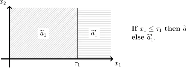
j ∈ {1, . . . , L}. This is potentially important because the expected costsN(π) and N(π0) might differ substantially. Figure 1.2 shows two representations, π and π0, of the same decision list both withL=L0 = 2 but with different clauses. The cost of the decision list in the middle panel, π, is N(π) = N1Pr(X1 > τ1) +N2Pr(X1 ≤ τ1), whereas the cost of the decision list in the right panel, π0, is N(π0) = N2 ≥ N(π) with strict inequality if N2 > N1 and Pr(X1 > τ1) > 0. Thus, π is preferred to π0 in settings where X2 is a biomarker that is expensive, burdenome, or potentially harmful to collect (e.g., Huang et al., 2015, and references therein).

Therefore, among all decision lists achieving the value R(πopt_{), where} _πopt _{is an} op-timal regime as defined previously, we seek to estimate the one that minimizes the cost. Defining Lr to be the level set

(22)

a1 a2

a0 τ2

τ1 x2

x1

Decision listπ:

If x1 > τ1 then a1;

else if x2 > τ2 then a2;

else a0.

Decision listπ0:

If x1 ≤τ1 and x2 > τ2 then a2;

else if x1 > τ1 then a1;

else a0.

Figure 1.2 Left: diagram of a decision list dictated by regionsR1 =

x∈_R2 _: _x

1 > τ1 ,

R₂ =

x∈_R2 _:_x

1 ≤τ1, x2> τ2 , andR0 =

x∈_R2 _: _x

1 ≤τ1, x2 ≤τ2 , and treatment recommendationsa1,a2, anda0. Middle: representation of the decision list that requires only x1 in the first clause. Right: alternative representation of the same decision list that requires both x1 andx2 in the first clause.

regime in the set arg minπ∈L{R(πopt_)}N(π). Define L(r) =b

π ∈Π : R(π) =b r . Let π_e be an estimator of an element in the set arg maxπ∈ΠR(π). In the following we provide anb algorithm that ensures our estimator,_bπ, belongs to the set arg min_π_∈

b

L{Rb(_eπ)}Nb(π), where b

N(π) is defined by replacing the probabilities in N(π) with sample proportions.

1.2.4 Computation

Estimation proceeds in two steps: (i) approximate an element _eπ ∈ arg maxπ∈ΠR(π),b whereR(π) is constructed using (1.2); and (ii) find an elementb

b

π∈arg min_π_∈ b

L{Rb(_eπ)}Nb(π).

Approximation of arg maxπ∈ΠR(π)b

(23)

val-ues Xj. These cutoffs might be dictated by clinical guidelines, e.g., if the covariate is a

comorbid condition then the thresholds might reflect low, moderate, and high levels of impairment; alternatively, these cutoffs could be chosen to equal empirical or theoreti-cal percentiles of that covariate. There is no restriction imposed on these cutoffs. Let C denote the set of all conditions that induce regions of the form in (1.4) with the cutoffs τjk ∈ Xjk for k= 1,2,jk ∈ {1, . . . , p}.

Before giving the details of the algorithm, we provide a conceptual overview. The algorithm first uses exhaustive search to find a decision list with exactly one clause, of the form π ={(c1, a1), a01}, which maximizesR(π). Letb {(

e

c1,ea1),ea 0

1}denote this decision list. The algorithm then uses exhaustive search to find the decision list that maximizes

b

R(π) over decision lists with exactly two clauses, the first of which must be either (_ec1,ea1) or (_ec0₁,_ea0₁), where _ec0₁ is the negation of c1_e such that T(_ec0₁) = T(_ec1)c; e.g., if _ec1 has the formxj1 ≤τ1 and xj2 ≤τ2, thenec

0

1 would be xj1 > τ1 or xj2 > τ2. Although the decision lists {(_ec1,ea1),ea

0

1} and {(ec 0 1,ea

0

1),ea1} yield identical treatment recommendations and have the same value, their first clauses are distinct, and may lead to substantially different final decision lists. Hence it is necessary to consider both possibilities for the first clause. The algorithm proceeds recursively by adding one clause at a time until some stopping criterion (described below) is met.

Hereafter, for a decision list π described by{(c1, a1), . . . ,(cL, aL), a0}for someL≥0,

write b

R[{(c1, a1), . . . ,(cL, aL), a0}] to denote R(π); e.g., forb L = 0, Rb[{a0}] is the estimated value of the regime that assigns treatment a0 to all patients. For any decision list with a vacuous condition, e.g.,{∩`<jT(c`)c}

T

(24)

−∞. Letzρbe the 100ρ percentile of the standard normal distribution. Let Πtemp denote the set of regimes to which additional clauses can be added, and let Πfinal denote the set of regimes that have met one of the stopping criteria. The algorithm is as follows, and an illustrative example with a step-by-step run of the algorithm is given in the Appendix.

Step 1. Choose a maximum list length Lmax and a critical level α ∈ (0,1). Compute e

a0 = arg maxa0∈ARb[{a₀}]. Set Π_temp =∅ and Π_final =∅.

Step 2. Compute (_ec1,_ea1,_ea₁0) = arg max₍_c₁_,a₁_,a0

1)∈C×A×ARb[{(c1, a1), a 0

1}] and ∆1b = b

R[{(_ec1,_ea1),_ea0₁}]−Rb[{_ea0}]. If∆1b < z1−α

d Var ∆1b

1/2

then letπ ={_ea0}, set Πfinal ={π}, and go to Step 5; otherwise let π ={(_ec1,ea1),ea

0 1}, π

0 ₌_{( e

c0₁,_ea0₁),_ea1}, set Πtemp ={π, π0}, and proceed to Step 3, where_ec0₁ is the negation of _ec1.

Step 3.Pick an elementπ ∈Πtemp, sayπ =

(c1, a1), . . . ,(cj−1, aj−1), a0_j−1 , wherej−1 is the length ofπ. Removeπfrom Πtemp. With the clauses (c1, a1), . . . ,(cj−1, aj−1) held fixed, compute (_ecj,eaj,ea

0

j) = arg max(cj,aj,a0

j)∈C×A×ARb

(c1, a1), . . . ,(cj−1, aj−1),(cj, aj), a0j and

b ∆j = Rb

(c1, a1), . . . ,(cj−1, aj−1),(ecj,eaj),ea 0

j −Rb

(c1, a1), . . . ,(cj−1, aj−1), a0j−1 . If b

∆j < z1−α

d Var ∆bj

1/2

, then let π =

(c1, a1), . . . ,(cj−1, aj−1), a0j−1 , and set Πfinal = ΠfinalS{π}; otherwise if j =Lmax, let π =

(c1, a1), . . . ,(cj−1, aj−1),(ecj,eaj),ea 0

j , and set

Πfinal = ΠfinalS{π}; otherwise set Πtemp = ΠtempS{π, π0}, where ec 0

j is the negation of ecj, π =(c1, a1), . . . ,(cj−1, aj−1),(_ecj,eaj),ea

0

j , andπ

0 ₌

(c1, a1), . . . ,(cj−1, aj−1),(_ec0_j,_ea0_j),_eaj .

Step 4. Repeat Step 3 until Πtemp becomes empty.

(25)

The above description is simplified to illustrate the main ideas. The actual implemen-tation of this algorithm avoids exhaustive searches by pruning the search spaceC ×A×A. It also avoids explicit construction of Πtemp and Πfinal. Complete implementation details are provided in the Appendix. In the algorithm, the decision list stops growing if either the estimated increment in the value,∆bj, is not sufficiently large compared to an estimate

of its variation, d Var ∆bj

1/2

, or if it reaches the pre-specified maximal lengthLmax. We estimate Var(∆b_j) using large sample theory; the expression is given in the Appendix. This variance estimator is a crude approximation, as it ignores uncertainty introduced by the estimation of the decision lists; however, it can be computed quickly, and in simulated experiments it appears sufficient for use in a stopping criterion. The significance level α is a user-chosen tuning parameter. In our simulation experiments, we chose α = 0.05; results were not sensitive to this choice (see Appendix). To avoid lengthy lists, we set Lmax = 10. Nevertheless, in our simulations and applications the estimated lists never reach this limit. Finally, it may be desirable in practice to restrict the set of candidate clauses so that, for each j, the number of subjects inRb_j ={∩_`<jT(

b c`)c}

T

T(_bcj) exceeds

some minimal threshold. This can be readily incorporated into the above algorithm by simply discarding candidate clauses that induce partitions that contain an insufficient number of observations.

The time complexity of the proposed algorithm is O2Lmax_mp2_n_{+ (max}

j#Xj)2

(see Appendix), where #Xj is the number of cutoff values inXj. Because 2Lmax andm are

constants that are typically small relative top2

n+ (maxj#Xj)2 , the time complexity

is essentiallyO(np2_{) provided that max}

j#Xj is either fixed or diverges more slowly than

(26)

the proposed algorithm runs very fast and scales well in both dimension p and sample size n.

Finding an Element of arg min_π_∈ b

L{Rb(_eπ)}Nb(π) To find an element within the set arg min_π_∈

b

L{Rb(_eπ)}Nb(π), we enumerate all regimes in L

b

R(_eπ) with length no larger than Lmax and select among them the list with the minimal cost. The enumeration algorithm is recursive and requires a substantial amount of bookkeeping; therefore, we describe the basic idea here and defer implementation details to the Appendix. Suppose _eπ is described by {(_ec1,ea1), . . . ,(ecL,eaL),ea0}. Call a condition of the form xj ≤ τj an atom. There exist K ≤ 2L atoms, say d1, . . . , dK,

such that each clause _ec`, ` = 1, . . . , L, can be expressed using the union, intersection,

and/or negation of at most two of these atoms. The algorithm proceeds by generating all lists with clauses representable using the foregoing combinations of at most two atoms. To reduce computation time, we use a branch-and-bound scheme (Brusco and Stahl, 2006) that avoids constructing lists with vacuous conditions or those that are provably worse than an upper bound on min_π_∈

b

L{Rb(_eπ)}N(π). In the simulation experiments in the next section, the average runtime for the enumeration algorithm was less than one second running on a single core of a 2.3GHz AMD Opteron™processor and 1GB of DDR3 RAM.

1.3 Simulation Experiments

(27)

and continuous outcomes; (ii) binary and trinary treatments; (iii) correctly and incor-rectly specified models; and (iv) low- and high-dimensional covariates. The class of data-generating models that we consider is as follows. Covariates are drawn from a p-dimensional Gaussian distribution with mean zero and autoregressive covariance matrix such that cov(Xk, X`) = 4(1/5)|k−`|, and the treatments are sampled uniformly so that

P(A=a|X =x) = 1/m for allx ∈_Rp _and _a_{∈ A. Let}_{φ(x, a) be a real-valued function}

of x and a; given X =x and A=a, continuous outcomes are normally distributed with mean 2 +x1 +x3 +x5 +x7 +φ(x, a) and variance 1, whereas binary outcomes follows a Bernoulli distribution with success probability expit{2 +x1+x3+x5+x7+φ(x, a)}, where expit(u) = exp(u)/{1 + exp(u)}. Table 1.1 lists the expressions of φ used in our generative models and the number of treatments,m, inA. Under these outcome models, the optimal regime is πopt(x) = arg maxaφ(x, a).

For comparison, we estimateπopt_{by parametric}_{Q-learning, nonparametric}_Q-learning, outcome weighted learning (OWL, Zhao et al., 2012) and modified covariate approach (MCA, Tian et al., 2014). For parametric Q-learning, we use linear regression when Y is continuous and logistic regression when Y is binary. The linear component in the re-gression model has the form Pm

a=1I(A = a)(1, X T_)β

a, where β1, . . . , βm are unknown

(28)

Gaus-sian kernels are used and we follow the same tuning strategy as in Zhao et al. (2012). For MCA, we incorporate the efficiency augmentation term described in Tian et al. (2014). Both OWL and MCA are limited to two treatment options.

To implement our method, the mean model,µ(x, a), in (1.1), is estimated as in para-metric Q-learning. The propensity scoreω(x, a) is estimated by n−1Pn

i=1I(Ai =a). All the comparison methods result in treatment regimes that are more difficult to interpret than a decision list; thus, our intent is to show that decision lists are competitive in terms of the achieved value of the estimated regime, _E{R(_bπ)}, while being significantly more interpretable and less costly.

(29)

Table 1.1 The second column gives the number of treatment optionsm. The third column gives the set ofφ functions used in the outcome models. The fourth column specifies the form of the optimal regime πopt(x) = arg maxaφ(x, a) where: “linear” indicates thatπopt(x) =

arg maxa{(1, xT)βa}for some coefficient vectorsβa ∈ Rp+1,a ∈ A; “decision list” indicates thatπopt is representable as a decision list; and “nonlinear” indicates thatπopt(x) is neither linear nor representable as a decision list.

Setting m Expression ofφ Form of πopt

I 2 φ1(x, a) =I(a = 2){3I(x1 ≤1, x2 >−0.6)−1} decision list II 2 φ2(x, a) =I(a = 2)(x1+x2−1) linear III 2 φ3(x, a) =I(a = 2) arctan(exp(1+x1)−3x2−5) nonlinear IV 2 φ4(x, a) =I(a = 2)(x1−x2+x3−x4) linear

V 3 φ5(x, a) =I(a = 2){4I(x1 >1)−2}

+I(a= 3)I(x1 ≤1){2I(x2 ≤ −0.3)−1}

decision list VI 3 φ6(x, a) =I(a = 2)(2x1) +I(a= 3)(−x1x2) nonlinear VII 3 φ7(x, a) =I(a = 2)(x1−x2) +I(a= 3)(x3−x4) linear

estimator. Nonparametric Q-learning OWL always use all covariates, so their costs are always equal to p.

In the Appendix, we derive point estimates and prediction intervals for R(_bπ). We also present simulation results to illustrate the accuracy of variable selection for the decision list.

1.4 Applications

1.4.1 Breast Cancer Data

(30)

Table 1.2 The average value and the average cost of estimated regimes in simulated exper-iments. In the header, p is the dimension of patient covariates; DL refers to the proposed method using decision list;Q1 refers to parametricQ-learning;Q2 refers to nonparamet-ric Q-learning; OWL1 and OWL2 refer to outcome weighted learning with linear kernel and Gaussian kernel, respectively; MCA refers to modified covariate approach with efficiency aug-mentation. OWL and MCA are not applicable under Setting V, VI and VII.

p Setting Value Cost

DL Q1 Q2 OWL1 OWL2 MCA DL Q1 MCA

Continuous response

10

I 2.78 2.53 2.53 2.33 2.29 2.54 1.64 9.0 5.1

II 2.70 2.80 2.79 2.61 2.54 2.80 1.64 9.0 5.1

III 2.59 2.54 2.53 2.29 2.24 2.55 1.68 9.1 4.9

IV 2.89 3.37 3.35 3.16 3.09 3.37 2.50 9.5 7.4

V 2.90 2.67 2.59 − − − 1.90 9.5 −

VI 3.98 3.46 3.95 − − − 1.61 9.2 −

VII 3.22 3.75 3.73 − − − 2.56 9.7 −

50

I 2.76 2.51 2.36 2.21 2.19 2.53 1.80 21.3 9.2

II 2.70 2.79 2.73 2.26 2.27 2.79 1.64 21.4 9.3

III 2.59 2.52 2.35 2.16 2.12 2.54 1.71 23.1 9.0

IV 2.89 3.36 3.27 2.76 2.70 3.36 2.53 25.4 14.9

V 2.87 2.63 2.33 − − − 2.14 28.5 −

VI 3.95 3.43 3.47 − − − 1.69 26.6 −

VII 3.21 3.74 3.61 − − − 2.55 30.8 −

Binary response

10

I 0.77 0.74 0.69 0.73 0.73 0.74 1.94 8.9 4.1

II 0.71 0.72 0.60 0.71 0.71 0.72 1.69 9.2 5.3

III 0.73 0.73 0.68 0.72 0.72 0.73 2.10 9.2 4.7

IV 0.71 0.76 0.66 0.75 0.74 0.75 2.40 9.6 8.4

V 0.75 0.73 0.62 − − − 2.52 9.6 −

VI 0.79 0.75 0.64 − − − 2.09 9.5 −

VII 0.77 0.81 0.69 − − − 2.83 9.9 −

50

I 0.76 0.73 0.69 0.71 0.70 0.73 2.64 21.9 8.3

II 0.71 0.72 0.60 0.70 0.69 0.71 1.87 26.2 6.4

III 0.73 0.72 0.67 0.70 0.69 0.72 2.53 25.0 7.3

(31)

● ●

−4 −2 0 2 4

x1

x2

●

−4 −2 0 2 4

x1

x2

(32)

plus tamoxifen to all others. Because the variables involved in the treatment regime con-structed by Gail and Simon were chosen using clinical judgment, it is of interest to see what regime emerges from a more data-driven procedure. Thus, we use the proposed method to estimate an optimal treatment regime in the form of a decision list using data from the NSABP trial.

As in Gail and Simon (1985), we take three-year disease-free survival as the outcome, so that Y = 1 if the subject survived disease-free for three years after treatment, and Y = 0 otherwise. Patient covariates are age (years), PR (fmol), estrogen receptor level (ER, fmol), tumor size (centimeters), and number of histologically positive nodes (number of nodes, integer). We estimated the optimal treatment regime representable as a decision list using data from the 1164 subjects with complete observations on these variables. Because treatment assignment was randomized in NSABP, we estimated ω(x, a) by the sample proportion of subjects receiving treatment a. Based on exploratory analyses, we estimated µ(x, a) using a logistic regression model with transformed predictors z = z(x) ={age,log(1 + PR),log(1 + ER),tumor-size,log(1 + number-of-nodes)}T_.

The estimated optimal treatment regime representable as a decision list is given in the top panel of Figure 1.4; the regime estimated by Gail and Simon is given in the bottom panel of this figure. The structure of the two treatment regimes is markedly similar. The treatment recommendations from the two regimes agree for 92% of the patients in the NSABP data. In this data set, 33% of the patients have a PR value less than 3; 13% of the patients have a PR values between 3 and 10; and 54% of the patients have a PR value greater than 10.

(33)

Start

age≤51 and PR≤3

FALSE

TRUE

chemotherapy alone

chemotherapy with tamoxifen

Start

age≤50 and PR≤10

FALSE

TRUE

chemotherapy alone

chemotherapy with tamoxifen

(34)

patients with age+7.98 log(1+PR)≤60 receive chemotherapy alone and all others receive chemotherapy plus tamoxifen. However, this regime was built using only age and PR as potential predictors with no data-driven variable selection. In contrast, the proposed method selects age and PR from the list of potential predictors. For completeness, we also implemented parametricQ-learning using a logistic regression model with covariate vector z. The estimated regime recommends chemotherapy alone if 1.674−0.021 age− 0.076 log(1+PR)−0.116 log(1+ER)−0.024 tumor-size−0.274 log(1+number-of-nodes)≥ 0 and chemotherapy with tamoxifen otherwise. The treatment recommendation dictated by parametricQ-learning agrees with that dictated by decision list for 86% of the subjects in the data set.

To estimate the survival probability under each estimated regime, we use cross-validation. The data set was randomly divided into a training set containing 80% of the subjects and a test set containing 20% of the subjects. The optimal regime was esti-mated using both approaches on the training set, and its value was computed using (1.2) (with µ_b≡0) on the test set. To reduce variability, this process was repeated 100 times. The estimated survival probability is 0.65 for the regime representable as decision list and 0.66 for the regime obtained from parametricQ-learning. Thus, the proposed method greatly improves interpretability while preserving quality.

1.4.2 Chronic Depression Data

(35)

shown to be the most beneficial in terms of efficacy as measured by the Hamilton Rating Scale for Depression score (HRSD). However, the combination treatment is significantly more expensive and burdensome than monotherapy. Therefore, it is of interest to con-struct a treatment regime that recommends combination therapy only to subjects for whom there is a significant benefit over monotherapy.

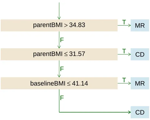
Because lower HRSD indicates less severe symptoms, we define outcomeY =−HRSD to be consistent with our paradigm of maximizing the mean outcome. Patient covariates comprise 50 pretreatment variables, including personal habits and difficulties, medica-tion history and various scores from several psychological quesmedica-tionnaires; a list of these variables is given in the Appendix. We estimate an optimal regime using data from the n = 647 (of 680 enrolled) subjects in the clinical trial with complete data. Because treatments were randomly assigned, we estimated ω(x, a) by the sample proportion of subjects receiving treatment a. We estimated µ(x, a) using a penalized linear regression model with all patient covariates and treatment by covariate interactions. Penalization was implemented with a LASSO penalty tuned using 10-fold cross-validated prediction error.

(36)

disturbance to psychotherapy alone. All others are assigned to the combination therapy. The estimated regime contains only four covariates. In contrast, the regime estimated by parametric Q-learning using linear regression and LASSO penalty involves a linear combination of twenty-four covariates, making it difficult to explain and expensive to implement. To compare the quality of these two regimes, we use random-split cross-validation as in Section 4.1. The estimated HRSD score under the regime representable as decision list is 12.9, while that under the regime estimated by parametric Q-learning is 11.8. Therefore, by using decision lists we are able to obtain a remarkably more parsi-monious regime with high quality, which facilitates easier interpretation.

1.5 Discussion

Data-driven treatment regimes have the potential to improve patient outcomes and gen-erate new clinical hypotheses. Estimation of an optimal treatment regime is typically conducted as a secondary, exploratory analysis aimed at building knowledge and inform-ing future clinical research. Thus, it is important that methodological developments are designed to fit this exploratory role. Decision lists are a simple yet powerful tool for estimation of interpretable treatment regimes from observational or experimental data. Because decision lists can be immediately interpreted, clinical scientists can focus on the scientific validity of the estimated treatment regime. This allows the communications between the statistician and clinical collaborators to focus on the science rather than the technical details of a statistical model.

(37)

(38)

Chapter 2 Interpretable Dynamic Treatment

Regimes

2.1 Introduction

(39)

even under the simplest generative models the optimal regime is a nonlinear function of patient information (Robins, 2004; Schulte et al., 2014; Laber et al., 2014); consequently, to avoid model misspecification, a recent trend is to apply flexible supervised learning methods to estimate optimal treatment regimes. These flexible methods include direct-search using large-margin classifiers (Zhao et al., 2012, 2015b; Kang et al., 2014; Zhao et al., 2015a; Xu et al., 2015b); Q-learning with non-parametric regression models (Qian and Murphy, 2011; Zhao et al., 2011; Moodie et al., 2013; Zhou and Kosorok, 2016); and tree-based methods (Zhang et al., 2012b; Laber and Zhao, 2015; Zhang et al., 2015; Doove et al., 2015). Further testament to the popularity of these methods is that the Journal of the American Statistical Association’s Theory and Methods Invited Paper and the Case Studies and Applications Invited Paper at the 2016 Joint Statistical Meetings will feature non-parametric methods for estimating treatment regimes (Zhou et al., 2015; Xu et al., 2015a).

(40)

each of which is represented as a sequence if-then statements mapping logical clauses to treatment recommendations. Decision rules of this form are a special case of tree-based rules, known as decision lists (Rivest, 1987; Marchand and Sokolova, 2005; Letham et al., 2012; Wang and Rudin, 2015; Zhang et al., 2015), that are immediately interpretable in a domain context as they can be expressed in either flow-chart or paragraph form. Thus, regimes of this form are amenable to critique and examination by clinicians and facilitate collaborative, iterative development of data-driven precision medicine. Furthermore, we shall show that despite the structure imposed by the decision lists, they are sufficiently expressive so as to provide high-quality regimes even under non-linear generative mod-els previously used in the literature to illustrate the value of non-parametric estimation methods.

(41)

results on convergence rates for decision lists and are therefore of independent interest. A third contribution is the proposed estimation algorithm used to construct the decision lists at each stage. This algorithm reduces computation time of naive recursive-splitting algorithm from O(n3) to O(nlog n) where n is the number of subjects in the sample, furthermore we modify the splitting criteria proposed by Zhang et al. (2015) to avoid (asymptotically) becoming stuck in a local mode.

In Section 2.2, we describe list-based treatment regimes and describe our estimation algorithm. In Section 2.3, we prove consistency of the proposed estimator and derive rates of convergence. In Section 2.4, we demonstrate the finite sample performance of the proposed method using simulation experiments. We illustrate the proposed method using data from a clinical trail in Section 2.5 and make concluding remarks in Section 2.6.

2.2 Methodology

2.2.1 Framework

Consider n i.i.d.observations collected from a sequential clinical trial with T stages; the proposed methodology also applies to observational data provided that standard causal assumptions required forQ-learning are satisfied (see Schulte et al., 2014, for a statement of these assumptions). In the assumed setup the observed data are {(Sit, Ait, Yit) : t =

1, . . . , T}n

i=1, which comprise i.i.d. trajectories of the form {(St, At, Yt) : t = 1, . . . , T}

where: St ∈ Rpt is a vector of covariates measured at the beginning of the t-th stage;

At ∈ At is the treatment actually received during the t-th stage; and Yt ∈ R is a scalar

(42)

available treatment options at the t-th stage. The final outcome of interest is the sum of immediate outcomes, Y = PT

t=1Yt. We assume that larger values of Y are better. Let

Xt denote the information available to the decision maker at stage t so that X1 = S1 and Xt = (XtT−1, At−1, Yt−1,StT)

T

for t > 1. Let Xt ⊂ Rdt be the support of Xt, where

dt=Pt_s₌₁ps+ 2(t−1) is the dimension ofXt.

A treatment regime π = (π1, . . . , πT) is a sequence of functions πt : Xt → At so

that under π a patient presenting with Xt = xt at stage t is recommended treatment

πt(xt). For any regime π, letEπ denote expectation with respect to distribution induced

by assigning treatments according to π. Given a class of regimes Π, an optimal regime satisfies,πopt _∈_{Π and}

Eπ

opt

Y ≥_Eπ_Y _{for all}_π _∈_{Π. Our goal is to construct an estimator}

of πopt when Π is the class of list-based regimes. Each decision rule πt in a list-based

regime has the form:

If xt∈Rt1 then at1; else if xt ∈Rt2 then at2; ...

else if xt ∈RtLt then atLt, (2.1)

where: each Rt` is a subset of Xt with the restriction that RtLt = Xt; at` ∈ At; ` =

1, . . . , Lt; andLtis the length ofπt. Thus, a compact representation ofπtis{(Rt`, at`)}Lt_`₌₁.

(43)

two covariates, hence Rt` is an element of

Rt={Xt, {x∈ Xt:xj1 ≤τ1}, {x∈ Xt:xj1 > τ1},

{x∈ Xt:xj1 ≤τ1 and xj2 ≤τ2}, {x∈ Xt :xj1 ≤τ1 and xj2 > τ2}, {x∈ Xt:xj1 > τ1 and xj2 ≤τ2}, {x∈ Xt :xj1 > τ1 and xj2 > τ2}:

1≤j1 < j2 ≤dt, τ1, τ2 ∈R}, (2.2)

where j1, j2 are indices and τ1, τ2 are thresholds. We also impose an upper bound, Lmax, on list length Lt for all t. Hence, the class of regimes of interest is Π = ⊗Tt=1Πt, where

Πt={{Rt`, at`}Lt`=1 :Rt`∈ Rt, at`∈ At, Lt≤Lmax}.

Remark 1. We omit sets of the form{xt ∈ Xt :xj1 ≤τ1 orxj2 ≤τ2} in the definition of Rt because such sets are expressible in terms of the sets already inRt. For example, the

clause “ifxt ∈Rt1 then at1” withRt1 ={xt∈ Xt:xtj1 ≤τ1 or xtj2 ≤τ2} can be written as “if xt ∈ R0t1 then at1; else if xt ∈ R0t2 then at1” with R0t1 = {xt ∈ Xt : xtj1 ≤ τ1} and R_t0₂ = {xt ∈ Xt : xtj2 ≤ τ2}. Moreover, the latter form has the benefit of avoiding the measurement of xj2 for subjects satisfying xj1 ≤ τ1, which may be an important consideration if xj2 refers to some biomarker that is expensive to measure (see Zhang et al., 2015, for discussion of decision lists and measurement cost).

Remark 2. Under certain generative models, distinct sets in Rt may correspond to the

(44)

ensure that different sets in Rt correspond to different groups of subjects. To see this,

suppose (Xt1, Xt2)T can take three possible values: (0,0)T, (1,0)T and (1,1)T, e.g., if Xt1 and Xt2 are indicators of two symptoms where the second symptom can be present only when the first symptom is present. In this case, the set {x ∈ Xt : x1 ≤ 0} and the set {x ∈ Xt : x1 ≤ 0 and x2 ≤ 0} correspond to the same group of subjects. Therefore,

we allow the thresholds to take arbitrary values. In our theoretical analysis, we quantify dissimilarity of sets in Rt using a distance that accounts for the distribution ofXt.

To estimateπoptwe combine non-parametricQ-learning with policy-search (see Taylor et al., 2015, for a discussion of this idea in the context of single decision point). To develop our ideas, we first provide a high-level schematic for our algorithm, then we describe implementation and modeling details, and finally we discuss a computational insight that improves computation time.

Define QT(xT, aT) = E(YT|XT = xT, AT = aT) then it can be shown that πTopt =

arg maxπ∈ΠTEQT {XT, π(XT)}. Recursively, for t = T − 1, . . . ,1 define Qt(xt, at) =

EYt+Qt+1

Xt+1, πtopt+1(Xt+1)

Xt=xt, At=at

and subsequently it can be shown that πopt_t = arg maxπt∈ΠtEQt{Xt, πt(Xt)} (Schulte et al., 2014). For each t = 1, . . . , T

let Qt denote a postulated class of models for Qt. Q-learning with policy-search follows

directly from the foregoing definitions; a schematic is as follows.

(S1) Construct an estimator of QT in QT, e.g., one could use penalized least squares

b

QT = arg minQT∈QT

Pn

i=1{YiT −QT(XiT, AiT)} 2

+PT(QT), where PT(QT) is a

penalty on the complexity ofQT. DefinebπT = arg maxπ∈ΠT

Pn

(45)

(S2) Recursively, for t=T −1, . . . ,1 construct an estimator of Qt inQt, say Qb_t, e.g.,

b

Qt= arg min Qt∈Qt

n

X

i=1 n

Yit+Qbt+1

Xi(t+1),bπt+1(Xi(t+1)) −Qt(Xit, Ait) o2

+Pt(Qt),

where Pt(Qt) is a penalty on the complexity ofQt. Define bπt= arg maxπt∈Πt

Pn

i=1Qb_t{X_it, π_t(X_it)}.

Implementation of the preceding schematic requires a choice of models for the Q-functions, a means of constructing an estimator within this class, and an algorithm for computing arg maxπt∈Πt

Pn

i=1Qb_t{X_it, π_t(X_it)}. In our implementation, we use kernel ridge regression with an extended Gaussian kernel to construct estimators of the Q-functions and a greedy stepwise algorithm to approximate π_bt from the estimated

Q-functions.

2.2.2 Kernel Ridge Regression

We use kernel ridge regression to estimate the Q-functions. Starting with the last stage, letKT(·,·) be a symmetric and positive definite function fromRdT×RdT toR, and letHT

be the corresponding reproducing kernel Hilbert space (RKHS). In our implementation, we employ an extension of the Gaussian kernel that uses different scaling factors in different variables:KT(x,z) = exp

n −PdT

j=1γT j(xj−zj)2

o

, whereγT = (γT1, . . . , γT dT)T

is a tuning parameter and γT j > 0 for all j. For each a ∈ AT, we estimate QT(·, a) via

penalized least squares

b

QT(·, a) = arg min f∈_HT

n−1 X

i∈IT a

(46)

where IT a ={i :AiT =a}, and λT >0 is a tuning parameter. LetYT a= (YiT)i∈IT a and

KT a ={K(XiT,XjT)}i,j∈IT a. By the representer theorem (Kimeldorf and Wahba, 1971),

b

QT(x, a) =

P

i∈IT aKT(x,XiT)βbiT a, whereβbT a = (βbiT a)i∈IT asatisfyβbT a= arg minβkYT a−

KT aβk2 +nλTβTKT aβ. Define πbT = arg maxπT∈ΠT

Pn

i=1Qb_T {X_{T i}, π_T(X_{T i})}.

Similarly, for each t < T let _Ht be the RKHS induced by the kernel Kt(x,z) =

expn−Pdt

j=1γtj(xj−zj)

2o_{, and}_γ

t= (γt1, . . . , γtdt)T is a tuning parameter. Recursively,

for each t < T, at∈ At, estimate Qt(·, a) by

b

Qt(·, a) = arg min f∈_Ht

n−1 X

i∈Ita

h

Yit+Qb_t₊₁{X_i,t₊₁, b

πt+1(Xi,t+1)} −f(Xit)

i2

+λtkfk2_Ht,

where Ita ={i:Ait =a}, andλt is a tuning parameter.

2.2.3 Construction of Decision Lists

In addition to a method for estimating the Q-functions, the proposed method requires a method for computing arg maxπt∈Πt

Pn

i=1Qb_t{X_ti,π_b_t(X_ti)} where Π_t is the space of list-based decision rules defined previously. Any element in Πt can be expressed as

{(Rt`, at`)}Lt_`₌₁, however, simultaneous optimization over all regions and treatments is

not computationally feasible except in very small problems. Instead, we propose an algo-rithm that constructs_bπtusing a greedy optimization procedure that optimizes one clause

in_bπt at a time; unlike many greed algorithms, the proposed method is consistent for the

(47)

Estimation of the First Clause

Define_bπ_tQ to be mapxt7→arg maxatAtQbt(xt, at); thus,πb

Q

t is optimal estimated decision

rule at stage t using non-parametric Q-learning. To estimate the first clause (Rt1, at1) in πt, we consider the following decision-list parameterized by R and a:

If xt ∈R then a;

else if xt ∈ Xt then bπ

Q

t (xt). (2.3)

If all subjects follow (2.3), the estimated mean outcome is

1 n

n

X

i=1 h

I(Xit∈R)Qb_t(X_it, a) +I(X_it ∈/ R)Qb_t{X_it, b

πQ_t (Xit)}

i

. (2.4)

Hence, we can pick the maximizer of (2.4) as the estimator of (Rt1, at1). Note that the difference between the estimated mean outcome under _bπ_tQ and that under (2.3) is n−1Pn

i=1I(Xit ∈ R) h

b

Qt{Xit,πb

Q

t (Xit)} −Qb_t(X_it, a) i

, which measures the decrease in the estimated mean outcome when some part of π_b_tQ is replaced with an if-then clause. This represents the price paid for interpretability, and by maximizing (2.4), we minimize this price.

To improve generalization performance, we add a complexity penalty to (2.3); in addition to encouraging parsimonious lists, we shall see that this penalty also ensures a unique maximizer. Define V(R) ∈ {0,1,2} to be the number of covariates needed to check inclusion in R. We defineRb₁ and

(48)

1 n

n

X

i=1 h

I(Xit ∈R)Qbt(Xit, a) +I(Xit ∈/ R)Qbt{Xit,bπ

Q t (Xit)}

i

+ζ (

1 n

n

X

i=1

I(Xit∈R)

)

+η{2−V(R)}, (2.5)

whereζ, η >0 are tuning parameters. Thus, the first penalty term rewards regionsRwith lots of mass relative to the distribution of Xt whereas the second term rewards regions

that involve fewer covariates. Moreover, we impose the constraintn−1Pn

i=1I(Xit ∈R)>

0 to avoid searching over vacuous clauses.

Estimation of the Second Clause

To estimate the second clause we consider the following decision list parameterized byR and a

If x∈Rbt1 then bat1; else if x∈R then a; else if x∈ Xt then bπ

Q

t (x). (2.6)

If all the subjects follow the regime (2.6), the estimated mean outcome is

1 n

n

X

i=1

I(Xit ∈Rbt1)Qbt(Xit,bat1) + 1 n

n

X

i=1

I(Xit ∈/ Rbt1,Xit∈R)Qbt(Xit, a)

+ 1 n

n

X

i=1

I(Xit ∈/ Rbt1,Xit∈/R)Qbt{Xit,πb

Q

(49)

Note that the first term in (2.7) can be dropped during the optimization as it is inde-pendent of R and a. As in (2.5), we maximize the penalized criterion

1 n

n

X

i=1

I(Xit ∈/Rb_t₁,X_it ∈R)Qb_t(X_it, a) + 1 n

n

X

i=1

I(Xit ∈/ Rb_t₁,X_it ∈/R)Qb_t{X_it, b

πQ_t (Xit)}

+ζ (

1 n

n

X

i=1

I(Xit ∈/ Rb_t₁,X_it∈R) )

+η{2−V(R)} (2.8)

with respect toR∈ Rt, a∈ Atand subject to the constraintn−1

Pn

i=1I(Xit ∈/ Rb_t₁,X_it ∈ R) > 0. We continue this procedure until either every subject gets a recommended treatment, namely Rt` = Xt for some `, or the maximum length is reached, ` = Lmax. If the maximum list length is reached, we set RtLmax = Xt to ensure that the regime applies to every subject and choose_batLmax be the estimated best single treatment for all remaining subjects.

Estimation of All Clauses

An algorithmic description of the proposed algorithm is given below. Additional compu-tational details, including the time complexity, are given in the next section.

Step 1. Initialize `= 1.

Step 2. If ` < Lmax, compute

(Rbt`,bat`) = arg max

R∈Rt,a∈At

1 n

n

X

i=1

I(Xit ∈Gbt`,Xit∈R)Qbt(Xit, a)

+I(Xit∈Gb_t`,X_it ∈/ R)Q{b X_it, b

πQ_t (Xit)}

(50)

+ζ

1 n

n

X

i=1

I(Xit ∈Gbt`,Xit∈R)

+η{2−V(R)} (2.9)

subject to n−1I(Xit ∈ Gb_t`,X_it ∈ R) > 0, where Gb_t₁ = X_t, Gb_t` =X_t\ S

k<`Rb_tk for ` ≥ 2, and V(R) ∈ {0,1,2} is the number of variables used to define R. It is easy to verify that the objective function above reduces to (2.5) when `= 1 and to (2.8) when `= 2. If `=Lmax, set

(Rb_t`, b

at`) = arg max R∈Rt,a∈At

1 n

n

X

i=1

I(Xit ∈Gb_t`)Q(b X_it, a) +η{2−V(R)}. (2.10)

The solution of (2.10) must satisfy V(R) = 0 and hence Rb_t` = X_t. Consequently the last clause does apply to all the rest subjects.

Step 3. If Rbt` = Xt then go to Step 4; otherwise, increase ` by 1 and repeat

Steps 2 and 3.

Step 4. Output _bπt={(Rb_tk, b

atk)}`k=1.

Implementation Details and Time Complexity

Computation of (Rbt`,bat`) in (2.9) requires special attention because the objective function is non-differentiable and non-convex. We first argue that brute-force search can be used to obtain (Rb_t`,

(51)

time complexity for finding (Rb_t`,

bat`) via brute-force search isO(n 3_d2

tmt). Unfortunately,

the factorn3 _{is overwhelming even when the sample size} _n _{is moderate.}

Instead of brute-force search, we propose a novel algorithm to compute (Rb_t`,

bat`), that substantially reduces the time complexity. Note that the n3 factor is due to the enumer-ation of thresholds and the evaluenumer-ation of the objective function in (2.9). By reorganizing the enumeration and evaluation, the proposed algorithm reduces then3 _{factor to} _n_log_n. Thus, with this implementation, the proposed algorithm can be applied to large datasets; this is appealing in an era of ‘big-data’ where large data-bases are being mined generate hypotheses about precision medicine.

Proposition 1. For eachtand`, the estimator(Rb_t`,_ba_t`)in (2.9)can be computed within O(nlogn d2_tmt) operations.

The proof of this result is constructive but technical so we provide a sketch of the main idea here and relegate the remaining details to the Supplemental Materials. Suppose R involves only one covariate: R = {x : xj ≤ τ}. For fixed t, j and a, we observe

that, up to a constant independent of τ, the objective function in (2.9) is of the form F(τ) = n−1Pn

i=1I(Xijt ≤ τ)Ui +I(Xijt > τ)Vi, where Ui and Vi are constants. As

discussed previously, we only need to compute F(τ) for τ equal to observed covariate values, Xijt. Leti1 <· · ·< in be a permutation of 1, . . . , n such thatXi1jt ≤ · · · ≤Xinjt. Then, it can be shown that F(Xisjt) = F(Xis−1jt) + Uis −Vis, s ≥ 2. Hence, one can enumerate all possible values forτ and evaluateF(τ) inO(n) time, in contrast to O(n2₎ time for brute-force search. A similar recursive relationship can be established if R is of the form{x:xj > τ}. WhenRinvolves two covariates, we combine this sorting technique

(52)

O(nlogn) time.

Remark 3. The proposed algorithm differs from that in Zhang et al. (2015) in two im-portant ways. First, the two algorithms maximize different objective functions. In Zhang et al. (2015), regime (2.3) is replaced by “if x ∈ R then a; else if x ∈ Xt then a0”,

where R, a and a0 are obtained by maximizing the estimated mean outcome under such a regime. However, this criteria fails to account for subsequent splits in the decision lists and can thereby get stuck in a local mode. In contrast, the proposed algorithm ap-proximates the remaining list with the estimated optimal regime using non-parametric Q-learning. To illustrate the difference between the two objective functions, consider a scenario with T = 1 stage, a single covariate S1 ∼ Uniform(−2,2) and suppose that

b

Q1(x, a) = Q1(x, a) = ax(x−1), a ∈ {−1,1}. Assume ζ and η are small but positive. Then the solution of (2.9) is Rb₁₁ = {x : x ≤ τ} and

ba11 = 1 with τ ≈ 0. Nevertheless, if the term π_b_tQ(Xit) were replaced by a fixed treatment a0 6= a, the solution would be

b

R11 =X1 and ba11 = 1, leading to a suboptimal regime. A second difference between the proposed algorithm and the one proposed in Zhang et al. (2015) is that the latter requires a pre-specified set of candidate thresholds for each predictor, and its time complexity is the same as brute-force search if we use all the unique values as candidate thresholds.

2.3 Theoretical Results

(53)

Ψt`(R, a) =E

h

I(Xt ∈G∗t`,Xt∈R)Q(Xt, a) +I(Xt∈G∗t`,Xt∈/R)Q

n

Xt, πQt (Xt)

oi

+ζPr(Xt ∈G∗t`,Xt∈R) +η{2−V(R)}, (2.11)

and G∗_t` = Xt if ` = 1 and G∗t` = Xt \(∪k<`R∗tk) otherwise, until either R∗t` = Xt or

`=Lmax. In the latter case, instead of (2.11) we define

Ψt`(R, a) =E{I(Xt∈G∗t`)Q(Xt, a)}+η{2−V(R)}. (2.12)

Let L∗_t = min{` : R_t`∗ = Xt} and πt∗ =

(R∗_t`, a∗_t`) L

∗

t

`=1. In (2.11) and (2.12), the Q-functions are defined as QT(x, a) = E(YT|XT = x, AT = a), Qt(x, a) = E[Yt +

Qt+1{Xt+1, πt∗+1(Xt+1)}|Xt=x, At=a] for t =T −1, . . . ,1. Furthermore, letπtQ(x) =

arg max_a_∈A_tQt(x, a) for all t.

We assume that all the covariates and outcomes are bounded. This is a common as-sumption in the context of nonparametric regression; the extension to include unbounded covariates is possible but at the expense of additional complexity.

Assumption 1. There exists B >0 such thatkXtk∞ ≤B and |Yt| ≤B with probability

one for allt = 1, . . . , T.

Under the boundedness assumption, it is natural to limit the value ofQb_t(·, a),a∈ A_t inside the interval [−B, B]. Namely, in the algorithmQb_t(·, a) is replaced by T_B{Qb_t(·, a)}, where TB is defined as

TB(f)(x) = f(x)I{−B ≤f(x)≤B}+BI{f(x)> B}+ (−B)I{f(x)<−B}.

(54)

ζ ≥B.

We also assume positivity (Robins, 2004), which ensures that Qt(x, a) is well-defined

for all a∈ At.

Assumption 2. For eachtanda ∈ At, Pr(At =a|Xt)≥$almost surely for some positive

constant $.

A crucial intermediate step in deriving the asymptotic behavior of _bπt’s is establishing

convergence ofQb_t toQ_t; to facilitate this step we require a certain degree of smoothness inQt. A common means of imposing smoothness is to assume differentiability (see, e.g.,

Stone, 1982). However, the non-differentiable maximization operator that is implicit in the definition of the Q-functions forces us to consider a weaker notion of smoothness. Denote Bt = [−b, b]dt ⊂ Rdt. For any function f : Bt → R, define the r-th difference

∆r_h(f) by ∆r_h(f)(x) = Pr

i=0

r i

(−1)r−i_f₍_x₊_i_h_{) if} _x _∈ _B

t,r,h and 0 otherwise, where

r is a positive integer, h = (h1, . . . , hdt)T, hj ≥ 0 for all j = 1, . . . , dt, and Bt,r,h =

{x ∈ Bt : x+ih ∈ Bt for all i ≤ r}. Define the r-th modulus of smoothness of f by

ωr(f, s) = supkhk2≤ssupx∈Bt|∆rh(f)(x)|. The definition above is similar to Eberts and

Steinwart (2013, Definition 2.1), but replaces the Lp norm with the supremum norm.

This modification allows us to drop the requirement thatXt have a density with respect

to Lebesgue measure. Hence, our analysis applies whenXt contains discrete covariates.

The concept of modulus of smoothness generalizes the concept of differentiability. To see this, consider an example where d= 1. We observe that limh→0h−1∆1h(f)(x) = f

0_(x). Suppose |f0_(x)| _{is bounded, then for sufficiently small}_{h, there exists a constant} _C

f such

that |∆1

h(f)(x)| ≤Cf|h|. Hence, any continuously differentiable function f, defined on a

List-based Interpretable Dynamic Treatment Regimes.

ABSTRACT

BIOGRAPHY

ACKNOWLEDGEMENTS

TABLE OF CONTENTS

LIST OF TABLES

LIST OF FIGURES

Chapter 1

Using Decision Lists to Construct

Interpretable and Parsimonious

Treatment Regimes

1.1

Introduction

1.2

Methodology

1.2.1

Framework

1.2.2

Estimation of

R

(

π

)

1.2.3

Regimes Representable as Decision Lists

1.2.4

Computation

1.3

Simulation Experiments

1.4

Applications

1.4.1

Breast Cancer Data

1.4.2

Chronic Depression Data

1.5

Discussion

Chapter 2

Interpretable Dynamic Treatment

Regimes

2.1

Introduction

2.2

Methodology

2.2.1

Framework

2.2.2

Kernel Ridge Regression

2.2.3

Construction of Decision Lists

2.3

Theoretical Results