OWEN, MICHAEL PARKER. Hydrodynamics of Mass Transfer and Accretion in Close
Binary Systems With Compact Objects. (Under the direction of John M. Blondin)
Most stars are formed in binary or multiple systems. Many of these stars will undergo
some period of mass transfer at some point during their lifetimes. Hence it is useful to
understand the dynamics of mass transfer in binary star systems in order to better
understand the current population of stars in the Galaxy and their evolution. A natural
class of objects for study are the close binaries that contain compact objects such as
neutron stars and black holes. These systems are bright X-ray emitters, allowing us to
study the circumstellar gas within them. We use numerical hydrodynamic modeling to
study mass transfer processes in the high-mass X-ray binaries, including the evolutionary
sequence between wind fed and disk fed systems, elliptical orbit X-ray binaries, and the
global dynamics of LMC X-4 in 3D. We also investigate the properties of high resolution
3D accretion disks, including transport via global waves modes, the effects of tidal stream
by
Michael P. Owen
a dissertion submitted to the graduate faculty of
north carolina state university
in partial fulfillment of the
requirements for the degree of
doctor of philosophy
department of physics
raleigh
September 2003
approved by:
To Rachel, with all my love.
Michael Parker Owen was born in La Jolla, California on January 21, 1972, the youngest
of the six children of Robert Craft Owen and Betty Parker Owen. At a very young age
he moved with his family to Wilmington, North Carolina, where he mis-spent his youth
before graduating E. A. Laney High School in 1990. He went on to acquire a Bachelor
of Science degree in physics with a minor in mathematics from North Carolina State
University in 1994, graduating magna cum laude. Michael worked briefly for the NC
State astrophysics group as an undergraduate, and returned to the astrophysics group as
a graduate student to pursue research on accretion disks in High Mass X-Ray Binaries
(HMXBs) such as LMC-X4. He received his Option B, or en route, Master’s degree in
the fall of 1998, before leaving academia for the greener pastures and finances of the real
world, working as both a requirements engineer and a technical analyst. Three years
later he fled the real world to return to what he really enjoyed, teaching and research, in
order to complete this degree program. Michael lives in Durham, North Carolina with
his beautiful wife Rachel, four dogs, two cats, and a partridge in a pear tree.
I would like to thank my adviser, Dr. John Blondin who, lo these many years, has put
up with more than any reasonable adviser should be expected to. His guidance and
understanding of astrophysics has made this project possible, and I am truly grateful.
I would like to thank my family, including my father (who has never ceased to believe
in me), my mother (who finally convinced me that I was, indeed, just putting one over
on the taxpayers with this astrophysics stuff), my Aunt Rita (who came to my rescue
at a critical time in a manner I have not forgotten), and my brother Greg (who seems
genuinely proud to have an astrophysicist for a brother).
I would also like to thank the other members of my committee, who were chosen
because I felt they had the greatest positive impact on me during my long, long, long
tenure at NC State.
Most importantly, I would like to thank my beautiful wife Rachel, who has supported
me in every conceivable way; emotionally, financially, even politically. She is the light
of my life, without whom I would not have had the strength to return and finish what
I’d stated so many years ago.
List of Figures vii
1 Introduction 1
1.1 Accretion as a Power Source . . . 2
1.1.1 The Spectrum to Expect . . . 3
1.1.2 The Effect of the Luminosity on the Flow . . . 5
1.2 Accretion in Binary Systems . . . 7
1.2.1 Wind Accretion in Detached Binaries . . . 10
1.2.2 Roche Lobe Overflow . . . 12
1.2.3 Binary Evolution . . . 14
1.3 Accretion Disks . . . 15
1.3.1 Viscous Transport . . . 16
1.3.2 Non-Viscous Transport by Global Waves Modes . . . 21
1.3.3 Tilted Disks, Precession, & Radiation Torque . . . 24
1.4 Observing Accretion onto Compact Objects in Close Binaries . . . 29
1.4.1 Nomenclature . . . 29
1.4.2 Geometric Considerations . . . 30
1.4.3 Observational Techniques . . . 31
1.4.4 Kinds of Accreting Close Binaries with Compact Objects . . . 36
1.4.5 Observations . . . 39
1.5 This Work . . . 44
2Computational Fluid Dynamics 48 2.1 The Equations of Fluid Dynamics . . . 48
2.1.1 The Equation of State . . . 50
2.1.2 Eulerian vs. Lagrangian Coordinates . . . 51
2.2 Numerical Methods . . . 52
2.2.1 Finite Differences . . . 52
2.2.2 The Riemann Problem . . . 53
2.2.3 The Piecewise-Parabolic Method . . . 54
2.2.4 Lagrangian Remap . . . 54
2.2.5 Initial & Boundary Conditions . . . 55
2.3.2 Rotating Frames . . . 59
2.4 Parallel Decomposition Using MPI . . . 60
3 Mass Transfer in High Mass X-ray Binaries 62 3.0.1 Wind Accretion and Roche Lobe Overflow (RLOF) . . . 62
3.0.2 Elliptical Orbit XRBs . . . 65
3.0.3 3D Global Hydrodynamic Modeling of LMC X-4 . . . 69
3.1 Numerical Model . . . 72
3.1.1 Modifications for Elliptical Orbits . . . 78
3.1.2 Modifications for 3D Simulations . . . 80
3.2 Results . . . 82
3.2.1 Wind Accretion and RLOF . . . 82
3.2.2 Elliptical-Orbit Binary Stars . . . 86
3.2.3 Hydrodynamic Modeling of LMC X-4 . . . 96
4 3D Hydrodynamic Disks 109 4.0.4 Local and Global Transport . . . 110
4.0.5 Effects of the Stream Impact . . . 114
4.0.6 Tilted Disks . . . 114
4.1 An Idealized Disk Model . . . 116
4.2 Computational Method . . . 118
4.3 Numerical Simulations . . . 121
4.3.1 Vertical Shock Structure and Dynamics . . . 122
4.3.2 Tidal Bulging of the Outer Disk . . . 128
4.3.3 Epicyclic Motions . . . 130
4.3.4 n = 3 andn = 15/8 . . . 131
4.4 Transport . . . 133
4.4.1 Tidal Stream . . . 136
4.4.2 Tilted Disks . . . 143
4.5 Discussion . . . 149
5 Conclusions 154 5.1 Mass Transfer and Accretion in High Mass X-Ray Binaries . . . 154
5.1.1 Wind Accretion vs. Roche Lobe Overflow . . . 154
5.1.2 Mass Transfer in Elliptical Orbit X-Ray Binaries . . . 155
5.1.3 Global Hydrodynamic Simulations of LMC X-4 . . . 156
5.2 3D Hydrodynamic Disks . . . 157
Bibliography 161
1.1 The X-Ray Sky . . . 5
1.2 Geometry of a Binary Star . . . 9
1.3 Binary Configurations . . . 10
1.4 Wind Accretion in a Detached Binary . . . 11
1.5 Roche Lobe Overflow in a Semi-detached Binary . . . 13
1.6 Viscous Transport of Angular Momentum . . . 18
1.7 Geometry of an Accretion Disk . . . 23
1.8 Radiatively Driven Warping . . . 28
1.9 Observational Classes Due to Inclination . . . 30
1.10 Eclipse Mapping . . . 34
1.11 Line Profiles . . . 35
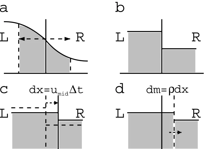
2.1 Piecewise-Parabolic Fluid Variable Re-construction . . . 54
2.2 The 1D Hydrodynamic Solver . . . 55
3.1 Lx as a Function of Roche Lobe Overflow . . . 83
3.2 Lx(t) for Full RLOF, Wind Accreting, and Transitional Cases . . . 85
3.3 Slow Rotator . . . 87
3.4 J, ˙J,Lx for the Slow Rotator . . . 89
3.5 Fast Rotator . . . 90
3.6 J, ˙J,Lx for the Fast Rotator . . . 92
3.7 The Global Hydrodynamic Model of LMC X-4 . . . 97
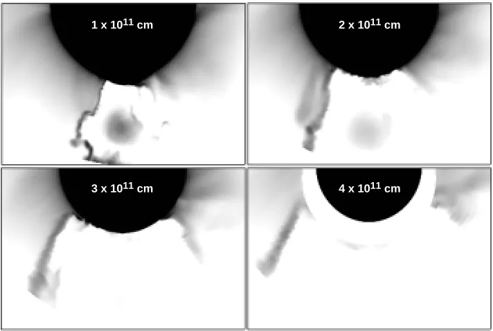
3.8 Time Series of the Circumstellar Gas . . . 98
3.9 The Five Key System Components . . . 99
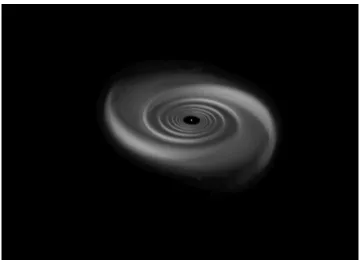
3.10 The Accretion Disk . . . 101
3.11 The Disk Wind . . . 103
3.12 Disk Wind and the Circumstellar Gas . . . 105
4.1 Computational Domain . . . 119
4.2 Spirals Waves in the Disk . . . 122
4.3 The Disk at Early Time . . . 123
4.4 The Disk at Late Time . . . 124
4.5 Formation and Vertical Instability of Spiral Shocks . . . 126
4.8 Tidal Bulging of the Outer Disk . . . 130
4.9 Epicyclic Motions of the Disk Interior . . . 132
4.10 All Cases at Late Time . . . 133
4.11 αM˙(t) . . . 134
4.12 αL˙(t) . . . 134
4.13 αWRφ(t) . . . 135
4.14 αWRφ(t) at Small Radii . . . 135
4.15 Space-time Diagram of αM˙(R, t) fon = 3 . . . 137
4.16 Space-time Diagram of αM˙(R, t) forn = 0 . . . 138
4.17 Period Doubling Behavior . . . 139
4.18 Disks With Tidal Stream . . . 141
4.19 α With Tidal Stream, n= 0 . . . 142
4.20 α With Tidal Stream, n= 15/8 . . . 144
4.21 Morphology of the Tilted Disks . . . 145
4.22 Precession of the Tilted Disks . . . 147
4.23 Evolution of the Tilt Angle . . . 148
Introduction
Consider a roller coaster. All the way through your clanking, groaning ascent to the
top of the first peak, you, your fellow passengers, and the very car you’re riding in are
being imbued with energy, gravitational potential energy. After cresting, you begin your
gut-wrenching descent. The gravitational potential energy stored within you is quickly
turned into kinetic energy as you roar around the coaster (not to mention some of the
chemical energy you stored up at breakfast being turned into acoustic energy as you
scream your head off). As you alternately climb and descend your allotted quantity
of energy is sloshed back and forth between kinetic and potential, all the while being
gradually eaten away, dissipated, by the friction of the wheels on the track heating both
up, the drag of the air you blast through robbing you to move the air, the roar of the car
being carried away on the wind. In the end, all of your last remaining supplies of your
original gravitational potential energy are abruptly ripped away in a squeal of brakes
as you stop. All of your original gravitational potential energy has been liberated and
dissipated. Your mass has been added to that of the Earth, and the energy that kept
you separate from her is now gone. This, essentially, is accretion.
Accretion according to the dictionary is “Growth or increase in size by gradual
ex-ternal addition,” but we are more interested in the liberation of energy that occurs
during this process, in other words, we are interested in accretion as a power source.
In astrophysics, many luminous sources are powered by accretion, including protostars,
cataclysmic variables, X-ray binaries,γ-ray bursters, quasars, active galactic nuclei, etc.
For our purposes, we will be concentrating on the accretion of material onto a compact
star, such as a white dwarf, neutron star, or black hole.
1.1
Accretion as a Power Source
Consider a particle of mass mat a large distancer from a star of massM and radius R.
The gravitational potential energy of the particle due to the star is −GMm/r, where
G is Newton’s universal gravitational constant. If the particle is allowed to fall freely
to the surface of the star, its gravitational potential energy will decrease to −GMm/R.
The difference is the amount of gravitational potential energy liberated during the fall,
which is converted into the kinetic energy of the falling particle. For r R, the energy
liberated becomes:
∆E =−GMm
R .
If we now “rain” material onto the star at a rate ˙M ≡dM/dt the energy liberated per
unit time is:
Lacc= dE
dt =−
GMM˙
This is the accretion luminosity. We see that the accretion luminosity depends on two
parameters, the compactness of the accretor M/R, and the mass accretion rate ˙M, and
can be tremendously efficient at liberating energy. The maximum amount of energy that
can be liberated from an amount of mass is given by Einstein’s relation E = mc2, if
the mass is entirely converted into energy via annihilation. The maximum luminosity
is then Lmax = ˙mc2. Any other process such as nuclear fission, fusion, or accretion
will have some efficiency η with which it can liberate energy, L=ηmc˙ 2. The efficiency
of thermonuclear fusion of hydrogen is 0.007, whereas the efficiency of accreting onto
a stellar mass black hole or the surface of a neutron star is about 0.1; accretion onto
such a compact object is 15–20 times more efficient as a power source than is nuclear
fusion. Accretion onto super-massive (M 109M
) black holes in AGN and quasars (whose luminosities approach and exceed 1047 erg sec−1) requires an accretion rate of
approximately 20Myr−1, compared to the burn rate of 250M
yr−1required by nuclear fusion. Considering that these sources vary on a timescale of weeks or days, they must
be contained in a volume smaller than our solar system. We see that accretion is the
only viable candidate to power these objects.
1.1.1 The Spectrum to Expect
It is important to know what we can observe about these sources, what to look for.
Typically, we expect the material being accreted is a gas; it will emit some characteristic
spectrum of radiation depending on the properties of the flow. If the emitted radiation
the photons for a long time), then the emitted spectrum would be that of a blackbody
of temperature
TBB = (Lacc/4πR2σ)1/4.
Note the dependence on the mass accretion rate (implicit in the accretion luminosity
Lacc); the more stuff accretes, the hotter it gets, which makes sense, since you are
liberating energy at a higher rate. If, on the other hand, the released energy is converted
entirely into thermal energy and the photons immediately escape (i.e. the gas is optically
thin), the thermal energy of each hydrogen atom in the gas, 32kT for the protons plus
another 32kT for the electrons, is equal to the gravitational potential energy released:
2× 3
2kTT h ≈
GMmp
R .
Hence the gas will be at the thermalized temperature TT h = GMmp/3kR. Lastly, we
will define the radiation temperature as the temperature corresponding to the energy of
an average photon: hν¯=kTrad, or Trad =hν/k¯ .
The emitted spectrum will then have a radiation temperature that falls somewhere
between the two extremes, the optically thick blackbody case, and the optically thin
thermal emission case: TBB ≤Trad ≤TT h. Using numbers for an accreting neutron star,
we find the minimum (blackbody) temperature to be about 107 K, and the maximum
optically thin temperature to be about 6×10¹¹ K. Hence we expect emission primarily
in the X-ray to γ-ray:
1 keV ≤hν¯≤50 Mev.
X-rays and γ-rays cannot penetrate the Earth’s atmosphere, so ground-based
Figure 1.1: The sky in X-rays. From the ROSAT mission, NASA. Astronomy Picture of the Day.
with rocket-borne X-ray detectors. In 1962 American Science and Engineering (AS&E)
discovered the cosmic X-ray source Scorpius X-1, the very first extra-solar X-ray point
source to be discovered, using a rocket launched detector. Dedicated X-ray telescope
launches blossomed in the 1970s with satellite such as Ariel 5, HEAO-1, SAS-3,
OSO-8, Uhuru, and arguably the most important, Einstein, launched in 1978. Ever more
sensitive X-ray telescopes have continued to be developed and launched, culminating in
recent years with satellites such as ASCA, EXOSAT, Ginga, RXTE, and ROSAT. These
missions show our galaxy and its neighbors to be veritable hives of X-ray sources, as in
Figure 1.1.
1.1.2The Effect of the Luminosity on the Flow
We have calculated that an intense flux of high energy photons will be produced by
on the accretion flow via three mechanisms: 1) radiation pressure, 2) heating (or cooling),
3) photoionization. For now, let us assume that the in-falling gas is entirely hydrogen.
The intense X-ray flux will heat the gas via scattering. If the gas becomes hot enough,
the radiation will photoionize the gas, stripping the atoms of their electrons, creating
essentially a two-fluid plasma of ions and electrons. The radiation then exerts a force
on the free electrons via Thompson scattering; the electrons in turn drag the ions along
via Coulomb attraction. This radiation pressure acts to oppose the force of gravity such
that the net force felt by the ions (which contain most of the mass of the gas) is lowered
in proportion to the luminosity:
FG=
GMmp− LσT
4πc
1
r2,
where mp is the mass of the proton (i.e. an ionized hydrogen atom), c is the speed of
light, and σT is the cross section for Thompson scattering, assuming the gas is fully
ionized.
Because of this feedback, the radiation pressure due to the accretion luminosity acts
as a throttle to the mass accretion rate. The inward force felt by a parcel of gas vanishes
for a particular value of the luminosity:
LEdd = 4πGMmpc
σT ,
the Eddington limit.
This condition need not hold in physical systems where the accretion is not spherically
symmetric, for example if accretion were to occur primarily at the star’s equator while
it does provide a rough estimate for the maximum luminosity of a star of a given mass.
For example, it can be shown that the maximum accretion luminosities of accreting
compact stars such as white dwarfs and neutron stars (both about the mass of the Sun)
are about 1038erg s−1. For comparison, the luminosity of the Sun, due to thermonuclear
fusion rather than accretion, is 3.89×1033 erg sec−1.
1.2Accretion in Binary Systems
So, do we observe compact X-ray sources that could be attributed to accretion onto
compact stars? Indeed we do; we find them in close binary star systems. They come
in several flavors, the so-called cataclysmic variables (CVs), which are believed to be
accreting white dwarfs and emit primarily in the extreme ultraviolet and soft X-ray, and
the X-ray binaries (XRBs), which are believed to be accreting neutron stars and black
holes, which emit primarily in the X-ray. All of these bright sources have companion
stars feeding them their requisite mass accretion rates ˙M via various mechanisms of
mass transfer. To understand the mass transfer and types of accretion processes in
these systems, let us consider their geometry.
For simplicity, we shall restrict ourselves (for now) to the case of two stars in circular
orbit around each other with the mass donor rotating synchronously with the binary
orbit. Circularization of the orbit and synchronous rotation within a close binary system
are expected due to tidal forces between the two stars. Consider two stars of masses M1
of:
P2 = 4π
2a3
G(M1+M2).
It is convenient to examine this system using a frame of reference that rotates with the
binary orbit. This frame rotates with an angular frequency given by:
ω2 = G(M1+M2)
a3 .
In this frame we may write an expression for the effective potential felt by a parcel of
gas. This includes the gravitational potential of the two stars, as well as the centrifugal
potential due to the rotating frame. The effective potential can then be written:
Φeff(r) = −GM1
r1
− GM2 r2
− 1
2ω
2r2 cm,
where r1, r2, and rcm are the distances to M1, M2, and the binary center of mass,
respectively. This is called the Roche potential. There exists along the line of centers
connecting M1 and M2 a point where the effective potential has zero slope, and hence
the net force vanishes. This is called the inner Lagrange point, or L1. It is a saddle
point in the Roche potential, being a maximum along the line of centers, but a minimum
transverse to it. This means that a particle displaced to the side of the L1 point will
experience a restoring force, but a particle displaced toward one of the two masses will
accelerate toward that mass. The value of the effective potential at L1 defines thecritical
potential; an equipotential surface of this potential is composed of two lobes, known as
Roche lobes, connected at the L1 point like an hourglass or dumbbell. The L1 point
acts as a throat where material can more easily move from one lobe to the other.
L1
+
*
*
cm
M
1M
2Figure 1.2: Stars M1 and M2 rotate about their common center of masscm. The critical surface of the effective potential forms the figure-8 shaped Roche lobes, connected at the inner Lagrange point, L1.
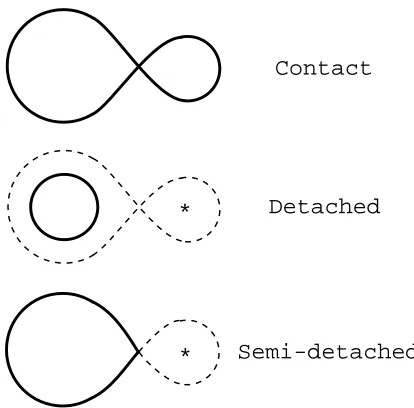
only by the mass ratio q≡M2/M1, and the orbital angular frequencyω. Depending on
the sizes of the two stars relative to their respective Roche lobes, we can classify three
distinct types of binary: contact, detached, and semi-detached. For our discussion, we
will always take the accreting star to be M1 and the donor star to beM2.
A contact binary occurs when both stars are large enough that they fill their Roche
lobes and their surfaces are essentially in contact; such systems are not expected to
survive very long in this state before evolving toward a common stellar envelope, and
becoming a single star.
Most binary systems are detached binaries. Neither star fills its Roche lobe. This
does not mean that mass cannot be transferred between the two; for example, if one
star possesses a stellar wind, this wind could be gravitationally focused and accreted by
its companion; this mechanism of mass transfer is called wind accretion.
*
*
Contact
Detached
Semi-detached
Figure 1.3: Contact binaries have surfaces that are in contact with each other, while detached binaries surfaces are well within their Roche lobes. Semi-detached binaries have only one lobe-filling star.
Material can escape from the envelope of the lobe-filling star (the donor) through the
L1 saddle point and fall toward the other star (the accretor). This is commonly referred
to as Roche lobe overflow (RLOF).
1.2.1 Wind Accretion in Detached Binaries
If a star of mass M is placed in a uniform wind of density ρ moving at speed u,
gravi-tational attraction will focus a column of wind onto the accreting star. The size of the
accretion cylinder is determined by the speed of the flow and the mass of the accretor;
in order for gas to accrete it must have kinetic energy less than the gravitational binding
energy at its (undeviated) point of closest approach:
1 2u
2 = GM
*
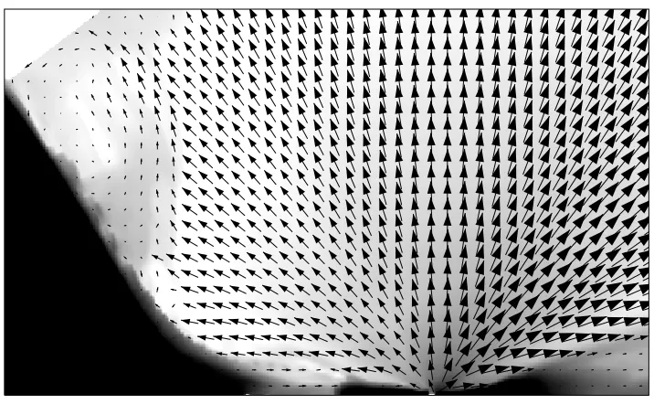
Figure 1.4: The stellar wind from the donor star (trailing in the rotating frame due to conservation of angular momentum) in this detached binary is gravitationally captured by a compact accretor, forming a bow shock.
The mass accretion rate is then ρuπr2 acc:
˙
Mwind=
4πρ(GM)2
u3 . (1.1)
This is called Bondi-Hoyle accretion [Bondi and Hoyle, 1944].
In the case of a wind fed accretor within a binary system, we expect deviations from
this ideal, as we expect there to be gradients in the density and velocity of the wind
[Taam and Fryxell, 1988]. Also, we generally expect the flow to be supersonic, implying
that a bow shock will develop ahead of the accreting star. The bow shock may effect
the accretion rate, as some of the kinetic energy will be dissipated crossing the shock,
meaning that a larger gas column may accrete, but back pressure behind the bow shock
may be strong enough to choke accretion. The precise result will of course depend on
the detailed dynamics of the interacting wind and shock, including radiative heating and
cooling [Taam et al., 1991]. In the ideal case, we expect no net accumulation of angular
change this. Still, Equation 1.1 provides a rough constraint on the wind for systems
whose luminosity is believed to be powered by wind accretion.
1.2.2 Roche Lobe Overflow
Lubow and Shu [1975] and Lubow and Shu [1976] form the foundation of our
under-standing of mass transfer in semi-detached binaries. In these systems, the surface of the
Roche-filling star is essentially unbound at the L1 point; the thermal gas pressure will
force material through the saddle point in the Roche potential at the sound speed
(im-plying that as the stream accelerates toward the accretor the flow is always supersonic).
We thus expect the formation of a stream of material from the surface of the donor star.
We call this the tidal stream. From the accreting star’s point of view, the L1 point lies
at a distance rL1 that depends on the mass ratio of the system, and rotates about the
accretor with angular velocity ω. The gas then contains an angular momentum per unit
mass given by ωr2L1. In other words, this stream of material cannot fall straight into the
accreting star; it is in orbit.
Without interference, a particle released from the L1 point will follow a ballistic path
around the accretor, passing closest to it at some periastron point. If the radius of
the accretor is smaller than the radius of this periastron, the stream gas will continue
to orbit, eventually intersecting other stream material. We may expect these colliding
gas flows to circularize at a radius given by a Keplerian orbit with specific angular
momentum ωrL21:
*
rcirc rmin
Figure 1.5: The photosphere of the donor star is unbound at the L1 point, and forms a gas stream that pours into the compact star’s Roche lobe. This stream enters the Roche lobe at the sound speed (since it is gas pressure that pushes it through the L1 point), and accelerates toward the accretor. The supersonic flow follows a ballistic trajectory, passing the compact star at a radiusrmin before colliding and circularizing at radiusrcirc.
For example, in a system withq= 1 (equal mass stars), whererL1/a= 1/2,rcirc/a= 1/8.
If angular momentum were conserved this gas would form a torus at the circularization
radius. If angular momentum can diffuse outward while gas can drift inward, then a
disk is formed. This configuration is known as an accretion disk.
For the case of accretion onto a compact object, the point of closest approach of
the stream is less than the circularization radius of the incoming material; it stands to
reason that the stream will have to strike the disk in these systems. Since the gas stream
starts out its journey from the L1 point moving at the sound speed (remember, it leaks
through the L1 point due to thermal pressure from the donor’s photosphere) and is in
free fall toward the accretor, we expect the stream material to be supersonic when it
strikes the disk. We may expect strong shocks at this high velocity impact, heating the
gas via dissipation, creating a hot spot. However, this may not always be the case; if
the impact is sufficiently oblique, or the ratio of the density of the disk to the stream
disk to accrete matter slowly), or the gas stream is only just supersonic (as may be
the case in very low mass ratio systems, where the disk may extend nearly to the L1
point) then emission by a hot spot may be diminished. Splashing of stream material at
the disk edge, or expansion of the disk edge due to heating by the stream impact, may
contribute to phase-dependent modulation of flux from the accretor by increasing the
column density of material along our line of sight to the source at certain phases.
1.2.3 Binary Evolution
Binary stars over their lifetimes may experience different epochs during which mass
transfer occurs or does not. Also, the same binary star may experience multiple types of
mass transfer during its evolution. For example, a star may begin to drive a wind during
one evolutionary phase, leading to wind-fed accretion onto its companion. This same
star may evolve to a larger radius, filling its Roche lobe, leading to RLOF. The binary
separation of the system will decrease over time as orbital angular momentum is carried
away in a stellar wind, which may act to drive wind-fed systems toward RLOF. We may
then see wind accretion and RLOF as the two extremes in a continuum of mass transfer
states. We may ask ourselves, what is the transition like between these two extremes?
How sharp is this transition, and are we able to identify any likely candidates to be in
this regime? Later in this work, we define the Roche lobe overflow parameter λ, which
is a measure of the “filling factor” of the donor star; i.e. how close it is to filling its
Roche lobe, and examine the role it plays in determining whether a given system will
Another factor affecting the mode of mass transfer is orbital eccentricity; although
circularization is usually a good assumption, exceptions are known. Within the X-ray
binaries, one of the two stars will be a collapsed object that will have lost a significant
fraction of its mass explosively. This process is expected to alter the eccentricity of
the binary orbit, and circularization of an elliptical orbit will take some amount of
time, during which we may observe an X-ray binary in non-circular orbit. The elliptical
orbit X-ray binary GX 301-2 provides an excellent laboratory for investigating many of
the typical assumptions about X-ray binaries, as well as unique phenomena, since the
accreting neutron star periodically plunges deep into the companion star’s stellar wind,
very close to the companion. This essentially forces the system to undergo Roche lobe
overflow once every binary orbit (see Chapter 3).
1.3
Accretion Disks
We may understand some important concepts about accretion disks merely from first
principles. We know that the gas flow will involve dissipative processes such as shocks
that will heat up the disk. Radiation will carry energy away from the disk in the form of
a disk luminosity; in other words, the disk will shine. The ultimate source of the disk’s
luminosity must be liberated gravitational potential energy, i.e. some portion of the gas
in the disk must move inward. But for this to occur, angular momentum must be lost
in order for a gas parcel to drop to a lower orbit. Typically, angular momentum transfer
involves internal torques within the disk and takes place much more slowly than energy
given angular momentum, meaning that the gas orbits are likely near-circular (circular
orbits have the lowest energy in the absence of the perturbation of the companion’s
gravity), with gas slowly spiraling inward as potential energy is liberated and angular
momentum is transported outward. In order for angular momentum to be transported
outward some fraction of the disk gas must carry it out. This implies that the outer
disk spirals out while the inner disk spirals in.
Circular orbits imply that the gas flow isKeplerian: vkep =GM/r. In the case of
an accretion disk, material that falls onto the surface of the accreting compact object
impacts with grazing incidence with specific energy−GM/R+12v2kep =−12GM/R. For
a mass accretion rate ˙M, the disk luminosity is then half the total accretion luminosity:
Ldisk = GM ˙
M
2R =
1 2Lacc.
The other half of the accretion luminosity is either liberated at the accretor’s surface,
or may be lost in the case of a black hole accretor, which has no rigid surface for the
accretion flow to impact.
Since the operation of our accretion disk as a machine for energy extraction depends
on the transport of angular momentum, it behooves us to examine how such transport
may take place.
1.3.1 Viscous Transport
The astute reader will notice where the hand-waving has occurred: in the transport of
angular momentum. How exactly is angular momentum transferred through the disk?
of the gas, which varies inversely with the square root of the radius. This means that
gas orbiting at smaller radii is moving faster, and gas orbiting at larger radii is moving
slower. Imagine that two successive annuli of the disk rotate as rigid hoops with the
appropriate Keplerian orbital velocity. Now imagine that each hoop exerts some drag on
the hoop next to it. You can see that the fast moving inner hoop will act to speed up the
slow moving outer hoop, and vice versa. In other words, the drag between concentric
annuli (viscosity) acts to transfer angular momentum from the inner annulus to the
outer one. The inner annulus, now moving at sub-Keplerian velocity for its radius, will
fall inward, accelerating until it reaches equilibrium. The outer annulus, now moving
at super-Keplerian velocity for its radius, will move outward. Hence viscosity within
the disk allows angular momentum to be transferred outward while mass moves inward,
liberating gravitational potential energy.
Consider now two neighboring annuli of width δr sharing the surface of radius r,
assuming the disk to be in equilibrium. We can see from the Keplerian flow that the
inner annulus will be moving faster than the outer annulus, just as in our two-hoop
model. The chaotic motions of the fluid ensure that fluid elements are continually
exchanged across the surface at radius r with characteristic speed ¯v. Elements moving
outward will carry an average angular momentum density of ρ(r−δr/2)2Ω(r−δr/2),
while fluid elements moving inward will carry an average angular momentum density of
ρ(r+δr/2)2Ω(r+δr/2), where Ω(r±δr/2) is the average angular velocity of the Keplerian
flow within the two annuli. Because we have restricted the flow to be in equilibrium,
Figure 1.6: Two neighboring annuli in a Keplerian accretion disk exchange fluid elements in equilibrium. The net mass flux is zero, but the fluid elements from the inner annulus carry different angular momentum than do those from the outer annulus. Hence a net angular momentum flux exists, exerting a torque that acts to slow the inner annulus and speed up the outer one.
non-zero. Let the disk have a thickness H. The net angular momentum flux is then
2πrρvH¯ (r−δr/2)2Ω(r−δr/2)−(r+δr/2)2Ω(r+δr/2),
or perhaps more clearly, since r δr:
−2πr3Hρvδr¯ Ω(r+δr/2)−Ω(r−δr/2)
δr .
The fraction is just Ω = dΩ/dr, while we may define ρH ≡ Σ, the surface density, or
the mass per unit surface area, of the disk. We will also define the standard coefficient
of kinematic viscosity ν ≡ vδr¯ (also called the shear viscosity). Hence the net torque
(the rate of change of the angular momentum) of the inner annulus on the outer annulus
is
τ(r) = 2πr3νΣΩ.
Meanwhile, the work on an annulus of the disk betweenrandr+drby the net torque
due to its neighboring annuli (interior and exterior) is
Ω∂τ
∂rdr= ∂
∂r(τΩ)dr−τΩ
dr.
energy through the disk via the torque; this energy can only have sources or sinks
according to the boundary conditions at the inner and outer edges of the disk. But the
second term,−rΩdr, represents a local energy sink; the torques act to dissipate the gas’
mechanical energy, which must go into internal energy, heating the disk. This loss of
mechanical energy, which can only come from the gas’ rotational energy, is what drops
the gas to a lower orbit, liberating gravitational potential energy in order to speed the
gas back up to Keplerian velocity.
We see then that the efficiency of the disk in communicating angular momentum,
and hence its efficiency as a machine for extracting gravitational potential energy, is
dependent upon the viscosity ν. What then can we say about the magnitude of ν?
Unfortunately, we can say a lot.
Let us consider the Reynolds number of the flow, which is a measure of the relative
importance of the inertia of the fluid flow to the viscosity:
Re= rvφ ¯
vδr.
If Re 1, viscous forces dominate the flow (as in motor oil). If Re 1, viscosity
is unimportant. Using typical values for the size and speed of flow expected within
accretion disks, and taking δr and ¯v to be the mean free path between collisions and
the sound speed of the gas, respectively, we find that the molecular Reynolds number
exceeds 1014, making the normal kinematic viscosity completely negligible. Molecular
viscosity cannot extract the energy we require.
However, the large magnitude ofRemol seems to imply that it is likely that accretion
Turbulent flow is characterized by large scale chaotic motions. ¯v andδr now become the
turnover velocity and size of the largest turbulent eddies within the flow. Unfortunately
our ignorance of turbulent fluid flow is profound. We cannot state a priori at what
point the hypothetical turbulence would saturate, since this would depend on unknown
physical mechanisms within the disk. We can provide an upper limit for both δr and
¯
v at best. We know that the size of the largest turbulent eddies cannot exceed the
thickness of the disk, so δr ≤ H, and we know that the turbulent velocities are likely
not supersonic, since if they were the turbulent motions would be dissipated away by
shocks, so ¯v ≤cs, where cs is the sound speed.
Hence we parameterize all of our ignorance in the infamousα−prescriptionof Shakura
and Sunyaev [1973]
ν≡αcsH,
where we expect on the previously stated physical grounds that α <1.
Unfortunately for us, recent work by Balbus and Hawley [1998] shows that the radial
gradients in the Keplerian flow act to stabilize it; indeed the disk isnot hydrodynamically
turbulent. However, we note that molecular interactions or hydrodynamic turbulence
need not be the only physical mechanisms that can create viscosity within the disk.
Any mechanism that can couple the shearing flows within the disk, and hence transport
angular momentum, will act like a viscosity. One promising mechanism is the so-called
magneto-rotational instability, or MRI, of Balbus and Hawley [1998]. Consider two
magnetized fluid elements rotating in neighboring annuli. If the disk is in Keplerian
But the tension in the magnetic field between the two elements acts as a spring, coupling
the two elements, that is being stretched. The inner element will be slowed, and the
outer element will be accelerated, i.e. angular momentum is transferred from the inner
element to the outer element. The inner element falls in while the outer element moves
out, exactly as in our previous example. Thus the MRI provides a magnetohydrodynamic
viscosity to the disk.
1.3.2Non-Viscous Transport by Global Waves Modes
All of the angular momentum transport mechanisms we have discussed so far have been
local effects; in other words effects that are dependent only on local quantities within
an infinitesimal portion of the disk and behave like a fluid viscosity. However, angular
momentum can be transported by completely non-viscous effects such as global wave
modes (Goldreich and Tremaine [1980]; Lynden-Bell and Kalnajs [1972]; Papaloizou
and Pringle [1977]), such as spiral shocks, which can act as an angular momentum sink
(Larson [1989]; Sawada et al. [1986b]; Shu [1976]; Spruit [1987]). Consider a shock within
the disk at some obliquity to the fluid flow. As the flow crosses the shock, some portion
of its mechanical energy is dissipated, heating up the disk. Hence a gas parcel crossing
this shock loses rotational kinetic energy, and will fall toward the accretor, liberating
gravitational potential energy. This argument depends, of course, on whether or not the
angular momentum carried by the fluid element can be carried away.
Up to this point we have assumed the flow of our accretion disk to be Keplerian.
from the disk’s point of view, orbits it. Just as the gravity of the moon orbiting the earth
distorts the fluid covering the earth (the oceans) causing high and low tides, the orbiting
presence of a massive companion causes tides within an accretion disk. Consider again
the disk in a frame rotating with the binary. The gravity of the companion, as well as the
centrifugal and Coriolis forces due to the rotating frame, will vary with azimuth around
the disk. This implies that the equilibrium orbits of the disk are no longer Keplerian.
Paczynski [1977] identifies a family of closed pseudo-elliptical orbits that are solutions
to the restricted three-body problem (in absence of pressure forces) in the region of the
accretor. Differential accelerations around the disk due to the tidal forces will cause some
regions of the flow to move faster than others; the flow will develop over-dense regions
where the flow is slower, as well as rarefied regions where the flow is faster. These
disturbances are sheared out by the Keplerian flow into spirals, and pressure gradients
in the flow will steepen them into shock waves as they propagate inward. These are the
famous two-armed trailing spiral shock waves of accretion disks in binary systems. Let
us examine them in detail.
The equilibrium position of the spiral shock is determined by a balance between the
ram pressure ahead of the shock and the gas pressure behind it. Since the ram pressure
ahead of the shock is proportional to the speed of the flow perpendicular to the shock
squared, and the speed of the flow increases with decreasing radius, we see that the
obliquity of the shocks must increase to keep the ram pressure of order the gas pressure.
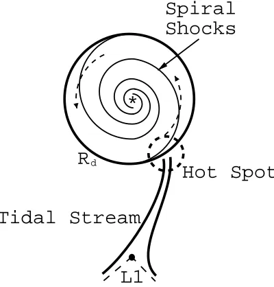
Hence, the spirals become more tightly wound at smaller radii:
*
Hot Spot
Tidal Stream
Spiral
Shocks
Rd
L1
Figure 1.7: The accretion disk’s outer radiusrD is greater than the circularization radius,
due to the outward flux of mass and angular momentum. The outer radius lies at the
or
sinθ ∝ 1
M,
where θ is the shock angle (the angle between the pre-shock flow and the shock) andM
is the Mach number of the flow, v/cs. Since the shock can only dissipate kinetic energy
from the component of the velocity perpendicular to the shock, this implies that the
spiral shocks become less and less efficient at dissipating energy at small radii, since this
component becomes ever smaller. Eventually, the shock is wound so tightly that the
flow is all but parallel to the shock, and the shock essentially ceases to exist. In other
words, dissipation by the spiral shocks turns off at smaller radii. If the Mach number
of the disk is large enough everywhere, dissipation by spiral shocks will be negligible
throughout the disk.
The spiral shocks are two armed because the disturbance that creates them, the tidal
forces, is an m = 2 mode (to first order). Shu [1976] postulate that the impact of the
tidal stream could drive a one armed spiral into the disk, since there is only a single
propagating disturbance (the impact) to be sheared out by the flow; this m = 1 mode
should drive accretion in the same manner as the tidally driven m = 2 spiral modes.
Hence it is possibly that the actual disk structure may have both one and two armed
spiral modes propagating through it.
1.3.3 Tilted Disks, Precession, & Radiation Torque
There is considerable observational evidence that some systems contain tilted, precessing
tilted disk, and how it might get that way.
Consider an accretion disk that orbits in a plane other than that of the binary orbit.
The orbits of this disk experience non-symmetric tidal forces around the disk; thus
each annulus of the disk will experience a tidal torque (this is true whether the disk
is tilted or not). Consider a top that is spinning about an axis off the vertical. The
gravitational force causes the top to experience a torque that is perpendicular to the
angular momentum vector; the magnitude of the angular momentum stays the same,
but the direction changes; i.e. the axis of rotation of the top precesses. Similarly, tidal
torques will cause the direction of a tilted disk in a close binary to precess. Because
the accretion disk is a fluid, communication of the tidal torques makes the precession
rate relatively independent of radius (in other words the disk precesses more or less
coherently, as though it were a rigid body), while the net torque depends on the outer
radius of the disk, where the tidal forces (and hence the torques) are strongest. Larwood
shows that the ratio of the orbital period to the precession period is
Porb Pprec = 3 7 q2
1 +q
1/2 Rd
a
3/2
cosi. (1.2)
where Rd is the radius of the accretion disk, and i is the inclination of the disk relative
to the binary orbital plane (i= 0 is in the binary orbital plane) [Larwood, 1998a].
Katz [1973] proposed periodic obscuration by a precessing tilted accretion disk to
explain recently-discovered super-orbital periodicities observed in the light curves of the
X-ray binary Her X-1. Roberts [1974] proposed a “slaved disk model” in which the donor
star rotates with an angular momentum vector misaligned with the binary orbital angular
misaligned angular momentum vector. However, the net angular momentum transferred
over an orbital period is still aligned with the binary orbital angular momentum, since
half the time the accretor is above the donor’s equator, and half below; the residence
time of the disk gas would have to be extremely brief. Also, the axial tilt of the donor
would decay due to tidal friction on a timescale shorter than the orbital circularization
timescale, and Her X-1 is believed to be circular or near-circular.
The likely candidate is thought to beradiation driven warping. Motivated by
Petter-son (PetterPetter-son [1977a]; PetterPetter-son [1977c]; PetterPetter-son [1977b]) and Iping and PetterPetter-son
[1990], Pringle [1996] showed that a centrally illuminated disk is unstable to warping by
re-radiation back-pressure. To understand how radiation driven warping works, we need
to understand how the disk is illuminated by the central source.
Consider an accretion disk that is everywhere in local hydrostatic equilibrium. For
a given fluid element at some small distance z (the disk is thin) above the binary
or-bital plane, the cylindrical-radial component of the accretor’s gravity is balanced by the
centrifugal force (we shall neglect the companion for the moment):
GM R2
r
R =
v2 φ r ,
where R is the distance to the accretor and r is the cylindrical radius. Since the disk is
thin, we arrive at the familiar Keplerian velocity profile:
vφ(r)≈
The disk is supported vertically against collapse due to the accretor’s gravity by
hydro-static equilibrium:
fz =−GM
R2 ρ z
R −
dP dz = 0.
For convenience, consider an isothermal equation of state P =c2
sρ. Rearranging we find: dρ
ρ =−
GM c2
sR3 z dz,
or
ρ(z) = ρ0e−z2/H2,
where H is the scale height of the disk, i.e. its thickness, and is defined by
H2(R)≡ 2c
2 s
GMR
3.
We see that the thickness of the disk increases with increasing radius as the 3/2 power,
thus the disk is concave.
Because of this concavity the disk surface will intercept some amount of flux from
the central source. In the case of an accreting neutron star or black hole in an X-ray
binary, that flux will be mainly hard X-rays. Since the X-rays are traveling radially,
direct radiation pressure can exert no torque on an orbiting fluid annulus that absorbs
them. However, they can and do heat up the disk surface, causing re-radiation of the
reprocessed X-ray flux. Since this re-radiation is preferentially normal to the disk surface,
it can exert a torque on the surface. Since the disk has two surfaces, one might expect
that the net torque would remain zero, but Pringle has shown that even an initially flat
disk is unstable to radiation torques if the central source is sufficiently luminous [Pringle,
*
Figure 1.8: The concavity of the accretion disk’s surface implies that it will be strongly illuminated by the central X-ray source. While the direct X-ray flux can exert no torque, the force due to thermal re-radiation of absorbed X-rays is normal to the surface, and can exert a net torque. The disk is unstable to warping via this mechanism if the central luminosity is high; once the symmetry is broken and opposite surfaces become shadowed on opposite limbs of any annuli, torques can easily warp the disk.
Such radiation torques can drive the disk out of the plane, tilting and twisting it,
creating a warped disk. Once out of the plane, radiation and tidal toques will induce
precession of the disk, yielding super-orbital periodicities via cyclic changes in the
ori-entation of the system over time. Even though the primary must orbit the tilted disk
once every binary orbit, the particular orientation of disk and companion as a
func-tion of phase now changes for us, the observers. At one point, the disk may be facing
us, providing an unobstructed view of the hard X-ray source (excepting eclipses by the
companion), in other words a “high” state, while at some time later, precession of the
disk may obscure the hard X-ray source completely behind the edge of the disk, leaving
only coronal emission or perhaps cold X-ray reflection from the companion, i.e. a “low”
1.4
Observing Accretion onto Compact Objects in Close
Bina-ries
We have built up a rather extensive catalog of physical possibilities for accreting systems
in binary stars. Let us now examine the observational evidence for them. Indeed we do
see a plethora of galactic and near-galactic point X-ray sources which can be attributed
to accretion onto a compact object in a binary star. Generally, these fall into three
classes: the high mass X-ray binaries (HMXBs), the low mass X-ray binaries (LMXBs),
and the so-called cataclysmic variables. The first two collectively make up the XRBs. In
this section we will examine both the observational classes, and the various observational
techniques used to investigate them.
1.4.1 Nomenclature
Let me first digress and discuss X-ray source naming conventions. Historically, point
X-ray sources are identified by the constellation they occupy and an X designation
signifying their brightness relative to other X-ray sources in that constellation; Her X-1
is the brightest X-ray source in the constellation Hercules. Near-galactic sources in the
Small and Large Magellanic Clouds receive SMC and LMC designations; hence LMC
X-4 is the fourth brightest X-ray source in the Large Magellanic Cloud. Fainter sources
*
a
b
c
d
Figure 1.9: At high inclination (a), the hard X-ray source is obscured by the disk and only scattered or reflected X-rays, or X-rays emitted from a hot diffuse corona above and below the disk, can be seen. At slightly lower elevations (b) the hard X-ray source can be seen, with the flux modulated by the outer edge of the disk. Eclipsing will be observed up to point (c), the position of which depends on the mass ratio of the system (and hence the relative sizes of the disk and donor). Specific features of the system structure such as attenuation of X-ray flux by a splashing impacting tidal stream may be observed up to moderate inclinations (d) beyond which only the hard X-ray source can be seen.
1.4.2Geometric Considerations
We may predict some observational properties of accreting binary systems simply due
to the geometry of our problem, as in Figure 1.9. The binary will orbit is a plane that
makes some angle, called the inclination, with our line of sight. If we are observing
in the plane of the orbit, we should observe the disk and its donor periodically eclipse
each other as they rotate. If we are looking straight down toward the orbital plane, we
should observe no eclipsing. Since both the donor and the disk have physical extent, we
expect that the shape of observed light curves will vary according to the inclination of
the system; for example, for certain inclinations the disk or donor may partially, rather
1.4.3 Observational Techniques
We do not have the luxury of studying accreting binaries from close up; rather we must
rely solely on the photons that wend their way to our various instruments. Furthermore,
these systems are much too far away to be directly imaged. Therefore astronomers have
developed clever ways to massage the photons into divulging information about these
systems. Our entire understanding of accreting binaries comes from the interpretation
of time dependent continuum and line emission via various observational techniques.
Light Curves and Total Flux
We are interested in the time-dependent flux from the system, or the light curve.
Typically, observations of binary stars are made as a function of orbital phase, which is
essentially time, normalized to the binary period. Hence phases 0 and 1 correspond to
mid-eclipse (although some authors use the opposite convention) of the accretor (this
definition is clearly problematic if no eclipse exists). The timescale of the variability
tells us the physical scale of the source of the variability. Very rapid fluctuations in hard
X-ray luminosity likely arise near the accretor. Longer term, but still short, fluctuations
in soft X-ray or UV may correspond to the dynamics of the disk. Changes on the
orbital timescale such as eclipses give us information about the global structure of the
binary. Very long timescale variations (longer than the orbital period) may tell us about
the global evolution of the system, as we shall see later. If a distance to the object
can be determined, total flux measurements allow us to ascertain the system’s absolute
Spectra
The detailed spectra of a system can provide a wealth of information; we may expect
to identify red-shifted and blue-shifted emission due to both the binary rotation and
the rotation of the accretion disk, should one exist. We expect that different regions of
the system will have different temperatures, optical depths, ionization states, etc. and
will be emitting different spectra. Soft X-rays can provide column densities within a
system, while UV line profiles can provide stellar wind parameters. We expect different
systems (for example accreting neutron stars vs. black holes) to be emitting primarily
in different bands from UV to soft X-ray, hard X-ray, and γ-ray.
Line Profiles
Cataclysmic variable (see below) accretion disks have strong emission lines of
hy-drogen and helium. An individual line will be convolved into a complex curve by the
dynamics of the system. Consider a single line that is emitted uniformly by a disk with
some inclination to our line of sight. The rotation of the gas of this disk will cause some
of the emission to be red-shifted (when gas is moving away from us) and some to be
blue-shifted (when gas is moving toward us). Furthermore, because of the differential
rotation of the gas, the fast moving gas near the center of the disk will be shifted more
than will the slower moving gas in the outer disk. Now add in the fact that the entire
disk is in orbit around another star, adding a background shift that moves from blue
to red over the course of an orbital period. Finally, consider that it is unlikely that the
disk actually is emitting uniformly; there is no reason a priori to assume that the disk
regions where dissipation occurs, such as shocks, for example from a tidal stream impact
or spiral shocks. But we can say that generally a line from an accretion disk is expected
to be “two horned” with a red-shifted and a blue-shifted peak. Over the course of a
binary orbit, the background frequency shift due to the orbital motion will alternately
make one peak stronger than the other.
Eclipse Mapping
If we are lucky enough to observe the system at a high enough inclination, we may
observe eclipses of the disk emission by the primary. In this case, as the system enters
eclipse, the blue-shifted peak is lost, as the disk gas moving toward us is obscured. As
the system nears the end of eclipse, the red-shifted peak is temporarily lost, as the gas
moving away from us is occulted. This leads directly to a technique known as eclipse
mapping. This method is used to attempt to map out the continuum emission of the disk
surface. The continuum emission of the disk will be a complex function of the detailed
local physics of the disk, including dissipation, dynamics, radiative transfer within the
disk, etc. For example, at high energies (shorter wavelength) the emission is expected
to be sharply peaked near the accretor, while at lower energies (longer wavelengths)
the emission is more uniform. There may be localized emission at some wavelengths
due to a “hot spot” (stream impact). As the companion orbits it will eclipse different
regions of the disk surface at different orbital phases. This allows us to infer the net
emission from the region in shadow by what has beensubtracted from the signal. These
time dependent spectra may then be deconvolved to provide emission maps of the disk
*
Figure 1.10: If the inclination is high enough for the donor to occult the disk, then we may use time dependent light curves and spectra to deconvolve the emission structure of the disk.
Trailed Spectrograms & Doppler Tomograms
Returning to line emission, we may make use of the fact that the line profiles change
as a function of binary phase (and are typically different for different lines, since as we
have discussed, emission is not expected to be uniform over the surface of the disk).
Essentially, every parcel of gas in the disk will have some component of velocity along
our line of sight, producing a frequency shift. The integral over the disk surface produces
the double-peaked line profile we have already discussed. As the binary orbits, we are
essentially viewing the disk from all azimuthal angles. Stacking of line profiles over
time allows us to create a trailed spectrogram that shows the changes in the frequency
shifted line as the binary orbits. Using the same idea of deconvolving our data given
certain assumptions about the disk (namely inclination and the assumption that the
disk is Keplerian or nearly so) we may produce velocity-space maps of the disk, known
*
wavelength intensity
*
*
*
*
1.4.4 Kinds of Accreting Close Binaries with Compact Objects
We now turn our attention to the three kinds of accreting close binaries that contain
compact accretors: the X-ray binaries, including the high-mass and low-mass XRBs
(HMXBs and LMXBs, respectively), and the so-called cataclysmic variables.
High Mass X-Ray Binaries
The HMXBs are composed of giant or super-giant stars accreting onto either neutron
stars (LMC X-4) or black holes (Cyg X-1), either via wind accretion (Vela X-1), or
disk accretion (Her X-1). Typically these systems have mass ratios q > 1, usually
significantly greater than 1; for example the HMXB LMC X-4 has a donor to accretor
mass ratio of 10.6. Generally these systems have extremely high hard X-ray luminosities
(1035 − 1038 erg s−1) that are expected to be generated very close to the accretor’s
surface. Typically, ultraviolet flux from the disk is totally swamped by the luminosity
of the companion giant, which is also of order 1038 erg s−1 and is peaked in the UV.
However we know that the only process capable of generating such X-ray luminosities
is accretion onto a compact object, and it is reassuring that we can often identify an
optical counterpart, the donor star (for example, the donor star to Her X-1 is HZ Her).
Since the size of the donor star is large compared to the binary separation in these
systems, they typically exhibit eclipses of the X-ray source. Because the companion star
is generally luminous enough to be detected, we can often observe details of its stellar
envelope, such as the presence of a stellar wind by shifted absorption and emission lines
We may differentiate the wind accretors from the disk accretors in two ways. One,
the disk fed HMXBs are typically more luminous than the wind fed HMXBs, and two,
the rate of change of spin of the neutron star is typically higher in disk fed systems. If
the emission from the surface of the neutron star is not axisymmetric about the axis
of rotation, for example if matter is channeled along magnetic field lines to an off-axis
“cap” where the X-rays are then preferentially emitted, then we will observe pulses in
the neutron star’s emission as it rotates, i.e. an X-ray pulsar. Since material accreting
from a disk is expected to carry some net angular momentum, we expect the neutron
star to “spin up” over time. In a wind fed system gas from the companion’s stellar
wind is focused head on and is expected to carry little net angular momentum; hence
we expect little coherent long term change in the spin of a wind fed pulsar (although it
may be possible to form transient accretion disks behind the bow shock of a wind fed
accretor).
Low Mass X-Ray Binaries
The LMXBs are composed of an accreting neutron star in close binary orbit with a
low mass main sequence companion, typically less than 1 M. Typically the donor star
is at most about the same size as the accretion disk, and may be significantly smaller;
eclipses of the hard X-ray source are rare in these systems, since they have to be viewed
almost edge-on to produce them. Typically emission from the accretor, the disk, and
the companion all lie in different bands: X-ray, UV, and optical, respectively. However,
the companion stars are typically so faint that they are rarely detected, and the disk
emission from the disk itself.
In both classes of XRB our observational options are limited. With the exception
of the spectrum of the companion stars in the HMXBs, we are typically restricted to
measurement of the hard X-ray flux from the accretor, the reprocessed X-ray flux from
the illuminated surface of the disk or companion, or X-rays emitted from a hot corona
above the surface of the disk (an extended, rather than point X-ray source). These are
still very useful tools, however; it is as if we are able to take an X-ray of the circumstellar
gas of our binary star. Unfortunately, we are restricted to a single inclination angle for
any one system. This gives rise to a number of distinct observational clades that depend
upon inclination, as mentioned above (see Figure 1.9).
Cataclysmic Variables
This is actually a catch-all class that includes novae, dwarf novae, nova-like variable
stars, intermediate polars, etc. We will not be discussing the manifold differences of
these systems, but let us examine what they have in common. All of these system have
a normal “quiescent” luminosity that is believed to be driven by accretion from a low
mass main sequence binary companion onto a white dwarf, punctuated by periods of
higher luminosity (outbursts) that are generally attributed to sudden changes in mass
accretion rate.
Our observational options are much greater with the CVs than with the XRBs.
Be-cause of the lower compactness M/R of the accreting star, these systems are much less
luminous than the XRBs, and their emission is not dominated by the central accretor;