Improvised Spectral Clustering Using Matrix Balancing In Image Segmentation

Improvised Spectral Clustering Using Matrix

Balancing In Image Segmentation

Deepa Viswam

and Anish Abraham

1 _{M Tech Student, Dept. of CSE, Government Engineering College, Thrissur, Kerala, India} 2_{Assistant Professor, Dept. of CSE, Government Engineering College, Thrissur, Kerala, India}

ABSTRACT: Image segmentation partitions the image into multiple segments which consists of pixels with similar properties. In this work, a data clustering method called as spectral clustering is used for image segmentation. Spectral Clustering (SC) algorithms utilize top eigenvectors of normalized Laplacian matrix for spectral rounding. When local scaling is introduced in SC, clusters of the data which includes multiple scales as well as those placed within a crowded background can be separated efficiently. An average alignment criterion for selection of relevant eigen vectors can be used for finding the number of groups automatically. Along with these properties, balancing matrix which can reduce norm of matrix also leads to improve the accuracy of computation. When this property is used in Laplacian matrix of spectral clustering algorithm, this will increase the performance of clustering. Experimental results on standard dataset show better segmentation results than other improvised spectral clustering algorithms.

KEYWORDS: Eigenvector selection; image segmentation; Laplacian matrix; matrix balancing; spectral clustering. I. INTRODUCTION

Image segmentation is the process of dividing an image into meaningful structures. It is an initial step in image analysis process. It is useful in many applications [1] [2] like content based image retrieval, medical imaging, object detection and recognition tasks. Segmentation poses several challenges, [3] as the number and type of relevant elements depend on the purposes of human observation and semantic scope with global and local geometrical, textural and statistical properties of the image. Tests performed on large groups of subjects asked to perform segmentation of the same images show that segmentation results produced by humans may differ significantly. Therefore, it cannot be expected that a single segmentation procedure would yield a satisfactory result to all types of images. This explains the large number of segmentation methods presented in the literature, as , edge-based segmentation, region-growing method, clustering methods (k-means, fuzzy C-means), split and merge, thresholding segmentation based on classification of pixels according to their intensity and based on graphs, wavelets, and other hybrid methods. In this research work , image segmentation using graph based data clustering called spectral clustering is discussed.

Spectral clustering is the clustering method that treats the data clustering as a graph partitioning problem without making any assumption on the form of the data clusters. This clustering method refers to a class of techniques which rely on the eigen structure of a similarity matrix to partition points into disjoint clusters with points in the same cluster having high similarity and points in different clusters having low similarity. The process of finding good clusters has been the focus of considerable research in machine learning and pattern recognition. The problems of image segmentation and grouping remain great challenges for computer vision. Spectral clustering is a good clustering method for image segmentation. But SC algorithm still expects improvements because even though different algorithms exist, the relationship between the matrix spectrum and eigen vectors is not clear and most of the existing spectral clustering algorithm need a given number of clusters in advance.SC algorithm should face and solve two main problems. they are how to calculate the similarity and dissimilarity between datasets and how we can do the optimal partition quickly and efficiently. The existing algorithm can only solve a set of problems because of the actual complexity and the data diversity

of segmenting a digital image into a set of disjoint regions is addressed such that each region is composed of nearby pixels with similar colors or intensities.

II. RELATED WORK

A. Spectral Clustering

Spectral clustering algorithm combines data mining, Pattern recognition, mathematics, images and many other areas of research. It can be solved efficiently by standard linear algebra software [5][6][7]. It is assumed that the data consists of n points x1,…, xn which can be arbitrary objects. It is measured their pair wise similarities 𝑠𝑖𝑗 = 𝑠 𝑥𝑖, 𝑥𝑗 by some

similarity function which is symmetric and non-negative, and it denotes the corresponding similarity matrix by

𝑆 = 𝑠𝑖𝑗 _{𝑖,𝑗 =1…𝑛}.

The idea of spectral clustering algorithm is originated from spectral graph partitioning theory. It considered clust-ering as a problem of undirected graphs multi-way partitioning. Spectral clustclust-ering algorithms consist of two steps: [8] 1. Construct a similarity graph with some kind of similarity function

2. Find an optimal partition of the graph and cluster the data points. The former which reflects the intrinsic structure of the data plays an important role in spectral clustering, thus a great deal of effort has been carried out to address it. B. Normalized spectral clustering based on symmetric matrix

The normalized spectral clustering is as follows [7] [5]:

Input: A set of points S∈Rn x n , S={s1, ...,sn}, number k of clusters to construct

Step 1: Form the affinity matrix 𝐴 ∈ 𝑅𝑛 ×𝑛 _{defined by 𝐴}

𝑖𝑗 = exp⁡(−∥ 𝑠𝑖− 𝑠𝑗 ∥2/2𝜎2) if 𝑖 ≠ 𝑗 and 𝐴𝑖𝑖 = 0.

Step 2: Define D to be the diagonal matrix whose (i,i) – element is the sum of A’s i-th row, and construct the matrix

𝐿 = 𝐷−1/2_𝐴𝐷−1/2_.

Step 3: Find x1,x2…,xk the k largest eigenvectors of L and form the matrix 𝑋 = 𝑥1𝑥2… . 𝑥𝑘 ∈ 𝑅𝑛×𝑘by stacking the

eigenvectors in columns.

Step 4:Form the matrix Y from X by renormalizing each of X’s rows to have unit length

Step 5: Treating each row of Y as a point in Rk , cluster them into k clusters via k-means or any other algorithm Step 6: Assign the original point si to cluster j if and only if row i of the matrix Y was assigned to cluster j.

This algorithm uses the generalized eigenvectors of L, which corresponds to the eigenvectors of the matrix Lrw . So

the algorithm works with eigenvectors of the normalized Laplacian Lrw , and hence is called normalized spectral

clustering. The next algorithm also uses a normalized Laplacian, but this time the matrix Lsym instead of Lrw . This

algorithm needs to introduce an additional row normalization step which is not needed in the other algorithms. C. Local Scaling

The scaling parameter is a measure for similarity between 2 points. When using basic spectral clustering algorithms [5] 𝜎 is selected automatically by running algorithm repeatedly for a number of values of 𝜎 and then selects the value for it which gives least distorted clusters of the rows of renormalized matrix. This will result into the increased computation time. Not only that,the range of values to be tested is to be set manually. This shows some other problems also. When the input data consists of clusters with different local statistics, sometimes, more than single value of 𝜎 may exist which can work well for whole data. Instead of selecting one value for 𝜎 which is scaling parameter, in [9] the scaling parameter 𝜎i for each data point si is proposed. The distance from si to sj as seen by si is d(sj , sj)= 𝜎i while

the converse is d(sj , si)= 𝜎j. Therefore 𝜎 the square distance d2 can be calculated as d(si , sj) d(sj , si)= 𝜎ij = d2(sj , sj)= 𝜎ij.

The affinity between a pair of points can thus be written as:

𝑑 𝑘 = 𝑒𝑥𝑝

−𝑑2 𝑠_{𝑖 ,} 𝑠_𝑗

𝜎𝑖𝜎𝑗 (1)

Self tuning of the point to point distances is allowed using this scaling parameter. The distance between the points are calculated according to the local statics of neighbouring points. 𝜎i is calculated as

where sK is the Kth neighbour of point si. The selection of K is independent of scale and is a function of the data

dimension of the embedding space.

D. Automatic evaluation of number of clusters

Zelnik-Manor and Pietro Perona [9] propose how to find numbers of clusters automatically using eigen vectors. When spectral clustering algorithm is used, usually the number of clusters to be segmented is initialized. Here normalized Laplacian matrix L is sorted. The eigen values and its eigen vectors of the matrix are the union of the eigen values and eigen vectors of its blocks padded appropriately with zeros. Each eigen vectors will have non zero values only in entries corresponding to a single cluster as long as the eigen values of the blocks are different.

𝑋 =

𝑥 1 _{⋯ 0}

⋮ ⋱ ⋮

0

_{⋯ 𝑥} 𝐶

𝑛×𝐶

Since the eigen value 1 is a repeated eigen value with multiplicity equal to the number of groups C, 𝑋 can be replaced by X = 𝑋 R for any orthogonal matrix R ∈ 𝑅𝐶×𝐶 _.

In order to guarantee each row in the matrix 𝑋 R has a single non zero entry, a rotation is done. The eigen vectors of L are the union of eigen vectors of its individual blocks. Therefore when more than the first C eigen vectors is taken ,it will result in more than one non zero entry in some rows. Similarly when fewer eigen vectors are taken then it doesn’t have a full basis spanning the subspace ,as a result, there might or might not exist a rotation depending as the initial X. After that the rotation which best aligns X’s columns with canonical coordinate systems its recovered. The matrix obtained after rotating eigen vector matrix X is Z =XR where Z ∈ 𝑅𝑛 ×𝐶_{. Let M}

i = maxj Zij

Using Zij and Mi, a cost function is defined which is used for recovering the rotation R for which in each row of Z,

there will be atmost one nonzero entry.

𝐽 = 𝑍𝑖𝑗

2

𝑀_𝑖2 𝐶 𝑗 =1 𝑛

𝑖=1 (3)

Using the gradient descent scheme minimize this cost function over all possible rotations. This will provide the best alignment with the canonical coordinate system. The value of C which provides the minimal cost is taken as the number of groups for clustering Using these, the basic algorithm is modified as follows:

Given a set of points S = s1,… sn in Rl to be clustered:

Step1: Compute the local scale 𝜎𝑖 for each point 𝑠𝑖 ∈ 𝑆 using Equaion (2)

Step2: Form the locally scaled affinity matrix 𝐴 ∈ 𝑅𝑛 ×𝑛_{where 𝐴}

𝑖𝑗 is defined according to

Eqation (2) for i ≠ 𝑗 and 𝐴 𝑖𝑖= 0

Step3: Define D to be a diagonal matrix with 𝐷𝑖𝑖= 𝐶𝑗 =1𝐴 𝑖𝑗 and construct the normalized affinity matrix

Step4: Find x1 ,…, xC the C largest eigenvectors of L and form the matrix X = [x1 . . , xC] ∈ 𝑅𝑛×𝐶,where C is the

largest possible group number.

Step5: Recover the rotation R which best aligns X’s columns with the canonical coordinate system using the incremental gradient descent scheme

Step6: Grade the cost of the alignment for each group number, up to C, according to Equation (3). Step7: Set the final group number Cbest to be the largest group number with minimal alignment cost.

Step8: Take the alignment result Z of the top Cbest eigenvectors and assign the original point si to cluster C if and only if

𝑚𝑎𝑥𝑗 𝑍𝑖𝑗2 = 𝑍𝑖𝑐2

Step9: If highly noisy data exist, use the previous step result to initialize k-means, or EM, clustering on the rows of Z. E. Improvised eigen vector selection for spectral clustering

necessarily minimize the number of non zero entries in each row. This stringent minimization step may lead to lose some of the informative eigen vectors also. Therefore average J across best alignment[4] is proposed for all groups and choose the group whose J is closest to average value.

F. Matrix balancing and eigen vector selection

Since eigen vector has significant role in the spectral clustering algorithm, the study on eigen vector computation helps in improvise spectral clustering algorithm. A new algorithm is proposed to improve the eigen value accuracy by balancing a Matrix[10] . Matrix balancing is a preprocessing step when solving the non-symmetric eigen value problem. It reduces the norm of the matrix. As a result it can improve the accuracy of the computed eigen values. The norm of the matrix is a real number which is a measure of the magnitude of the matrix. Given a vector space V over a sub-field F of the complex numbers, a norm on V is a function 𝑝 ∶ 𝑉 → 𝑅 with the following properties: [11] For all

𝑎 ∈ 𝐹 and all 𝑢, 𝑣 ∈ 𝑉, 𝑝 𝑎𝑣 = 𝑎 𝑝 𝑣 , (absolute homogeneity or absolute scalability). 𝑝 𝑢 + 𝑣 ≤ 𝑝 𝑢 +

𝑝 𝑣 (triangle inequality or subadditivity). If 𝑝 𝑣 = 0 then v is the zero vector (separates points).

For a given vector norm . , an n-by-n (square) matrix A is said to be balanced if and only if, for all i from 1 to n, the norm of its i-th column and the norm of its i-th row are equal. A and 𝐴 are diagonally similar means that there exists a diagonal non singular matrix D such that 𝐴 = D-1AD. Computing D (and/or 𝐴 ) such that 𝐴 is balanced is called balancing A, and 𝐴 is called the balanced matrix

III. SYSTEMDESIGN

A. Architecture of Developed System

In this algorithm, mainly 2 steps are added to the standard SC algorithm [9] [4]. Those are introduction to local scaling and automatic finding of group number based on average alignment cost. After getting the similarity graph of the points, local scaling is done. Then the modified similarity function is used for constructing affinity matrix. This similarity matrix is block structured for an ideal dataset with C groups. If the eigen values for the blocks are different, there can be C eigenvectors of normalized similarity matrix which shows characteristics of an indicator vector .This set of eigenvectors are described as canonical set. Here 1 is a repeated eigen value of each block. Therefore the eigen solver might have taken any other set of orthogonal vectors spanning the same space as canonical eigenvectors. In order to align with canonical coordinate system, eigen solver’s output is rotated. If Z is the rotated matrix corresponding to best alignment and Mi is the maximum of i-th row in Z, then the rotation R is recovered in such a way

that in each row of Z, there is utmost single nonzero entry. For this a cost function is defined and it is averaged across best alignments for all clusters and choose the cluster whose value is closest to average cost function value.

Here matrix balancing is introduced to the existing system. After calculating Laplacian matrix in the existing system, the matrix is balanced. Then only this balanced matrix is undergone further steps of algorithm. When the Laplacian matrix is balanced, the accuracy of matrix is increased which results into the accurate eigenvectors. This will help to improve the clustering result

The algorithm for proposed matrix balancing [10] is as follows: Input : A matrix 𝐴 ∈ 𝑅𝑛×𝑛 _{where A is irreducible}

Output: A diagonal matrix D and A which is overwritten by D-1AD. 𝛽 is the radix base. On output A is nearly balanced in the p-norm.

D ← I

converged ← 0 while converged = 0 do converged ← 1 for i ← 1,…,n do

c ← 𝐴(: , 𝑖) 𝑝, r ← 𝐴(𝑖, : ) 𝑝,

s ← cp + rp , f ← 1 while c < r/ 𝛽 do

c ← c𝛽; r← r/ 𝛽 , f ← f ×𝛽

while 𝑐 ≥ 𝑟/𝛽 do

if (cp + rp) < 0.95 × s then converged ← 0, dii← f × dii

A(:, i) ← f × A(: , i) , A(i, :) ← A ( i, :)/ f The basic steps in developed system is shown in Fig 1.

Fig1: Proposed System

IV.IMAGESEGMENTATION

In this section we compare the performance of improvised SC algorithm based on matrix balancing against basic spectral clustering algorithm and improvised SC based on rotation when applied to image segmentation.

A. Working Environment

Program was coded and tested on 3.70GHz octacore Intel xenon processor which runs on 64 bit Ubuntu 14.01 Operating System with 16GB RAM. Implementation of the system was done in MATLAB Version 8.0.0.783 (R2012b).200 test images of Berkeley Segmentation Dataset (BSD) are used for this research work. This dataset consists of test images as well as those human segmented ground truth images. Each image is of size 321 × 481 pixels. Groundtruth image has figure ground-truth labeling.

B. Result

Fig 2: SC Result1 shows the segmentation of input images using basic SC algorithm.

In the Fig 2, SC Result1 shows the segmentation of input images 3063 and 100007 of Berkeley dataset respectively based on basic spectral clustering algorithm.

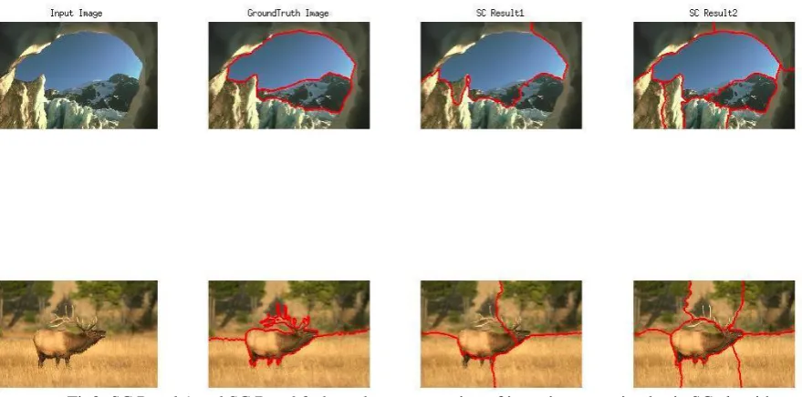
Fig3: SC Result1 and SC Result2 show the segmentation of input images using basic SC algorithm and SC algorithm based on rotation respectively.

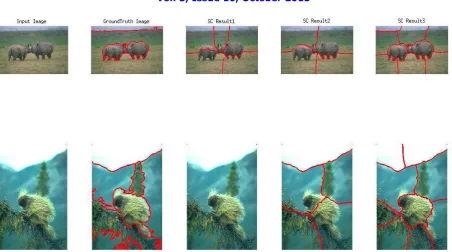
Fig 4: SC Result1, SC Result2 and SC Result3 show the segmentation of input images using basic SC algorithm, SC algorithm based on rotation and improvised SC algorithm based on matrix balancing respectively. The Fig 4 shows the result of proposed algorithm. SC Result1, SC Result2 and SC Result3 are segmented images of 112056 and 347031 using basic SC algorithm, SC algorithm based on rotation and improvised SC algorithm based on rotation respectively. The SC Result1 and SC Result2 show that those methods failed to segment them. But the result of proposed method which is shown as SC Result3 gives better result compared to others.

V. EVALUATIONANDANALYSIS

In this research, evaluation of performance of the algorithms is done using confusion matrix. The Berkeley dataset consists of test images and its corresponding groundtruth image matrices. This groundtruth image matrix contains labels for each pixel which belongs to each segments in the image. The algorithms of existing and developed system also creates matrices of labels of segmented images. Thus using the labeled matrix and its corresponding groundtruth image matrix are used for constructing confusion matrix.

Table 1: Comparison with existing systems

Basic SC Improvised based on

rotation

Matrix balancing

Accuracy 66.292 77.528 81.460

Precision 0.66292 0.7754 0.8148

Recall 0.6510 0.7249 0.8150

Table 1 shows the comparison results of accuracy, precision and recall of the basic SC algorithm, improvised SC algorithm based on rotation and improvised SC algorithm based on matrix balancing respectively. From accuracy comparison table, it is clear that the performance of image segmentation using improvised spectral clustering algorithm based on matrix balancing shows better results.

VI.CONCLUSION

improvised spectral clustering algorithm based on rotation. When Laplacian matrix is balanced, the accuracy of calculation of eigen vector is increased. As a result of this, the performance of data clustering is improved. The algorithms are run on 200 test images of Berkeley Dataset. When local scaling and average alignment criterion for selection of relevant eigen vectors are applied in basic spectral clustering algorithm, the improvised SC based on rotation gives better accuracy than of basic SC algorithm. When matrix balancing is applied to this improvised SC algorithm, the experimental results shows that the proposed method outperforms the other improvised spectral clustering algorithms.

REFERENCES

1. Wang, Yu-Hsiang. Tutorial: Image Segmentation. National Taiwan University, Taipei (2010): 1-36. 2. https://en.wikipedia.org/wiki/Image segmentationApplications

3. Teodorescu, Horia-Nicolai, and Mariana Rusu. Improved Heterogeneous Gaussian and Uniform Mixed Models (GU-MM) and Their Use in Image Segmentation. Romanian Journal of Information Science And Technology 16.1 (2013): 29-51.

4. Aditya Prakash,S Balasubramanian Improvised Eigenvector Selection for Spectral Clustering in Image Segmentation Fourth National Conference on Computer Vision, Pattern Recognition, Image Processing and Graphics (NCVPRIPG), 2013

5. A.Y.Ng, M.Jordan, and Y.Weiss, On spectral clustering: Analysis and an algorithm, Advances in Neural Information Processing Systems, 2002.

6. R.Kannan,S.Vempala and V.Vetta, On Spectral Clustering- Good,Bad,and Spectral Proceedings of the 41st Annual Symposium on Foundations of Computer Science,2000

7. Ulrike von Luxburg , Tutorial on spectral clustering Technical report no.TR-149, 2006

8. Wang Huiqing,Chen Junjie A Semi Supervised Spectral Clustering Algorithm Based on Rough Sets International Conference on Computational Aspects of Social Networks,2010

9. Lihi Zelnik-Manor,Pietro Perona, Self tuning Spectral Clustering, published in Advances in Neural Information Processing Systems, 2004.

10. James, Rodney, Julien Langou, and Bradley R. Lowery. On matrix balancing and eigenvector computation arXiv preprint arXiv:1401.5766 (2014)

11. https://en.wikipedia.org/wiki/Norm %28mathematics% 29 cite note-1

BIOGRAPHY

Deepa Viswam is a M Tech Student in the Department of Computer Science, Government Engineering College Thrissur, Kerala, India. She received B Tech Degree of Computer Science and Engineering in 2011 from Cochin University of Science and Technology, Kochi, Kerala, India. Her research interests are Data mining, Machine learning and Image processing etc.