Game Theoretic Analysis of a Distribution System in Supply Chain

(1)

Abstract

YUAN, PEI-LUN. Game Theoretic Analysis of a Distribution System in

Supply Chain. (Under the direction of Shu-Cherng Fang, and Henry L.

W. Nuttle.)

We consider a distribution system in which one supplier provides a

sin-gle product to several retailers at the beginning of a selling season. The

supplier has inﬁnite capacity. The customer demand at each retailer is

randomly distributed. Customers who encounter a stockout at one

re-tailer may search other rere-tailers for the product. We study the eﬀects

of this market search behavior under both decentralized and centralized

control. For the decentralized control model, we show the necessary and

suﬃcient conditions for the existence of a Nash equilibrium, and the

suf-ﬁcient conditions for its uniqueness. For the centralized control model,

we ﬁnd that the payoﬀ function is submodular, and thus we can only

ob-tain allocations that are locally optimal for the entire supply chain. We

also design a channel coordination mechanism to match the allocations in

the decentralized control model with one of the local optimal allocations

(2)

(3)

Biography

Pei-Lun Yuan was born in Taipei, Taiwan in 1979. She attended the

National Taiwan University through the recommendation of the Taipei

First Girl senior high school in 1997. She graduated with a Bachelor

degree in Chemical Engineering in 2001. She came to North Carolina

State University in the summer of 2001 to begin her graduate studies

in Industrial Engineering. Her main research interests include system

(4)

Acknowledgements

I would like to thank my advisors, Prof. Shu-Cherng Fang and Prof.

Henry L.W. Nuttle. They gave me much encouragement and support to

lead me to my graduate study and research. Thanks for their great

pa-tience and teaching. They take care of students like their children. Under

their instruction, I have learned a lot in these two years.

Our group members, Burcu, Chian-Fen, Hao Cheng, Ilker, Saowanee,

Xi-aoli, Yi Ding, Yi Laio, Yong Wang, and Yue Dai, accompanied and helped

me a lot when I had some doubts in my mind. I am very grateful to Yue

Dai for being so patient in answering my endless questions. She taught

me and gave me much priceless advice.

I have many thanks to my friend, Mark and my families. Especially my

mom, Jing Chen, who is my best listener and always prays for me.

Thanks to God, who tell me to forget the things which are behind and

(5)

List of Figures

1 Decentralized control system . . . 4

2 Centralized control system . . . 5

3 Allocation versus market search probability with 2 retailers . . . 41

4 Proﬁt of retailers versus market search probability with 2 retailers . . 43

5 Proﬁt of supplier versus market search probability with 2 retailers . . 43

6 System proﬁt versus market search probability with 2 retailers . . . . 44

7 Proﬁt improvement after coordination versus market search probability

with 2 retailers . . . 44

8 Wholesale price versus market search probability with 2 retailers . . . 45

9 Allocation versus market search probability with 3 retailers . . . 45

10 Proﬁt of retailers versus market search probability with 3 retailers . . 46

11 Proﬁt of supplier versus market search probability with 3 retailers . . 46

12 System proﬁt versus market search probability with 3 retailers . . . . 47

13 Proﬁt improvement after coordination versus market search probability

with 3 retailers . . . 47

14 Wholesale price versus market search probability with 3 retailers . . . 48

15 Proﬁt percentage after coordination of supplier and retailers versus

(7)

1 Introduction

Capacity allocation plays an important role in supply chain management. Decisions

of both suppliers and retailers are signiﬁcant not only because they determine the

amount of ﬂexibility the supply chain has to meet customers’ demand, but also

be-cause they aﬀect each other. For example, allocating too much capacity to a retailer

results in poor utilization and higher holding cost, but too little capacity results in

poor customer satisfaction and higher penalty cost.

In many supply chains, customers who face a stockout at one retailer may search

for the same product at other retailers. This behavior is called market search.

(Anupindi and Bassok, 1999).

Dai (2002) considers market search in an allocation problem that involves one

supplier and two retailers in the supply chain in a single selling season. Here we

generalize Dai’s (2002) work to the case of one supplier and “multiple” retailers in

the supply chain. We assume the supplier has inﬁnite capacity and the customers’

demand at each retailer is randomly distributed. The market search eﬀect is studied

in two models. In the ﬁrst model, assuming under decentralized control, all retailers

compete with each other. Therefore, “game theory” is applied to decide their

allo-cations. The other model assumes under centralized control, in which all retailers

collaborate with each other. Thus the allocation for the whole supply chain is

opti-mized.

In Chapter 2, some background knowledge and a literature review are given. In

Chapter 3, we introduce the model and notation. In Chapter 4, we obtain the

(8)

In Chapter 5, we show that the payoﬀ function under centralized control is

submod-ular and thus only local optimum allocations can be found. In Chapter 6, we design

a coordination mechanism between decentralized control and centralized control. In

Chapter 7, through numerical experiments, we analyze the eﬀect of coordination and

the market search factor on the retailers, supplier, and whole supply chain. Finally,

(9)

2 Background and Literature Review

In this chapter, we present some important concepts used in this thesis and give a

brief literature review. The concepts include market search, game theory, and channel

coordination. We also introduce a related research issue called product substitution.

2.1 Market search problem

Customers who face a stockout at one retailer may keep on looking for the same

product at other retailers. This phenomenon is called market search and was ﬁrst

introduced by Anupindi and Bassok (1999). They compare the performance of two

systems: one in which the retailers hold stocks separately and the other in which the

retailers centralize stocks at a single location. They ﬁnd that whether centralization

of stocks by retailers increases proﬁts for the manufacturer depends on the level of

market search in the supply chain. The level of market search is measured as the

fraction of customers who transfer their demand from the original retailer they visit

to other retailers when they encounter a stockout. They show that there exists a

threshold of market search level beyond which the system proﬁt may decrease with

centralization of stocks.

In Anupindi and Bassok’s (1999) model, centralization means that all stocks in

the supply chain are located at one retailer. But in our work, centralization means

collaboration and information sharing. The inventory is held at diﬀerent retailers

based on the customer demand.

With customers’ market search behavior, we analyze the diﬀerences between two

(10)

Supplier

Retailer 1

Retailer 2

Retailer i

Retailer j

Retailer n

yn y1

y2

yi

yj

Retailer i

Retailer j

Customers Demand Di

Customers Demand D_j

Stockout, penalty cost required Demand

from i to j, aij

Demand from j to i, aji Stockout, penalty cost required

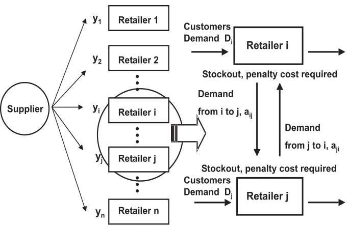
Figure 1: Decentralized control system

(Figure 2). Under decentralized control, each retailer makes its order decision by itself

and does not cooperate with other retailers. To maximize its own proﬁt, each retailer

has to determine its order strategy so as to compete with other retailers. Under

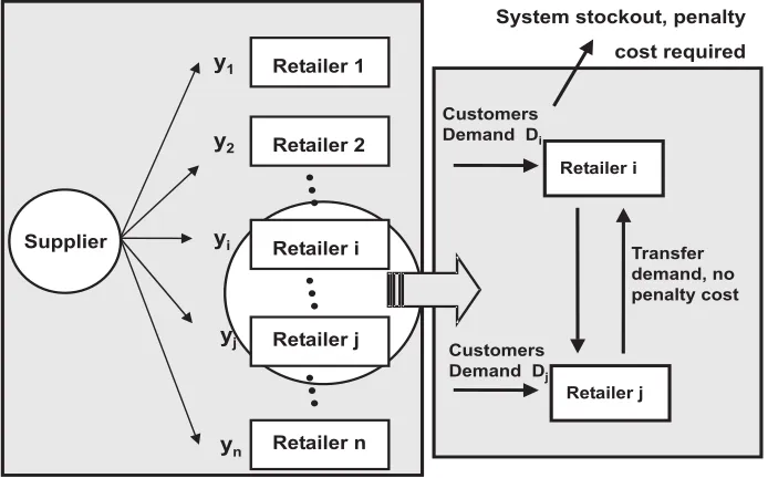
cen-tralized control, all retailers in the supply chain are willing to cooperate and make

the allocation decisions together with the supplier. If customers encounter a stockout

at one retailer and they want to look for the same product at other retailers, the

initial retailer may tell the customers at which retailers this product is still available.

Therefore, the whole supply chain will pay less penalty cost for lost customers.

2.2 Game theory

Decentralized control is often used in supply chains. Since the ordering decision of

(11)

Supplier

Retailer 1

Retailer 2

Retailer i

Retailer j

Retailer n

yn y1

y2

yi

yj

Retailer i Customers

Demand D_i

Customers Demand D_j

Transfer demand, no penalty cost

Retailer j

System stockout, penalty cost required

Figure 2: Centralized control system

trying to maximize their own proﬁts. A strategic interaction results from retailers’

ordering decisions. Therefore, we apply game theory to analyze the allocation

deci-sions of retailers in a decentralized control system.

Game theoryhas been widely used in supply chain management (Mesterton, 2000).

The term “players” refers to the diﬀerent parties who compete with each other in the

supply chain. “Payoﬀ function” is the proﬁt function or utility function of each

player. A strategic game is a model of interactive decision-making in which each

player chooses his or her strategy once and for all, and these choices are made

simu-taneously. In a strategic game, the number of players has to be ﬁnite. In game theory,

the players are assumed to be rational. They always try to maximize their individual

proﬁt. The so-calledNash equilibrium establishes when no player has an action

(12)

given that every other player chooses his/her equilibrium action, i.e., no player can

proﬁtably deviate when we give other players’ strategies (Osborne, 1996).

Game theory has been applied to solve some inventory problems. Parlar (1988)

studies the substitutable product problem as an extension of the classical newsvendor

problem. In his two-player model, product substitution (which we will describe in

detail later) occurs with a certain probability when customers encounter a stockout.

For this problem, he proves the existence of a unique Nash equilibrium. Lippman and

McCardle (1994) also study an extension of the classical newsvendor problem. They

assume the salvage value of excess inventory and penalty for unsatisﬁed demand are

zero. Under these assumptions, they examine the equilibrium of inventory levels and

rules for reallocating excess demand. They also provide existence conditions for a

Nash equilibrium when two or more newsvendors are involved.

Under decentralized control, the retailers are the players, and their individual

proﬁt functions are the payoﬀ functions. We apply game theory to analyze the best

strategies for retailers to order the inventory they need. Game theory is also used to

determine the existence conditions of a Nash equilibrium for the decentralized model

in Chapter 4. Futhermore, when a Nash equilibrium exists, we also want to know the

conditions which support global stability of the solution.

2.3 Channel coordination

Compared to decentralized control, centralized control yields more proﬁt for the

sup-ply chain as a whole. However, in reality, most retailers will not cooperate, share

(13)

sup-plier unless they are owned by the same company. To improve the performance under

decentralized control, coordination mechanisms can be designed by altering the

indi-vidual payoﬀ functions. In this way, it may be possible to reach the same solution and

the overall proﬁt as with a centralized control system. This approach is called

chan-nel coordination. In a supply chain, channel coordination can be achieved through

a contract between the supplier and retailers. This contract indicates beneﬁt

shar-ing among the supplier and retailers after coordination. To understand the eﬀect of

coordination between supplier and retailers in our senario, we will analyze the proﬁt

ratio of supplier and retailers after channel coordination.

2.4 Product substitution problem

In addition to searching for the same product at other retailers, customers may also

substitute an out-of-stock product with diﬀerent products. This is calledproduct

sub-stitution. Compared to the market search problem, product substitution problem is

more general. McGillivray and Silver (1978) consider the substitution of two identical

products with independent normally distributed demands and develop heuristics to

obtain the optimal stocking level. Palar and Goyal (1984) analyzed this problem of

two substitutable products with stochastic demands. Pasternak and Drezner (1991)

provide an analytical solution to the problem of two substitutable products and

con-clude that substitution gives a lower revenue. Many people have followed this stream

to work on similar problems. However, it is very diﬃcult to deal with problems which

have more than three substitutable products using the Leibnitz formula. In a 2001

paper, Rudi provides a more tractable expression for derivatives of high dimensional

integrals. Netessine (2001) adopts Rudi’s expression to solve more complex cases of

(14)

(15)

3 The model and basic notation

Consider one supplier distributing one product to _n retailers who sell this product to

customers in a single period on season. If customers who visit retailer _i at begining

face a stockout, some of them may search for the same product at a second retailer

j with probability _a_ij. We assume that customers at most visit two retailers, i.e., if

they encounter a stockout at the second visited retailer, they will not search anymore.

Since customers may transfer their demand between retailers, the total customer

demand at any retailer can be separated into local demand anddistant demand. Local

demand is from the customers who visit this retailer at ﬁrst, whiledistant demand is

the demand transferred from other stocked out retailers. The total customer demand

is called eﬀective demand. Usually, retailers will give priority to their local demand

and use the remaining inventory, if any, to satisfy their distant demand. The

inven-tory of each retailer certainly aﬀects other retailers’ distant demand.

We assume that the supplier has inﬁnite capacity to provide the product. At the

beginning of the season, retailers will receive whatever amount of product that they

ordered. At the end of the season, a holding cost or stockout penalty is incurred by

each retailer depending on whether there is unsold stock or a stockout. In the

decen-tralized control model, the stockout penalty cost is modeled as incurred for unsatisﬁed

local demand. In the centralized control model, the supplier and all retailers can be

viewed as a whole. Therefore, the average penalty cost of all retailers is incurred by

the system when customers leave the supply chain without a purchase.

In the decentralized control model, each retailer is assumed to be an independent

(16)

market search probability of customers. The problem of making optimum ordering

decisions by the retailers is modeled as a game.

In the centralized control model, since the supplier and all retailers cooperate with

each other, instead of playing a game, they have to decide the total production and

allocations together so as to maximize the total expected proﬁts of the supply chain.

Following is the notation that we use in the two models:

for the supplier:

K: the capacity of the supplier;

c: the unit production cost;

wi: the wholesale price to retailer i, i= 1, ..., n;

for retailer _{i, i}= 1_{, ..., n}:

si: the unit selling price for local demand;

ti: the unit selling price for distant demand;

hi: the unit holding cost per unit of product left at the end of the season;

pi: the per unit stockout penalty cost;

¯

p: the average unit stockout penalty cost for the_n retailers;

Di: a continuous random variable, denoting a stochastic local demand;

(17)

Fi(Di): the cumulative distribution function ofDi;

aij: the market search probability from retailer ito retailer j, an element of the

market search matrix, 0 ≤_a_ij ≤1,_a_ii = 0;

yi: the allocation, i.e., inventory, at the beginning of the season;

Ri: the eﬀective demand. It is the summation of local demand and distant

demand,

Ri =Di+ n

j=1aji

(_y_j −_D_j)−_, (1)

where (_x)−= max{−x,0}, and (_x)+= max{x,0};

πi(y1, y2, ..., yn): the expected payoﬀ given all retailers’ allocations,y1,y2,...,yn.

Following Pasternack and Drezner (1991), we make the following assumptions:

(A1) _s_i _{> w}_i _>0_{, i}= 1_{, ..., n};

(A2) _t_i _{> w}_i _>0_{, i}= 1_{, ..., n};

(A3) _s_i _{> t}_i−_p_i_{, i}= 1_{, ..., n};

Assumptions (A1) and (A2) express the idea that the product selling price should

be higher than its cost. Assumptions (A3), as observed by Pasternack and Drezner,

describes the phenomenon that the retailers will satisfy the local demand at ﬁrst, and

then use the remaining inventory, if any, to satisfy a distant demand. Assumption

(18)

only one unit of product left and faces both local and distant demand simultaneously.

Because the local selling price is higher than the distant selling price less the shortage

penalty, retailers will consider local customers as their priority.

If retailer_icannot distinguish the local demand from distant demand, i.e.,_s_i =_t_i,

then assumption (A3) for retailer _i is unnecessary. However, for other retailers who

can tell the diﬀerence between local customers and distant ones, they still need

(19)

4 Decentralized Control System

Under decentralized control, each retailer makes his/her own order decision, and does

not cooperate with other retailers. To maximize his/her own proﬁt, each retailer

has to manage his/her order strategy in competition with other retailers. Here we

assume the supplier has inﬁnite capacity, i.e. all retailers can order and be allocated

the amount of inventory they need. Given that retailer _i’s order is _y_i, the payoﬀ for

retailer _i consists of:

(i) Purchasing cost: _w_i_y_i;

(ii) Holding cost: _h_i(_y_i−_R_i)+;

(iii) Penalty cost: _p_i(_y_i−_D_i)−;

(iv) Selling revenue: _s_imin{y_i_{, D}_i}+_t_imin{(_y_i−_D_i)+_,n_j₌₁_a_ji(_y_j −_D_j)−}.

Thus retailer _i’s expected payoﬀ function is

πi(y1, y2, . . . , yn) = E[simin{yi, Di}+timin{(yi−Di)+, n

j=1

aji(yj −Dj)−}

−wiyi

−hi(yi−Ri)+ −pi(yi−Di)−]

= _E[_s_i_y_i−_w_i_y_i+_p_i(_y_i−_D_i)

−hi(yi−Ri)+

−(_s_i+_p_i−_t_i)(_y_i−_D_i)+

−ti[(yi−Di)+− n

j=1

(20)

where min{a, b}=_a−(_a−_b)+.

Lemma 1 Given _y_j_{, j} = 1_{, . . . , n, j} =_{i, π}_i(_y₁_{, . . . , y}_n) is strictly concave in _y_i.

Proof The ﬁrst derivative of _π_i(_y₁_{, . . . , y}_n) with respect to _y_i is

∂πi(y1, y2, . . . , yn)

∂yi = (si−wi+pi) −∂E[hi(yi−Ri)+]

∂yi

−∂E[(si+pi−ti)(yi−Di)+] ∂yi

−∂E[ti((yi−Di)+−

_n

j=1aji(yj −Dj)−)+]

∂yi (3)

= (_s_i−_w_i+_p_i)

−(_s_i+_p_i−_t_i)_{P r}(_y_i _{> D}_i)

−(_h_i+_t_i)_{P r}(_y_i _{> R}_i)_. (4)

As noted in Netessine (2001), due to the necessity of dealing with nested integrals

of high dimensionality over the regions formed by intersections of a large number of

hyperplanes, it is very diﬃcult to take derivatives by the Leibnitz formula. Thus to

go from (3) to (4), we directly utilize the deﬁnition as in Rudi (2001).

The derivate of the function _f(_x) with respect to variable _x is deﬁned as follows,

∂f(_x)

∂x = lim→0

f(_x+)−_f(_x)

(21)

First, we work with the second term of (3) and determine the derivative of

E[_h_i(_y_i−_R_i)+]

∂E[_h_i(_y_i−_R_i)+]

∂yi = hi lim→0E

(_y_i+−_R_i)+−(_y_i−_R_i)+

.

We distinguish these cases, namely

(_y_i+−_R_i)+−(_y_i−_R_i)+ =

        

0 if _y_i−_R_i ≤ −;

(_y_i+−_R_i) if− < y_i−_R_i ≤0;

if 0_{< y}_i−_R_i_.

Suppose_>0 (analogously, for_<0), taking the derivative for each of the three

cases, we obtain,

∂E[_h_i(_y_i−_R_i)+]

∂yi

=_h_ilim

→0

0_{P r}(_y_i−_R_i _<−) + _yyi+

i (yi+−x)fRi(x)dx+P r(yi > Ri)

. (5)

(22)

hilim_→0 yi+

yi (yi+−x)fRi(x)dx

= _h_ilim

→0

E[_y_i+−_R_i|y_ii_{< y}_i+]

P r(yi ≤ Ri < yi + ).

Obviously,

lim

→0

E[_y_i+−_R_i|y_i ≤_R_i _{< y}_i+]

< 1.

Therefore,

lim

→0

yi+

yi (yi+−x)fRi(x)dx

= 0.

Consequently,

∂E[_h_i(_y_i−_R_i)+]

(23)

The third term of (3) is taken from the derivative of_E[(_s_i+_p_i−_t_i)(_y_i−_D_i)+] in

the same way. Hence

∂E[(_s_i+_p_i−_t_i)(_y_i−_D_i)+]

∂yi

= (_s_i+_p_i −_t_i)_{P r}(_y_i_{> D}_i)_. (7)

We determine the derivative of the fourth term of (3):

∂E[_t_i((_y_i−_D_i)+−_jn₌₁_a_ji(_y_j −_D_j)−)+]

∂yi = tilim→0E

((_y_i+−_D_i)+

− n

j=1

aji(yj −Dj)−)+−((yi−Di)+

− n

j=1

aji(yj −Dj)−)+

.

Here we have four cases, for the numerator of the expression under the expectation,

namely

((_y_i+−_D_i)+−

n

j=1

aji(yj −Dj)−)+−((yi−Di)+− n

j=1

aji(yj −Dj)−)+

=                                 

if _y_i−_D_i _>0_,

and (_y_i−_D_i)+−n_j₌₁_a_ji(_y_j −_D_j)−_>0;

yi+−Di if − < yi−Di ≤0,

yi+−Di−nj=1aji(yj−Dj)− if − < yi−Di ≤0,

and − <(_y_i−_D_i)+−_jn₌₁_a_ji(_y_j −_D_j)−≤0;

(24)

This leads to

∂E[_t_i((_y_i−_D_i)+−_jn₌₁_a_ji(_y_j −_D_j)−)+]

∂yi = tilim→0

P r(_y_i−_D_i _>0_,

(_y_i−_D_i)+−

n

j=1

aji(yj−Dj)−>0)

+

_y_i₊

yi

(_y_i+−_x)_f_D_i(_x)_dx

+

_y_i₊

yi

(_y_i+−_x

−n j=1

aji(yj−Dj)−)fDi(x)dx

+0_{P r}(_y_i−_D_i ≤ −)

.

(8)

As described before, the second term of (8) can be re-written as

lim

→0

yi+

yi (yi+−x)fDi(x)dx

= lim

→0

E[_y_i+−_D_i|y_i ≤_D_i _{< y}_i+]

P r(yi ≤ Di < yi + ).

(25)

lim

→0

E[_y_i+−_D_i|y_i ≤_D_i_{< y}_i+]

< 1.

Hence,

lim

→0

yi+

yi (yi+−x)fDi(x)dx

= 0.

Also, the third term of (8) can be re-written as

lim

→0

yi+

yi (yi+−x−

_n

j=1aji(yj−Dj)−)fDi(x)dx

= lim

→0

E[_y_i+−_D_i−n_j₌₁_a_ji(_y_j−_D_j)−|y_i ≤_D_i _{< y}_i+]

P r(yi ≤Di < yi+)

where

lim

→0

E[_y_i+−_D_i−n_j₌₁_a_ji(_y_j−_D_j)−|y_i ≤_D_i _{< y}_i+]

< 1.

Consequently,

lim

→0

yi+

yi (yi+−x−

_n

j=1aji(yj−Dj)−)fDi(x)dx

(26)

Thus, equation (8) can be re-written as

∂E[_t_i((_y_i−_D_i)+−_jn₌₁_a_ji(_y_j−_D_j)−)+]

∂yi = tiP r(yi−Di >0,

(_y_i−_D_i)+−

n

j=1

aji(yj −Dj)−>0),

= _t_i_{P r}(_y_i−_R_i _>0)_. (9)

From (6), (7), and (9), we can obtain the following result:

∂πi(y1, y2, . . . , yn)

∂yi = [si−wi+pi] −hiP r(yi > Ri)

−(_s_i+_p_i−_t_i)_{P r}(_y_i_{> D}_i)

−tiP r(yi > Ri)

= [_s_i−_w_i+_p_i]

−(_s_i+_p_i−_t_i)_{P r}(_y_i_{> D}_i)

−(_h_i+_t_i)_{P r}(_y_i_{> R}_i)

= [_s_i−_w_i+_p_i]

−(_s_i+_p_i−_t_i)_F_D_i(_y_i)

−(_h_i+_t_i)_F_R_i(_y_i) (10)

Taking the derivative of (10) with respect to _y_i, we obtain the second derivative

(27)

∂2πi

∂2yi = (−si−pi+ti)fDi(yi) −(_t_i+_h_i)_f_R_i(_y_i)

By assumptions (A2) and (A3), we know that_t_i _>0 and_s_i+_p_i _{> ti},thus ∂2πi

∂2_y_i <0.

Since the second derivative of _π_i(_y₁_{, . . . , y}_n) with respect to _y_i is less than zero,

(28)

Lemma 2 If each player’s payoﬀ function _π_i(_y₁_{, . . . , y}_n) is continuous in all decision

variables (_y₁_{, . . . , y}_n) and concave in its own decision variable _y_i, then the game has

at least one Nash equilibrium which is determined by letting the ﬁrst partial derivative

of each player’s payoﬀ function with respect to its own decision variable be zero.

Proof The deﬁnition of a noncooperative _n-person convex game is given below by M. Dresher and S. Karlin (1953):

(i) The_ith player’s strategy space is a compact convex set_X_i of a topological linear

space _E_i;

(ii) The _ith player’s payoﬀ_π_i(_x₁_,· · · _{, x}_i_,· · · _{, x}_n) is concave with respect to his own

strategy variable _x_i ∈_X_i;

(iii) The sum of payoﬀs n_i₌₁_π_i(_x₁_,· · ·_{, x}_i_,· · · _{, x}_n)is continuous over the cartesian

product space _X₁⊗_X₂⊗ · · · ⊗_X_n;

(iv) For each ﬁxed _x_i_{, π}_i(_x₁_,· · · _{, x}_i₋₁_{, x}_i_{, x}_i₊₁_,· · · _{, x}_n) is a continuous function of

the (_n-1)-tuple [_x₁_,· · · _{, x}_i₋₁_{, x}_i₊₁_,· · · _{, x}_n]∈_X₁⊗ · · · ⊗_X_i₋₁⊗_X_i₊₁⊗ · · · ⊗_X_n

respectively.

From Theorem 3.1 of Nikaido and Isora (1955), we know that a convex game

al-ways has at least one Nash equilibrium solution. Since the noncooperative game in

our decentralized control model satisﬁes the conditions of a_n-person convex game, it

has at least one Nash equilibrium.

According to Moulin (1986), to compute all Nash equilibra of a given game, G,

we need to solve the system:

Π_i(_y∗) = max

yi Πi(yi, y

∗

(29)

where_i= 1_{, . . . , n}, and_y₋∗_i is the vector of what strategies of the players other than_i.

Equation (11) says that given all the other player’s strategies, the Nash equilibrium

strategy for player_i is the one that maximizes his or her proﬁt. If Π_i is concave in_y_i,

and Π_i is diﬀeretiable in_y_i, the above system is equivalent to the ﬁrst order conditions

∂Π_i

∂yi(y

∗_{) = 0}_,

where_i= 1_{, . . . , n}.

From Lemma 1 and Lemma 2, we can conclude the following theorem.

Theorem 3 There exists at least one Nash equilibrium for our decentralized control model which may be obtained by solving the system of equations that results from

setting the ﬁrst partial derivative of each player’s payoﬀ function with respect to its

own decision variable to be zero.

Basically, at least one Nash equilibrium can be found in the decentralized control

system by solving the ﬁrst order conditions. We would also like to know the

unique-ness conditions of aNash equilibrium in the decentralized control system.

Theorem 3 of Chapter 6 of Moulin (1984) states that if the payoﬀ function is twice

diﬀerentiable in all of its variables with

∂2πi ∂y2i <

(30)

The system is globally stable with a unique Nash equilibrium if

|∂2πi ∂y_i2| >

j,j=i |∂2πi

∂yiyj|,

for all _{i, j} = 1_{, . . . , n, j} =_i. (12)

In other words, there exists a unique Nash equilibrium for the decentralized

con-trol model if its payoﬀ function satisﬁes the inequalities of (12).

According to Dai (2002), when there are only two retailers in the supply chian,

we can ﬁnd the necessary and suﬃcient conditions for the existence of a unique Nash

equilibrium. When we have more than two retailers, there only exists some suﬃcient

conditions for a unique Nash equilibrium.

Theorem 4 If n_j₌₁_a_ji _< 1, for all _i and _{j, j} = _i, the Nash equilibrium of the decentralized control model is unique.

Proof From assumption (A3), we know that _s_i+_p_i−_t_i _>0. Since n_j₌₁_a_ji _<1 for all _i, and _{j, j} =_i,

fRi(yi)>

j,j=i

(_a_ji_f_R_i_|_D_j_≥_y_j(_y_i)_{P r}(_D_j ≥_y_j))_.

Consequently,

| −(_s_i +_p_i−_ti)_f_D_i(_y_i)−(_t_i+_h_i)_f_R_i(_y_i)|_>

j,j=i

(31)

where _{i, j} = 1_{, . . . , n}, and_i=_j.

Equivalently, we have

|∂2πi ∂y2_i |>

j,j=i | ∂2πi

∂yiyj|, wherei, j = 1, . . . , n, j =i

Therefore, n_j₌₁_a_ji _< 1, for all _i and _{j, j} = _i, is a suﬃcient condition to quarantee

(32)

5 Centralized Control System

In the centralized control model, we assume that all retailers in the supply chain

are willing to cooperate and make the allocation decisions together with the supplier

because this approach will maximize the expected total proﬁt of the whole supply

chain. Since all retailers cooperate with each other in the supply chain, when

cus-tomers encounter a stockout at one retailer and decide to look for the product at

other retailers, the initial retailer may tell the customers at which other retailers they

may ﬁnd the product. We assume that a customer may visit up to two retailers in

search of the product before leaving the system. The stockout penalty is incurred

only when a customer leaves the system without purchasing the product. Because

the supplier and retailers can be viewed as a whole system, we assume that the unit

penalty cost for losing a customer to be the average of the unit penalty costs for

individual retailers in the decentralized model.

We assume the supplier has inﬁnite capacity, and_y_i is the order (and allocation)

for retailer _i. The payoﬀ function for the whole supply chain consists of:

(i) Production cost: _cK =_c(_y₁+_{. . .}+_y_n) = _cn_i₌₁_y_i;

(ii) Holding cost: n_i₌₁_h_i(_y_i−_R_i)+;

(iii) Penalty cost:

_n

i=1p¯[(yi−Di)−(1−

_n

j=1aij) + (

_n

j=1aji(yj−Dj)−−(yi−Di)+)+]

=n_i₌₁_p¯[(_y_i−D_i)−(1−n_j₌₁_a_ij)+n_j₌₁_a_ji(_y_j−D_j)−−(_y_i−D_i)++(n_j₌₁_a_ji(_y_j−

Dj)−−(yi−Di)+)−];

(33)

_n

i=1[simin{yi, Di}+timin{(yi−Di)+,

_n

j=1aji(yj−Dj)−}]

=n_i₌₁[_s_i_y_i−_s_i(_y_i−_D_i)++_t_i(_y_i−_D_i)+−_t_i[(_y_i−_D_i)+−n_j₌₁_a_ji(_y_j−_D_j)−]+]_.

Thus the expected payoﬀ function of the whole supply chain is

π(_y₁_{, y}₂_{, . . . , y}_n) = _E[

n

i=1

(_s_i_y_i−_s_i(_y_i−_D_i)++_t_i(_y_i−_D_i)+

−ti((yi−Di)+− n

j=1

aji(yj−Dj)−)+)

−c n

i=1

yi

−n i=1

hi(yi−Di− n

j=1

aji(yj −Dj)−)+)

−_p¯

n

i=1

((_y_i−_D_i)−(1−

n

j=1

aij))

−_p¯

n i=1 ( n j=1

aji(yj−Dj)−−(yi−Di)+)

−_p¯

n i=1 ( n j=1

aji(yj−Dj)−−(yi−Di)+)−]

= _E[

n

i=1

(_s_i−_c+ ¯_p)_y_i

− n

i=1

(_s_i−_t_i)(_y_i−_D_i)+

− n

i=1

(_t_i+ ¯_p)((_y_i−_D_i)+−

n

j=1

aji(yj−Dj)−)+

− n

i=1

hi(yi−Di− n

j=1

aji(yj −Dj)−)+]. (13)

(34)

product” problem is submodular. In our market search problem, since the product

sold by diﬀerent retailers is the same, they are substitutable. In Lemma 5, we show

that the payoﬀ function is submodular.

Lemma 5 In the centralized control model, the payoﬀ function _π(_y₁_{, y}₂_{, . . . , y}_n) is

submodular in _y₁_{, y}₂_{, . . . , y}_n.

Proof To show the payoﬀ function _π(_y₁_{, y}₂_{, . . . , y}_n) is submodular in _y₁_{, y}₂_{, . . . , y}_n, we refer to Sundaram (1999). It is suﬃcient to demonstrate that the second order

cross-partial derivatives are non-positive.

The ﬁrst derivative of_π(_y₁_{, y}₂_{, . . . , y}_n) with respect to _y_i is

∂π(_y₁_{, y}₂_{, . . . , y}_n)

∂yi

= (_s_i−_c+ ¯_p)

−∂E[

_n

i=1(si−ti)(yi−Di)+] ∂yi

−∂E[

_n

i=1(ti+ ¯p)((yi−Di)+−nj=1aji(yj −Dj)−)+] ∂yi

−∂E[

_n

i=1hi(yi−Di−

_n

j=1aji(yj −Dj)−)+]

∂yi (14)

= (_s_i−_c+ ¯_p)

−(_s_i−_t_i)_{P r}(_y_i _{> D}_i)

−(_t_i+_h_i+ ¯_p)_{P r}(_y_i _{> R}_i)

− n

j=1,j=i

(_t_j+_h_j+ ¯_p)_a_ij_{P r}(_D_i_{> y}_i_{, R}_j _{< y}_j)_. (15)

For (14) and (15), it is easy to see the equivalence of the ﬁrst two terms in (14)

(35)

given as follows.

First, we can separate the third term of (14) into two parts.

∂E[n_i₌₁(_t_i+ ¯_p)((_y_i−_D_i)+−n_j₌₁_a_ji(_y_j−_D_j)−)+]

∂yi

= lim

→0

(_t_i+ ¯_p)((_y_i+−_D_i)+−

n

j=1

−(_t_i+ ¯_p)((_y_i−_D_i)+−

n

j=1

aji(yj −Dj)−)+

+ lim →0 n

j=1,j=i

(_t_j + ¯_p)((_y_j−_D_j)+−

n

i=1

aij(yi+−Di)−)+

−(_t_j + ¯_p)((_y_j −_D_j)+−

n

i=1

aij(yi−Di)−)+

. (16)

With (_t_i + ¯_p) being factored out, the numerator of the ﬁrst term in (16) can be

expressed as:

((_y_i+−_D_i)+−

n

j=1

aji(yj−Dj)−)+−(ti + ¯p)((yi−Di)+− n

j=1

aji(yj −Dj)−)+

=                                 

if _y_i−_D_i _>0_,

yi+−Di if − < yi−Di ≤0,

yi+−Di−nj=1aji(yj−Dj)− if − < yi−Di ≤0,

and − <(_y_i−_D_i)+−_jn₌₁_a_ji(_y_j −_D_j)−≤0;

(36)

After taking the derivative for the four cases, the ﬁrst term of (16) can be

re-written as:

lim

→0

(_t_i+ ¯_p)((_y_i+−_D_i)+−

n

j=1

−(_t_i+ ¯_p)((_y_i−_D_i)+−

n

j=1

aji(yj −Dj)−)+

= (_t_i+ ¯_p) lim

→0

P r(_y_i−_D_i _>0_,(_y_i−_D_i)+−

n

j=1

aji(yj−Dj)− >0)

+

_y_i₊

yi

(_y_i+−_x)_f_D_i(_x)_dx

+

_y_i₊

yi

(_y_i+−_x−

n

j=1

aji(yj −Dj)−)fDi(x)dx

+0_{P r}(_y_i−_D_i ≤ −)

, (17)

= (_t_i+ ¯_p)_{P r}(_y_i−_D_i _>0_,(_y_i−_D_i)+−

n

j=1

aji(yj −Dj)− >0),

= (_t_i+ ¯_p)_{P r}(_y_i_{> R}_i)_.

With (_t_j+ ¯_p) factored out, the numerator of the second term of (16) can be expressed

as

((_y_j−_D_j)+−

n

i=1

aij(yi+−Di)−)+−(tj + ¯p)((yj−Dj)+− n

i=1

(37)

=                           

−aij if yi−Di <−,

and (_y_j −_D_j)+−n_i₌₁_a_ij(_y_i−_D_i)− _>0;

−aij(yi+−Di) if −≤yi−Di <0,

and (_y_j −_D_j)+−n_i₌₁_a_ij(_y_i−_D_i)− _>0;

0 if 0≤_y_i−_D_i_,

and 0≤ (_y_j−_D_j)+−_in₌₁_a_ij(_y_i−_D_i)−_.

Then we take the derivative for these three cases,

lim

→0

n

j=1,j=i

(_t_j + ¯_p)((_y_j−_D_j)+−

n

i=1

aij(yi+−Di)−)+

−(_t_j+ ¯_p)((_y_j−_D_j)+−

n

i=1

aij(yi−Di)−)+

= (_t_j + ¯_p) lim

→0

n

j=1,j=i

−aijP r(yi−Di <−,(yj−Dj)+− n

i=1

aij(yi−Di)−>0)

−

_y_i₊

yi

aij(yi+−x)fDi(x)dx

+0_{P r}(0≤_y_i−_D_i_,0≤(_y_j −_D_j)+−

n

i=1

aij(yi−Di)−)

=

n

j=1,j=i

(_t_j+ ¯_p)_{P r}(_y_i−_D_i _<0_,(_y_j−_D_j)+−

n

i=1

aij(yi−Di)− >0)

=

n

j=1,j=i

(38)

Similarly, for the fourth term of (14), we can show that

∂E[n_i₌₁_h_i(_y_i−_D_i−n_j₌₁_a_ji(_y_j−_D_j)−)+]

∂yi = hiP r(yi> Ri)

+

n

j=1,j=i

hjaijP r(Di > yi, Rj < yj)

(19)

From equations (16) to (19), we obtain the ﬁrst derivative of the payoﬀ function

with respect to _y_i in centralized control system as (15).

Taking the derivative of (15), we obtain the second derivative of_π(_y₁_{, . . . , y}_n) with

respect to _y_i as

∂2π

∂2yi = −(si−ti)fDi(yi) −(_t_i+_h_i+ ¯_p)_f_R_i(_y_i)

− n

j=1,j=i

(_t_j+_h_j + ¯_p)_a2_ij_f_R_j_|_D_i_>y_i(_y_j)_{P r}(_D_i _{> y}_i)_. (20)

The ﬁrst two terms of (20) are easily seen to follow from (15). The third term of

(20) requires some explanation.

∂P r(_D_i _{> y}_i_{, R}_j _{< y}_j)

∂yi = lim→0

P r(_D_i _{> y}_i+_{, D}_j +_a_ij(_y_i+−_D_i)− _{< y}_j)

−P r(_D_i _{> y}_i_{, D}_j+_a_ij(_y_i−_D_i)−_{< y}_j)

(39)

Then we can split up the numerator into three cases:

P r(_D_i _{> y}_i+_{, D}_j +_a_ij(_y_i+−_D_i)− _{< y}_j)−_{P r}(_D_i _{> y}_i_{, D}_j+_a_ij(_y_i−_D_i)− _{< y}_j)

=

              

P r(_D_i _{> y}_i+_{, D}_j −_a_ij(_y_i+−_D_i)_{< y}_j)

−P r(_D_i _{> y}_i_{, D}_j −_a_ij(_y_i−_D_i)_{< y}_j) if _D_i−_y_i _{> ,}

−P r(_D_i _{> y}_i_{, D}_j −_a_ij(_y_i−_D_i)_{< y}_j) if 0_{< D}_i−_y_i ≤_,

0 if _D_i−_y_i ≤0_.

Therefore,

∂P r(_D_i _{> y}_i_{, R}_j _{< y}_j)

∂yi = lim→0

(_{P r}(_D_i_{> y}_i+_{, D}_j−_a_ij(_y_i+−_D_i)_{< y}_j)

−P r(_D_i _{> y}_i_{, D}_j −_a_ij(_y_i−_D_i)_{< y}_j))_{P r}(_D_i−_y_i _>)

−(_{P r}(_D_i_{> y}_i_{, D}_j −_a_ij(_y_i−_D_i)_{< y}_j))_{P r}(0_{< D}_i−_y_i ≤)

.

= _a_ij_f_R_i_|_D_i_>y_i(_y_j)_{P r}(_D_i _{> y}_i)

In a similar manner, we can show that the second order cross-partial derivative of

(40)

∂2π

∂yiyj = −(ti+hi+ ¯p)ajifRi|Dj>yj(yi)P r(Dj > yj) −(_t_j+_h_j + ¯_p)_a_ij_f_R_j_|_D_i_>y_i(_y_j)_{P r}(_D_i _{> y}_i)

− n

r=1,r=i,j

(_t_r+_h_r+ ¯_p)_a_ir_a_jr_f_R_r_|_D_i_>y_i_,D_j_>y_j(_y_r)_{P r}(_D_i_{> y}_i_{, D}_j _{> y}_j)_.

Following assumption (A2), since the unit selling price for distant demand is

al-ways greater than zero, the second order cross-partial derivative of _π(_y₁_{, . . . , y}_n) with

respect to_y_i_{, y}_j is less than zero. Thus_π(_y₁_{, y}₂_{, . . . , y}_n) is submodular in_y₁_{, y}₂_{, . . . , y}_n_.

Because the payoﬀ function in the centralized control model is only submodular

and not concave, a solution of the ﬁrst order conditions does not guarantee global

(41)

6 Channel Coordination

In reality, retailers usually do not cooperate, share their information, and manage

their inventory allocations in concert with the supplier for the advantage of the whole

system unless they are owned by the same company. However, through channel

co-ordination, the supply chain operating under decentralized control still can reach the

same solution and overall proﬁt as under centralized control.

To accomplish channel coordination, there are three steps commonly used in

sup-ply chain inventory management research. First, apsup-ply game theory to the system

under decentralized control and ﬁnd the Nash equilibrium satisfying the ﬁrst order

conditions. Next, determine the optimal inventory allocation under centralized

con-trol. Third, if the solution under centralized control is better than the solution under

decentralized control, alter the players’ payoﬀs.

In the third step, in order to alter the players’ payoﬀs, we have to ﬁnd a parameter

that only exists in the payoﬀ function of the decentralized control model. Thus we

maintain the optimal solution of the centralized control model, and adjust the payoﬀ

of the decentralized control model to yield the same solution. Because the

“whole-sale price” aﬀects the Nash equilibrium in the decentralized control model, but has

no eﬀect on solutions to the centralized control model, we may utilize the wholesale

price _w_i to provide the coordination between the two solutions.

For the decentralized control model, we know that the Nash equilibrium can be

easily found from the ﬁrst order conditions. Similarly, we can ﬁnd a local optimal

so-lution for the centralized control model. If we can ﬁnd a better local optimal soso-lution

(42)

the same solution under decentralized control. The coordination is achieved by solving

∂πi ∂yi =

∂π

∂yi, where i= 1, . . . , n.

Then the wholesale price can be determined by

wi = c+pi−p¯

−piP r(yi > Di)

+¯_{pP r}(_y_i_{> R}_i)

+

n

j=1,j=i

(_t_j+_h_j + ¯_p)_a_ij_{P r}(_D_i _{> y}_i_{, R}_j _{< y}_j)_, where _i= 1_{, . . . , n}. (21)

to achieve channel coordination between the system under centralized control and

under decentralized control. But the wholesale prices have to satisfy the assumptions

(A1) _s_i _{> w}_i _>0 and (A2) _t_i _{> w}_i _>0, for_i= 1_{, ..., n}.

According to the paper, “Vendor Managed Inventories and Supply Chain

Coordi-nation :The Case with One Supplier and Competing Retailers” by Bernstein, Chen ,

and Federgruen (2002),. . . a strong perfect coordination mechanism can be established

when the optimal solution of the whole supply chain arises as the unique Nash

Game Theoretic Analysis of a Distribution System in Supply Chain

Contents

List of Figures

1

Introduction

2

Background and Literature Review

2.1

Market search problem

2.2

Game theory

2.3

Channel coordination

2.4

Product substitution problem

3

The model and basic notation

4

Decentralized Control System

5

Centralized Control System

6

Channel Coordination