Graph Analytics on Modern Graph Processing Systems.

(1)

ABSTRACT

HONG, SEOKYONG. Graph Analytics on Modern Graph Processing Systems. (Under the direction of Raju R. Vatsavai.)

Popularity of graph databases has significantly increased in recent years. With increasing volume and applications of graphs, computational graph analytics has been widely employed for understanding and exploring real-world problems formulated as graphs. In graph analytics, fundamental tasks include graph pattern matching and graph mining. Graph pattern matching provides a way to retrieve interesting subgraphs that match to graph patterns and conditions given by users. Graph mining aims at deriving hidden properties and knowledge embedded in graph databases by using various operations. While these two tasks can be independently performed on graphs, they are frequently used together for solving complex graph problems.

Due to increased popularity of graph databases and maturity in graph analytics, recent years have also witnessed proliferation of several commercial and open source systems for data scientists to accomplish their desired analytical tasks. However, due to lack of standards, many of these systems provide features that are limited in functionality, scalability, and usability, making it difficult for users to choose appropriate system and functionality for building a given application.

In graph pattern matching, recent systems, most commonly, allow users to describe graph patterns in a query/programming interface, which are then optimized and processed by an underlying graph engine. The impact of diversity observed in their interfaces, computational models, and level of optimization has not been well evaluated across different data models in the literature. This makes it complicated for data scientists to understand their advantages and limitations and, in turn, limits the ability of users in choosing a suitable system that meets their expectations.

Another limitation of current graph database systems is that they are hand-optimized for built-in graph mining operations. Though such optimized operations are important for graph analysis, current systems are limited by number of such operations and these optimizations vary from system to system. For example, RDF-based graph systems do not natively support graph mining operations. As a result, graphs are frequently converted and loaded into different systems to apply various graph mining algorithms, which degrade the efficiency of graph analysis.

(2)

(3)

(4)

Graph Analytics on Modern Graph Processing Systems

by Seokyong Hong

A dissertation submitted to the Graduate Faculty of North Carolina State University

in partial fulfillment of the requirements for the Degree of

Doctor of Philosophy

Computer Science

Raleigh, North Carolina

2018

APPROVED BY:

Munindar P. Singh Rada Y. Chirkova

Min Chi Raju R. Vatsavai

(5)

DEDICATION

(6)

BIOGRAPHY

(7)

ACKNOWLEDGEMENTS

(8)

TABLE OF CONTENTS

List of Tables . . . vii

List of Figures . . . .viii

Listings . . . ix

Chapter 1 Introduction . . . 1

1.1 Graph Analytics on Modern Graph Processing Systems . . . 1

1.2 Contribution . . . 2

1.3 Outline . . . 4

Chapter 2 Modern Graph Analytics . . . 5

2.1 Graph and Graph Data Models . . . 5

2.2 Graph Analytics . . . 8

2.3 Modern Graph Processing Systems . . . 9

Chapter 3 Benchmark Graph Analysis Systems with Graph Pattern Match-ing Workloads . . . 11

3.1 Benchmarked Graph Analysis Systems . . . 11

3.2 Benchmark Suite Design . . . 12

3.2.1 LUBM Benchmark Suite . . . 12

3.2.2 Extension for Data Generation . . . 13

3.2.3 Query Translation . . . 15

3.3 Benchmark Results . . . 18

3.3.1 Evaluation Environments . . . 19

3.3.2 Quantitative Evaluation . . . 19

3.3.3 Qualitative Evaluation . . . 25

3.4 Conclusion . . . 28

Chapter 4 Graph Mining Operations for RDF Graphs . . . 30

4.1 Introduction . . . 30

4.2 Background . . . 31

4.2.1 Graph Mining Operations . . . 31

4.2.2 SPARQL Query Processing . . . 31

4.3 Graph Mining Operations in SPARQL . . . 32

4.3.1 Graph Representation in RDF . . . 32

4.3.2 Node Eccentricity (NE) . . . 32

4.3.3 Triangle Counting (TC) . . . 33

4.3.4 Connected Components (CC) . . . 37

4.4 Performance Evaluation . . . 38

4.4.1 Experiment Setup . . . 38

4.4.2 Experimental Results . . . 39

(9)

Chapter 5 Spatial Clustering for RDF Graph Databases . . . 43

5.2.1 GeoSPARQL . . . 44

5.2.2 Spatial Clustering and DBSCAN . . . 45

5.3 Graph-oriented DBSCAN (G-DBSCAN) . . . 47

5.3.1 Challenges . . . 47

5.3.2 Revisision of the DBSCAN Analysis Problem . . . 47

5.3.3 G-DBSCAN Algorithm . . . 48

5.3.4 Limitations . . . 52

5.3.5 Index-based Distance Computation . . . 53

5.4 Experimental Evaluation . . . 55

5.4.2 Evaluation Result . . . 55

Chapter 6 Structural Clustering for Community Detection . . . 65

6.2 Related Work . . . 66

6.3.1 SCAN . . . 67

6.3.2 CombBLAS . . . 68

6.4 Parallel SCAN . . . 69

6.4.1 Algorithm . . . 69

6.4.2 Optimization of the Algorithm . . . 73

6.5 Evaluation . . . 75

6.5.2 Experiment Results . . . 75

Chapter 7 Conclusion . . . 82

(10)

LIST OF TABLES

Table 3.1 Characteristics of Datasets . . . 15

Table 3.2 Structural Properties of Benchmark Queries. . . 18

Table 3.3 Parameters for HDFS and Spark . . . 19

Table 3.4 Before-and-after Graph Size Changes . . . 21

Table 4.1 Dataset Properties . . . 38

Table 4.2 Numbers of Iterated Records in TC Operations . . . 41

Table 5.1 DBSCAN Terms . . . 46

Table 5.2 Experiment Datasets . . . 55

Table 5.3 Input Graphs and Number of Iterations in Connected Components . . . . 57

Table 6.1 Evaluation Datasets . . . 75

(11)

LIST OF FIGURES

Figure 1.1 Contributions . . . 3

Figure 2.1 RDF Triples and Graph Representation . . . 6

Figure 2.2 An Example SPARQL Query . . . 7

Figure 2.3 An Example Property Graph . . . 7

Figure 2.4 Graph Analytics Process . . . 8

Figure 3.1 Inverse Selectivity of Queries in Log Scale . . . 18

Figure 3.2 Data Loading Time . . . 20

Figure 3.3 Query Execution Times in Log Scale . . . 22

Figure 3.4 Per-system Query Execution Times . . . 26

Figure 4.1 A Comparison of the Query Plans for TC Operations . . . 35

Figure 4.2 A Comparison of the Query Plans for CC Operations . . . 37

Figure 4.3 Execution Times on In-memory Triplestores . . . 39

Figure 4.4 Execution Times on Disk-based Triplestores . . . 40

Figure 5.1 A GeoSPARQL Example . . . 44

Figure 5.2 DBSCAN (=dand M inP ts= 3) . . . 47

Figure 5.3 Offloaded Pairwise Distance Computation . . . 53

Figure 5.4 Multithreaded Spatial Searching . . . 54

Figure 5.5 Performance Comparisons of Initial and Optimized Operations . . . 56

Figure 5.6 Execution Time of Connected Components . . . 57

Figure 5.7 Multi-threaded Distance Computation . . . 58

Figure 5.8 Clustering Result . . . 59

Figure 5.9 Clusters with A Non-spatial Attribute: Greek Administrative Geography . 63 Figure 5.10 Clusters with A Non-spatial Attribute: Geonames . . . 64

Figure 6.1 Preprocessing Step . . . 74

Figure 6.2 Data Loading Time with Different Graph Serialization . . . 76

Figure 6.3 Pre-processing Performance . . . 77

Figure 6.4 Community Detection Time . . . 78

Figure 6.5 SpGEMM-based vs. Two-step Approaches . . . 79

(12)

LISTINGS

Listing 3.1 Example Data in OWL . . . 13

Listing 3.2 Example Data in GraphML . . . 14

Listing 3.3 Example Data in Property Graph/JSON . . . 14

Listing 3.4 LUBM Query2 in SPARQL . . . 15

Listing 3.5 LUBM Query2 in Cypher . . . 16

Listing 3.6 LUBM Query2 in Gremlin . . . 16

Listing 3.7 LUBM Query2 in Python with NetworkX . . . 16

Listing 3.8 LUBM Query2 in Scala with GraphX . . . 17

Listing 3.9 LUBM Query7 . . . 27

Listing 3.10 Optimized LUBM Query7 . . . 28

Listing 5.1 An Example GeoSPARQL Query . . . 45

Listing 5.2 Pre-processing Query . . . 50

Listing 5.3 Distance Computation Query . . . 51

Listing 5.4 Core Points Retrieval Query . . . 51

Listing 5.5 Graph Creation Query . . . 51

(13)

Chapter 1

Introduction

1.1 Graph Analytics on Modern Graph Processing Systems

Graphs are a powerful tool for modeling interactions of entities and extensively used in various domains to formulate real-world problems. In biology, for example, protein-protein interactions within a cell and metabolism in organisms are modeled as graphs [75]. Entities and their ties and interactions in social networks [54], and molecular substances and affinities between compounds in chemistry [14] also can be naturally captured in graphs. Its increasing popularity along with the advent of new technologies such as World Wide Web, social media, and online banking results in huge volume of graph databases. For example, DBpedia [22] reported that its 2014 knowledge graphs contain three billion triples inResource Description Framework (RDF) [31] and PayPal announced that around six billion payment transactions were processed in 2016 [44]. As in traditional data analytics, typical tasks with graph databases are analyzing them in order to discover interesting and valuable knowledge, which is the goal of graph analytics. [51]. In graph analytics,graph pattern matching andgraph miningare two fundamental tasks. Graph pattern matching is used for retrieving subgraphs from databases that match to user-defined graph patterns and conditions. Graph mining aims at finding hidden knowledge from graph databases and consists of various algorithms in multiple classes each of which has different functionality. Those two tasks have their own rights to graph analysis and are complementarily used for solving complex graph problems [110, 40, 112, 32, 107, 2]. Therefore, supporting those tasks is the key requirement of comprehensive graph analysis systems.

(14)

graph [10]) and query/programming interfaces (general programming languages,SPARQL[79],

Gremlin [39], andCypher [40]). Many of those systems come with built-in graph mining

oper-ations optimized by hands with which data scientists can perform their desired analysis tasks. While recent systems give a number of options available for graph analysis tasks, data sci-entists cannot rely on a single system for extensive graph explorations since each system has limited features and capabilities. In case of graph pattern matching, those systems allow data scientists to describe their interesting patterns in their interfaces but required efforts to write such patterns differ according to the types of languages and users’ skillsets. Graph pattern matching performance also varies due to different levels of optimizations and efficiency of pro-cessing and storage engines. In graph mining, while providing a lot of graph mining operations, in-memory graph processing ofNetworkX [34] cannot process even moderate-scale graphs [40]. Cluster-based high-performance systems such as GraphX [104], Giraph [83], TitanDB [88],

GraphMat [93], and CombBLAS [15] have a few bulit-in graph mining operations. RDF-based

systems such asJena [45],GraphDB [70], anduRiKA-GD [60] are optimized for graph pattern matching workloads but provide no built-in graph mining operations. Therefore, it is important to compare and evaluate recent processing systems with various graph analysis workloads in order to allow data scientists to select exact systems for their tasks. On the other hand, it is highly recommended for each system to support more extended graph mining operations.

1.2 Contribution

In this dissertation, we first evaluate six recent graph processing systems in order to explore their advantages and limitations for graph pattern matching tasks. We consider RDF and property graph data models since graph pattern matching queries often involve conditions on graph entities’ attributes. Next, we extend some of those systems by developing a set of important graph mining operations. We especially focus on RDF-based systems because despite of their popularity, they lack built-in graph mining operations required for analyzing RDF graphs.

Specifically, we summarize the major contributions of our first work as follows.

We developed a benchmark suite to evaluate RDF and property graph systems by extend-ing a de facto standard for benchmarking RDF database systems. The benchmark suite provides extended graph serialization formats and benchmark queries written in several query/programming languages.

We quantitatively and qualitatively evaluated six recent graph processing systems with the benchmark suite which are based on RDF and property graph data models.

(15)

We augmented RDF database systems as comprehensive graph analysis systems for RDF graphs by developing five fundamental graph mining operations in SPARQL interface. The operations include degree distribution [8], node eccentricity [94], triangle counting [97],

connected components [63], andPageRank [72].

We optimized those operations by analyzing query plans and shared our optimization process to give a guideline for developing more extended mining operations.

The contributions of our third work are summarized as follows.

We developed a density-based clustering operation for RDF graphs. The operation clusters entities with their spatial and non-spatial attributes.

We explained a limitation observed in current RDF database systems for spatial analysis, and proposed an optimization which avoids expensive pairwise distance computations by leveraging R-tree index and concurrent distance computations.

We integrated the operation into a popular open source geospatial analysis tool called

QGIS [80].

The contributions of our last work are summarized as follow.

We developed a structural community detection operation on CombBLAS [15].

We optimized the operation by (1) replacing an expensive matrix-matrix multiplication operation required to compute structural similarity [105] with row-wise intersections in pre-processing phase, and (2) reusing computed similarity for testing communities with different parameter setting, and (3) parallelizing those computations by using hybrid parallel programming.

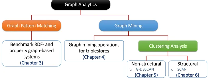
Figure 1.1 summarizes our contributions and related chapters in this thesis.

Graph Pattern Matching Graph Mining

Graph Analytics

Benchmark RDF- and property graph-based

systems (Chapter 3)

Graph mining operations for triplestores

(Chapter 4)

Clustering Analysis

Non-structural

o G-DBSCAN

(Chapter 5)

Structural

o SCAN

(Chapter 6)

(16)

1.3 Outline

(17)

Chapter 2

Modern Graph Analytics

2.1 Graph and Graph Data Models

Many real-world problems originating from computational sciences can be efficiently and in-tuitively represented as graphs. Example scientific disciplines that deal with graphs include, but not limited to, cheminformatics, bioinformatics, geoinformatics, astronomy, meteorology, material science, and geology. For example, in bioinformatics alone, graphs are applied to metabolic pathways, signaling pathways, gene regulatory networks, partonomies, chemical struc-ture graphs, gene clustering, and topological adjacency relations [69]. A formal definition of a graph is shown in Definition 1.

Definition 1 G = (V, E) is a graph where V is a set of elements and E is a relation where

E ⊆ V ×V. The elements of V are called nodes (or vertices) and the elements of E are called

edges.

If edges in a graph have directions, the graph is called a directed graph and defined as shown in Definition 2

Definition 2 A graph G = (V, E) is a directed graph if there is an arc from a node u to a

node v where (u, v)∈ E.

A labeled graph is a graph whose nodes and edges have labels and defined as shown in

Defini-tion 3.

Definition 3 A labeled graph G = (V, E, LV, LE, µ, ν) is a graph that has four additional

tuples:LV,LE,µ, andν where LV is a set of node labels,LE is a set of edge labels,µ: V→ LV

is a node labeling function, and ν: E → LE is an edge labeling function. Specifically, a graph

G = (V, E, LV, µ) is called a node-labeled graph and a graph G = (V, E,LE, ν) is called an

(18)

If entities in a labeled graph have attributes associated to them, the graph is called a property

graph and defined as shown in Definition 4.

Definition 4 A property graph G = (V, E, LV, LE, AV, AE,µ, ν) is a labeled graph that has

two additional tuples:AV and AE where AV is a set of node attributes and AE is a set of edge

attributes.

For aided graph processing, it is required that graphs are represented in computer-readable forms. Currently, matrix,Resource Description Framework (RDF) [31], and property

graph [10] are frequently used for this purpose. First, matrix is a traditional way to represent

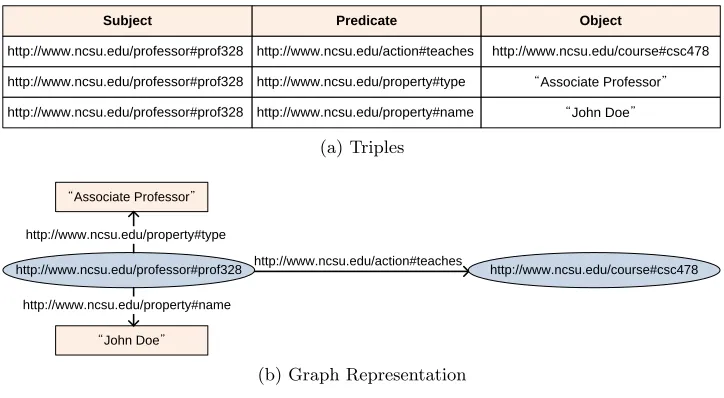
graphs, and adjacency matrix and adjacency list are two representative data structures. In this model, it is complicated to assign attributes to graph entities except edge weights without special data structures. Next, RDF was established by the World Wide Web Consortium (W3C), and is a key standard for representing and linking resource on the Web. The basic unit in this model is a triple of<subject, predicate, object>. Each triple (1) represents two resources on the Web and their relationship or (2) gives a resource an attribute. For example, assuming a university scenario, a statement “an associate professor in North Carolina State University whose name is

John Doe teaches CSC478” can be represented with a set of triples as shown in Figure 2.1(a).

Note that resources and relation types are URIs, which can uniquely identify them on the

Subject Predicate Object

http://www.ncsu.edu/professor#prof328 http://www.ncsu.edu/action#teaches http://www.ncsu.edu/course#csc478

http://www.ncsu.edu/professor#prof328 http://www.ncsu.edu/property#type “Associate Professor”

http://www.ncsu.edu/professor#prof328 http://www.ncsu.edu/property#name “John Doe”

(a) Triples

“Associate Professor”

http://www.ncsu.edu/professor#prof328 http://www.ncsu.edu/action#teaches http://www.ncsu.edu/course#csc478 http://www.ncsu.edu/property#type

“John Doe”

http://www.ncsu.edu/property#name

(b) Graph Representation

Figure 2.1. RDF Triples and Graph Representation

(19)

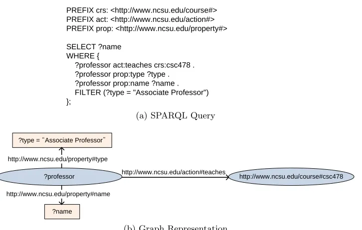
RDF graphs are managed by dedicated database management systems, calledtriplestores [45, 70, 25, 96, 60]. While those systems depend on different back-end processing platforms includ-ing RDBMS, NoSQL, clusters, and shared-memory supercomputers, they provide an logical view of triples and a standard query interface. The query interface allows users to interact with triplestores for managing and querying RDF data. The standard query language is called

SPARQL[79] and it provides a declarative way for users to describe their queries. For example,

a query to find the names of associate professors who teach CSC478 can be written in SPARQL as shown in Figure 2.2(a), which can be represented as a graph shown in Figure 2.2(b).

PREFIX crs: <http://www.ncsu.edu/course#> PREFIX act: <http://www.ncsu.edu/action#> PREFIX prop: <http://www.ncsu.edu/property#>

SELECT ?name WHERE {

?professor act:teaches crs:csc478 . ?professor prop:type ?type . ?professor prop:name ?name . FILTER (?type = "Associate Professor") };

(a) SPARQL Query

?type = “Associate Professor”

?professor http://www.ncsu.edu/action#teaches http://www.ncsu.edu/course#csc478 http://www.ncsu.edu/property#type

?name

http://www.ncsu.edu/property#name

(b) Graph Representation

Figure 2.2. An Example SPARQL Query

1

type: “associate professor” name: “John Doe”

7

teaches

2

course: “csc478” year: 2016

Figure 2.3. An Example Property Graph

(20)

sys-tems such asDex [59],Neo4j [100],TitanDB[88], andGraphX [104]. As defined in Definition 4, nodes and edges have attributes (or properties) and they are assigned to those entities as key-values pairs. Figure 2.3 shows an example of property graph. Unlike RDF, there is no standard for graph serialization and query interface in this model.

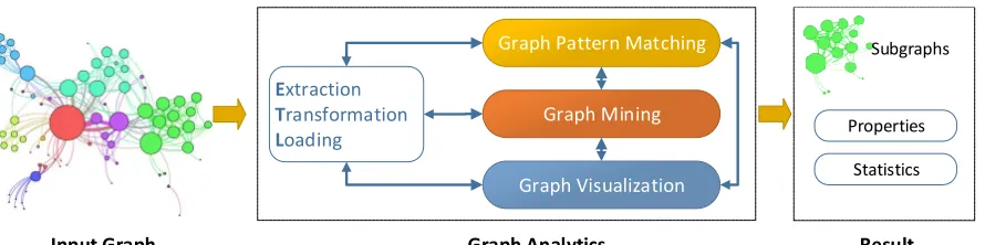
2.2 Graph Analytics

Extraction

Transformation

Loading

Graph Pattern Matching

Graph Mining

Graph Visualization

Subgraphs

Properties

Statistics

Input Graph Graph Analytics Result

Figure 2.4. Graph Analytics Process

Once real-world entities along with their ties/interactions have been modeled as graphs, routine tasks over such graph databases are analyzing them to discover valuable associations and properties, which positions graph analytics at the center of recent data analytics. For example, biologists examine protein-protein interaction graphs to investigate biological processes within a cell with various methods [75]. In social network analysis, it is an important task to identify and characterize special or exceptional relationships between social entities [7]. Figure 2.4 illustrates the general graph analytics process [51]. An interesting graph is extracted from data sources, transformed into a suitable form the target graph analysis system can process, and loaded into the system (ETL process). Then, the loaded graph is analyzed with three core tasks: graph

pattern matching,graph mining, and graph visualization [110, 51, 32, 2, 38].

Graph pattern matching aims at finding interesting subgraphs occurred in graphs. Users can describe graph patterns through query/programming interfaces systems provide, and those patterns also form graphs as shown in Figure 2.2(a). Structural graph pattern matching is defined in terms of graph isomorphism [46].

Definition 5 Graphs G and H are isomorphic if there is a bijection, f, that maps the node sets

of G and H such that two nodes u and v are adjacent in G if and only if f(u) and f(v) are also

(21)

Definition 5 shows that graph pattern matching aims to find all matched subgraphs in a graph G which are isomorphic to a given pattern P. The pattern P specifies structural constraints. In this thesis, we consider real-world graphs, which require additional constraints on node and edge labels and attributes [32].

Graph mining is another important task in graph analytics that aims to uncover hidden knowledge and obscure properties from graph databases [51, 1]. It consists of various operations which can be grouped into multiple categories according to their goals. Those categories include classification [55] and clustering [27, 105] that can be observed in traditional data mining. On the other hand, graph structures result in unique properties such as diameter, degree, and eccentricity to be mined [94, 8, 46], and bring about additional operation categories such as link analysis [72, 56]

Representing graphs in visualized forms is a key task for graph discovery process [38]. This task gives an intuitive way for data scientists to explore graph structures in an interactive manner. For example, they can iteratively figure out interesting parts of a graph and move to those parts for further exploration with visualization tools or export them for continuous anal-ysis. Recent large scale graphs especially demand fast algorithms and effective representation formats [42, 81]. Note that we focus only on graph pattern matching and graph mining in this thesis.

In real-world graph analytics, graph pattern matching, graph mining, and graph visualiza-tion are cooperatively and interchangeably performed on graph databases. For example, graph pattern matching can be used forgraph filtering [107] anddimensionality reduction [2] in order to reduce the computational complexity of following graph mining operations. In another exam-ple, new properties such as ranks and centrality scores computed by graph mining operations can augment graphs and used for filtering graph entities for graph pattern matching. Those tasks are repeated until data scientists perform enough exploration and, hence, gather desired results.

2.3 Modern Graph Processing Systems

(22)

high-performance clusters, and uRiKA-GD [60] is a shared memory graph processing supercomputer. Those systems rely on different graph data models such as matrix [101, 93, 15], RDF [45, 70, 96, 60], and property graph [34, 23, 88, 83]. Those systems are also backed on various storage sub-systems including in-memory [34], relational database systems, and NoSQL, and provide different query/programming interfaces such as general programming languages, SPARQL [79], Cypher [40], Gremlin [39], and so on.

(23)

Chapter 3

Benchmark Graph Analysis Systems

with Graph Pattern Matching

Workloads

As discussed in Chapter 2, the advent of recent graph analysis systems broadens options that data scientists can select for their graph analytics tasks. Those systems show diversities in terms of graph data models, system architectures, query interfaces, and graph serialization formats. The presence of such diversity makes users to perform ad-hoc evaluations with desired workloads. Specifically, such evaluations require multiple fastidious steps: transforming datasets into several different serialization formats, loading datasets into systems via different interfaces, and writing and customizing queries in different query languages. Hence, a full investigation into each system is problematic in that it is time consuming, error-prone, and can easily cause a deviation from the ultimate goal.

This study aims at providing an evaluation of recent six graph analysis systems with graph pattern matching workloads. More specifically, we focus on graph analysis systems which are based on the two popular graph models: RDF and property graph. In order to provide full understandings of those systems, we compare those systems in terms of not only graph pattern matching performance but also different aspects of importance such as expressiveness of query languages, optimization, graph serialization, and before-and-after graph data size.

3.1 Benchmarked Graph Analysis Systems

(24)

a triplestore, which is built around a shared-memory supercomputer architecture, previously known as the Cray XMT. The software stack of the system processes each SPARQL query in parallel by leveraging a huge number of hardware threads. For example, uRiKA-512 has 512 Threadstorm IV graph accelerators (processors) with 128 hardware threads per processor [43]. It has separate 68 x86-based processors dedicated to parallel I/O. Processors are interconnected in a Cray-designed 3D torus network.

Property graph-based systems are broadly categorized into two classes. First, graph database systems are designed specifically for optimal graph data store and retrieval over NoSQL database systems. Examples in this class include Dex [59], Neo4j [23], and Titan [88]. Second, systems such as NetworkX [34], and GraphX [104] are general purpose graph processing systems and typically focus on graph analysis rather than transactional graph data management. Each of those systems provides a distinct computation model and built-in graph mining operations opti-mized to the model. For property graph-based systems, there is no standardized query interface. For example, Neo4j and Titan provide their own query languages called Cypher [40] and Grem-lin [39], respectively. NetworkX, itself, is a Python library for in-memory graph analysis and the general programming interface of Python is the only way to write graph analysis queries. GraphX is another graph analysis library running on top of Spark [109]. GraphX queries are written in several programming languages such as Python and Scala by using built-in data structures and operations.

3.2 Benchmark Suite Design

For comprehensive evaluations, it is inevitable to rely on a benchmark suite that supports various graph serialization formats and query languages while managing the structural charac-teristics of benchmark datasets as the same. However, existing graph benchmark suites do not satisfy those requirements. Therefore, we developed a benchmark suite by extending a popular benchmark suite for triplestores calledLehigh University Benchmark (LUBM) [33]. The exten-sion supports several graph serialization formats and benchmark queries in different languages for property graph-based systems. In this section, we explain the benchmark suite and introduce our extension.

3.2.1 LUBM Benchmark Suite

(25)

< ub : D e p t rdf : a b o u t = " h t t p :// www . D e p t 0 . U n i v 0 . edu " > < ub : name > Dept0 </ ub : name >

< ub : s u b O r g a n i z a t i o n O f >

< ub : U n i v rdf : a b o u t = " h t t p :// www . U n i v 0 . edu " / > </ ub : s u b O r g a n i z a t i o n O f >

</ ub : Dept >

Listing 3.1. Example Data in OWL

by using sameseed parameter values. They simulate a university use-case where entities in uni-versities are represented as nodes and their associations as edges. The unit of data generation is a university and the number of universities is used as a scale factor. In each university, entities such as students, professors, and departments are randomly connected within certain ranges of degree. The details on the data profile of LUBM can be found at [36]. The benchmark query set consists of 14 queries written in SPARQL, each of which shows different selectivity, complexity, class hierarchy, and inference requirement.

3.2.2 Extension for Data Generation

LUBM datasets are generated in two serialization formats in RDF and they are rarely sup-ported by current property graph-based systems. In addition, triplestores often require differ-ent formats for data loading. Hence, we extend the LUBM data generator so that it is able to generate benchmark datasets in several graph serialization formats. For triplestores, the ex-tension generates datasets in N-triple, which is an RDF data exchange format supported by the majority of current triplestores. For property graphs, however, it is not straightforward to generate datasets, preserving the relevance of semantics with minimizing redundancy while supporting current graph analysis systems. This is because (1) there is no standard for graph serialization formats, and (2) different systems have their own requirements on serialized graph structure even though they have a common serialization format. Specifically, GraphML [30] is supported by NetworkX and Neo4j but not by GraphX. In addition, Neo4j strictly expects node descriptions to be placed before edges descriptions in a GraphML document. Addressing such difficulties, our extended data generator produces property graphs in two serialization formats which are GraphML formatted to be compatible with NetworkX and Neo4j and

Prop-erty Graph/JSON [50] for GraphX. For example, Listing 3.1 shows an example data in OWL

(26)

< key id = " n a m e " for = " n o d e " a t t r . n a m e = " n a m e " a t t r . t y p e = " s t r i n g " / > < key id = " t y p e " for = " n o d e " a t t r . n a m e = " t y p e " a t t r . t y p e = " s t r i n g " / > < key id = " uri " for = " n o d e " a t t r . n a m e = " uri " a t t r . t y p e = " s t r i n g " / >

< key id = " s u b O r g a n i z a t i o n O f " for = " e d g e " a t t r . n a m e = " s u b O r g a n i z a t i o n O f " a t t r . t y p e = " s t r i n g " / > ...

< n o d e id = " h t t p :// www . D e p t 0 . U n i v 0 . edu " l a b e l s = " D e p t " > < d a t a key = " uri " > h t t p :// www . D e p t 0 . U n i v 0 . edu </ data > < d a t a key = " t y p e " > Dept </ data >

< d a t a key = " n a m e " > Dept0 </ data > </ node >

...

< e d g e id = " s u b O r g a n i z a t i o n O f " l a b e l = " s u b O r g a n i z a t i o n O f "

s o u r c e = " h t t p :// www . D e p t 0 . U n i v 0 . edu " t a r g e t = " h t t p :// www . U n i v 0 . edu " > </ edge >

Listing 3.2. Example Data in GraphML

// n o d e s . j s o n {

" id " : " h t t p :// www . D e p t 0 . U n i v 0 . edu " , " t y p e " : " D e p t " ,

" n a m e " : " D e p t 0 " }

// e d g e s . j s o n {

" s o u r c e " : " h t t p :// www . D e p t 0 . U n i v 0 . edu " , " t a r g e t " : " h t t p :// www . U n i v 0 . edu " , " t y p e " : " s u b O r g a n i z a t i o n O f " }

Listing 3.3. Example Data in Property Graph/JSON

in property graph-based systems. Therefore, we add an additional “uri” attribute in GraphML so that nodes can be identified with their URIs in queries. We add a “labels” attribute to each “node” element for Neo4j to recognize the type of the node. Each edge has its ID, and source and destination nodes’ URIs which are encoded as internal numeric IDs. We add an “label” attribute to represent the types of edges since it is required to retrieve edges by their types.

The extended data generator also produces datasets in Property Graph/JSON for GraphX. Nodes and edges are serialized in two separate files: nodes.json and edges.json as shown in Listing 3.3. Since GraphX does not provide a Property Graph/JSON data loader, we imple-mented a custom loader. It loads the two files and generates a graphRDD (Resilient Distributed

Dataset), which is the data structure for GraphX. Each graph entity is declared between{ and

}and each attribute is represented as attribute name: attribute value. Attributes are delimited by commas. Since URIs are replaced with unique internal IDs when data are loaded, they are stored as separate attributes.

(27)

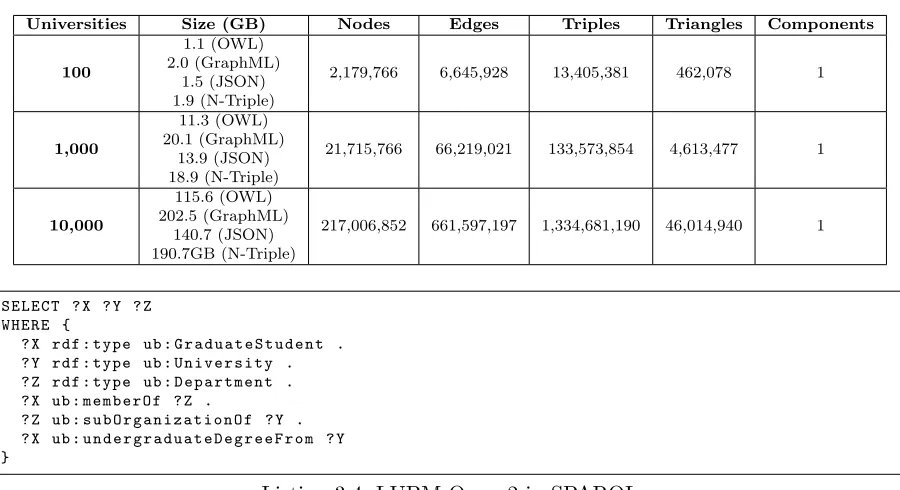
Table 3.1. Characteristics of Datasets

Universities Size (GB) Nodes Edges Triples Triangles Components

100

1.1 (OWL) 2.0 (GraphML)

1.5 (JSON) 1.9 (N-Triple)

2,179,766 6,645,928 13,405,381 462,078 1

1,000

11.3 (OWL) 20.1 (GraphML)

13.9 (JSON) 18.9 (N-Triple)

21,715,766 66,219,021 133,573,854 4,613,477 1

10,000

115.6 (OWL) 202.5 (GraphML)

140.7 (JSON) 190.7GB (N-Triple)

217,006,852 661,597,197 1,334,681,190 46,014,940 1

S E L E C T ? X ? Y ? Z W H E R E {

? X rdf : t y p e ub : G r a d u a t e S t u d e n t . ? Y rdf : t y p e ub : U n i v e r s i t y . ? Z rdf : t y p e ub : D e p a r t m e n t . ? X ub : m e m b e r O f ? Z .

? Z ub : s u b O r g a n i z a t i o n O f ? Y . ? X ub : u n d e r g r a d u a t e D e g r e e F r o m ? Y }

Listing 3.4. LUBM Query2 in SPARQL

number of triangles are proportional to the number of universities while the generated graphs have a single connected component. In each dataset, triples corresponding to node properties occupy 50% of the total number of triples. Different formats result in different sizes of generated datasets. For example, GraphML produces the largest datasets to represent the same graphs.

3.2.3 Query Translation

While triplestores have a standard query interface, property graph-based systems provide differ-ent query interfaces. Hence, it is necessary to rewrite the benchmark queries in several languages to compare those systems. For query selection and rewriting, we took the approach proposed in [32]. We selected 9 queries out of 14 original LUBM queries and those queries were written in two query languages (Cypher and Gremlin) and two general programming languages (Python with NetworkX and Scala with GraphX).

Cypher is the default query language of Neo4j. It is designed to describe graph patterns and provides an intuitive way similar to SPARQL, which allowed us to rewrite queries with a minimal effort. Listing 3.5 shows the LUBM query2 in Cypher which is translated from the original SPARQL query in Listing 3.4.

(28)

M A T C H

( x : G r a d u a t e S t u d e n t ) -[: m e m b e r O f ] - >( z : D e p a r t m e n t ) , ( z ) -[: s u b O r g a n i z a t i o n O f ] - >( y : U n i v e r s i t y ) ,

( x ) -[: u n d e r g r a d u a t e D e g r e e F r o m ] - >( y ) R E T U R N

x . uri , y . uri , z . uri ;

Listing 3.5. LUBM Query2 in Cypher

g r a p h . V . f i l t e r { it . t y p e == ’ G r a d u a t e S t u d e n t ’ } . as ( ’ g r a d u a t e _ s t u d e n t ’ )

. out ( ’ m e m b e r O f ’ ). f i l t e r { it . t y p e == ’ D e p a r t m e n t ’ } . out ( ’ s u b O r g a n i z a t i o n O f ’ )

. f i l t e r { it . t y p e == ’ U n i v e r s i t y ’ } . inE ( ’ u n d e r g r a d u a t e D e g r e e F r o m ’ ) . o u t V . r e t a i n ( ’ g r a d u a t e _ s t u d e n t ’ )

. s i d e E f f e c t { f < < "${ it . uri }\ r \ n " }. i t e r a t e ()

Listing 3.6. LUBM Query2 in Gremlin

as a collection of predefined steps each of which maps to a particular pipe operation as shown in Listing 3.6. Chaining pipes creates a pipeline where graph entities are processed through the pipeline. Each pipe operation broadly falls into four categories:transform,filter,sideEffect, andbranch. Steps can easily represent a traverse along edges in a graph. It also provides a few primitives that allow such traversals to resume from previous steps such asbackand reference intermediate records produced at previous steps such asretain. Gremlin especially focuses on graph traversals and this makes it less straightforward to write graph pattern matching queries. We discuss the limitations of the language for writing pattern matching queries in Section 3.3.3. Listing 3.7 shows the query2 implementation in Python with NetworkX. Describing graph patterns in NetworkX requires iterating nodes in graphs and, in turn, edges for each node. This often resulted in nested loops for writing the benchmark queries via the given interface.

for x in g r a p h :

if x [ ’ t y p e ’ ] == ’ G r a d S t u d e n t ’ : for e d g e in g r a p h . e d g e s ( x ):

if e d g e [ ’ t y p e ’ ] = ’ u n d e r g r a d u a t e D e g r e e F r o m ’ : y = e d g e . n e i g h b o r

if e d g e [ ’ t y p e ’ ] = ’ m e m b e r O f ’ : z = e d g e . n e i g h b o r

if y and z are m a t c h e d :

if y [ ’ t y p e ’ ] == ’ U n i v e r s i t y ’ : if z [ ’ t y p e ’ ] == ’ D e p a r t m e n t ’ :

if g r a p h . h a s _ e d g e ( y , z , ’ s u b O r g a n i z a t i o n O f ’ ): p r i n t x , y , z

(29)

val m e m b e r O f = g r a p h . t r i p l e t s . f i l t e r ( t r i p l e t = > (

t r i p l e t . s r c A t t r . t y p e == " G r a d u a t e S t u d e n t " && t r i p l e t . d s t A t t r . t y p e == " D e p a r t m e n t " && t r i p l e t . a t t r == " m e m b e r O f "

) ). map {

t r i p l e t = > ( t r i p l e t . srcId , ( t r i p l e t . s r c A t t r . uri , t r i p l e t . dstId , t r i p l e t . d s t A t t r . uri )) }

val u n d e r g r a d u a t e D e g r e e F r o m = g r a p h . t r i p l e t s . f i l t e r ( t r i p l e t = > (

t r i p l e t . s r c A t t r . t y p e == " G r a d u a t e S t u d e n t " && t r i p l e t . d s t A t t r . t y p e == " U n i v e r s i t y " &&

t r i p l e t . a t t r == " u n d e r g r a d u a t e D e g r e e F r o m " )

) ...

val s u b O r g a n i z a t i o n O f = ...

# j o i n i n g t r i p l e t s to r e t r i e v e p a t t e r n s

val t e m p = m e m b e r O f . j o i n ( u n d e r g r a d u a t e D e g r e e F r o m ) ...

val r e s u l t = t e m p . j o i n ( s u b O r g a n i z a t i o n O f ) ...

Listing 3.8. LUBM Query2 in Scala with GraphX

GraphX provides a set of graph processing primitives that can be used for graph analysis. For describing LUBM queries, we extensively usedtripletandjoin. Triplet, which is inspired by RDF triples, provides a node-edge-node view of a graph and an object-oriented view of triplet for accessing attributes of graph entities.filterand mapoperations are used to select triplets that we are interested in and transform them into desired structure. Then the connection of the selected triplets is performed by join operations. Listing 3.8 shows the simplified code of LUBM query2 for GraphX.

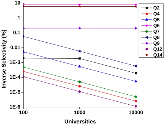
The benchmark queries have different properties in terms of structure and selectivity. For example, those queries have different pattern structures as shown in Table 3.2. “Neighborhood” is a basic triple pattern which consists of a node and its neighbor. ”Chain” is a pattern consisting of multiple triples where the object of a pattern is the subject of another pattern. “Star” consists of a subject and multiple objects connected to it and “Triangle” consists of three triples where three nodes are adjacent to each other forming a triangle. Figure 3.1 shows the inverse selectivity of the queries in log scale, which is computed as

inverse selectivity= number of output records

(30)

Table 3.2. Structural Properties of Benchmark Queries.

Pattern Q2 Q4 Q5 Q6 Q7 Q8 Q9 Q12 Q14

Neighborhood O O O X O O O O X

Chain O X X X X O O O X

Star O O X X X O O X X

Triangle O X X X X X O X X

Multi-edge X X O X X X X O X

Inference X O O O O O O O X

same rate as input size increases. Q2 produces more output records when universities = 1,000 than universities = 100 but the same number of output records when universities = 10,000.

1 0 0 1 0 0 0 1 0 0 0 0

1 E - 6 1 E - 5 1 E - 4 1 E - 3 0 . 0 1 0 . 1

1

1 0

In

v

e

rs

e

S

e

le

c

ti

v

it

y

(

%

)

U n i v e r s i t i e s

Q 2 Q 4 Q 5 Q 6 Q 7 Q 8 Q 9 Q 1 2 Q 1 4

Figure 3.1. Inverse Selectivity of Queries in Log Scale

3.3 Benchmark Results

(31)

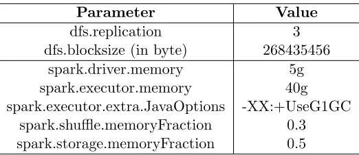
Table 3.3. Parameters for HDFS and Spark

Parameter Value

dfs.replication dfs.blocksize (in byte)

3 268435456 spark.driver.memory

spark.executor.memory spark.executor.extra.JavaOptions

spark.shuffle.memoryFraction spark.storage.memoryFraction

5g 40g -XX:+UseG1GC

0.3 0.5

3.3.1 Evaluation Environments

In this benchmark, we selected NetworkX 1.9.1, Jena Fuseki 1.1.1 with TDB (a disk-based native store), Neo4j 2.2.3 community edition as standalone graph analysis systems. Those systems were tested on a desktop that has an i5 1.3GHz quad-core processor, 16GB DDR3 RAM, and a 250GB solid state disk. For Java-based systems (Jena and Neo4j), we configured the JVM maximum heap size to 80% of the physical memory.

For high-performance systems, we tested GraphX packaged in Spark 1.3.1, Titan 0.5.1 with HBase 1.0 as the backend storage, and uRiKA-64. GraphX and Titan were tested on a cluster at Oak Ridge National Laboratory consisting of 9 virtual machines from CADES (Compute

and Data Environment for Science) [49]. Each virtual machine has 32 virtual processors, 64GB

RAM, and a 500GB local disk. For the underlying storage, we used Hadoop Distributed File System (HDFS) which is packaged in Hadoop 2.4.0. For both systems, we used 8 worker nodes (region servers for HBase). For Titan, we used three nodes of zookeeper quorum with all default parameters. We configured HDFS and Spark as shown in Table 3.3. We used a uRiKA-64 system at Oak Ridge National Laboratory. It is a supercomputer-based graph analysis system and has a 2TB shared-memory, 8,192 hardware threads, and 125TB Lustre file system.

3.3.2 Quantitative Evaluation

(32)

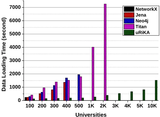
data loading after 12 hours. As many property graph-based systems, Titan internally allocates IDs for node and edge entities. It allocates a block of IDs ahead of creating entities. However, those pre-allocated IDs are depleted too soon compared to the data ingestion rate of back-end storages. In addition, the use of HBase backend contributed to linear increase of loading time. When inserting a new entry, it first fills a region in one region server. When the region size exceeds a configured limit, the region splits. Then, if the number of regions in the region server exceeds a limit, it finds a new region in another region server. Therefore, the loading process did not fully utilize multiple region servers when we bulk-load graphs. In uRiKA, multiple I/O processors enabled concurrent data loading and database creation. This parallelized I/O and data processing capability resulted in the best data loading performance out of the five systems.

1 0 0 2 0 0 3 0 0 4 0 0 5 0 0 1 K 2 K 3 K 4 K 5 K 1 0 K

0

1 0 0 0 2 0 0 0 3 0 0 0 4 0 0 0 5 0 0 0 6 0 0 0 7 0 0 0

D

a

ta

L

o

a

d

in

g

T

im

e

(

s

e

c

o

n

d

)

N e t w o r k X J e n a N e o 4 j T i t a n u R i K A

Figure 3.2. Data Loading Time

(33)

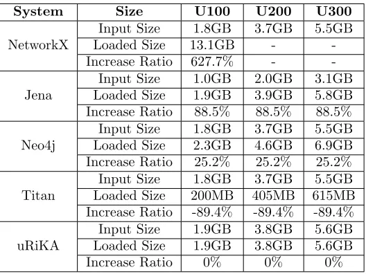
Table 3.4. Before-and-after Graph Size Changes

System Size U100 U200 U300

Input Size 1.8GB 3.7GB 5.5GB

Loaded Size 13.1GB -

-NetworkX

Increase Ratio 627.7% -

-Input Size 1.0GB 2.0GB 3.1GB

Loaded Size 1.9GB 3.9GB 5.8GB

Jena

Increase Ratio 88.5% 88.5% 88.5%

Neo4j

Increase Ratio 25.2% 25.2% 25.2%

Loaded Size 200MB 405MB 615MB

Titan

Increase Ratio -89.4% -89.4% -89.4%

uRiKA

Increase Ratio 0% 0% 0%

uRiKA, it stores graphs as in their input formats, which resulted in no change on the graph size.

(34)

(35)