INVESTIGATION
Multiple Adaptive Substitutions During Evolution
in Novel Environments
Kavita Jain*,†,1and Sarada Seetharaman* *Theoretical Sciences Unit and†Evolutionary and Organismal Biology Unit, Jawaharlal Nehru Centre for Advanced Scientific Research, Bangalore 560064, India
ABSTRACTWe consider an asexual population under strong selection–weak mutation conditions evolving on ruggedfitness
land-scapes with many localfitness peaks. Unlike the previous studies in which the initialfitness of the population is assumed to be high, here we start the adaptation process with a lowfitness corresponding to a population in a stressful novel environment. For generic fitness distributions, using an analytic argument wefind that the average number of steps to a local optimum varies logarithmically with the genotype sequence length and increases as the correlations among genotypic fitnesses increase. When thefitnesses are exponentially or uniformly distributed, using an evolution equation for the distribution of populationfitness, we analytically calculate thefitness distribution offixed beneficial mutations and the walk length distribution.
A
DAPTATION is an evolutionary process during which a population improves itsfitness by accumulating bene-ficial mutations. A population of genotypic sequences produ-ces a suite of mutants and if better mutants become available, a maladapted population may acquire one of the beneficial mutations provided it does not get lost due to genetic drift. The fitter population in turn may acquire another advanta-geous mutation and the process goes on until the supply of beneficial mutations gets exhausted. A number of models with variable degrees of biological consistency have been proposed and investigated to understand the process of adaptation (Milleret al.2011). One of the simplest mathematical models was introduced by Gillespie in which beneficial mutations arise sequentially and fix rapidly (Gillespie 1991). If the mutation rate is small and the selection coefficient is large (compared to the inverse population size), it is a good ap-proximation to assume that only the one-step mutants are accessible at any time and the population is localized at a sin-gle genotype. Such a monomorphic population performs an adaptive walk by moving uphill on afitness landscape until no more beneficial mutations can be found.In the last few years, much of the work on Gillespie’s model has focused on the first step in the adaptation pro-cess. If the fitnesses of the wild type and its one-mutant neighbors are rank ordered with the fittest sequence at the top, the well established theory of extremes of independent random variables (David and Nagaraja 2003) can be exploited to obtain useful information provided the wild type has a highfitness (rank). For a moderately high-ranked initial fitness, Orr calculated the expected rank at the first step as-suming exponential-likefitness distributions (Orr 2002). His prediction has been tested in an experiment using single-stranded DNA and found to be roughly consistent with the experimental data (Rokytaet al.2005). This result has been later generalized for other fitness distributions (Joyceet al. 2008) and by including correlations among fitnesses (Orr 2006). However, as the properties of the entire walk are re-quired to design a drug or a biomolecule (Bull and Otto 2005) and as experimental data on multiple adaptive substi-tutions are becoming available (Rokytaet al.2009; Schoustra et al. 2009), it is important to extend the existing theory to address the statistical properties of the entire walk.
With this aim, we study Gillespie’smutational landscape modelon ruggedfitness landscapes with many localfitness optima. An important difference between our work and the previous ones is that here we start the adaptive walk with lowfitness to describe the adaptation process in novel envi-ronments such as when antibiotics are introduced (MacLean and Buckling 2009; McDonald et al. 2010) whereas the
Copyright © 2011 by the Genetics Society of America doi: 10.1534/genetics.111.134163
Manuscript received July 19, 2011; accepted for publication August 29, 2011
1Corresponding author: Theoretical Sciences Unit and Evolutionary and Organismal
initial fitness is assumed to be high in other studies (Gillespie 1991; Orr 2002,2006; Joyceet al.2008). Several
numerical (Gillespie 1991; Orr 2006) and experimental studies (Rokytaet al.2009; Schoustraet al.2009) have in-dicated that only a few steps are required to reach a local optimum. In a simple adaptation model that assumes the mutational neighborhood remains unchanged during the entire adaptive walk (Gillespie 1983), the average number of steps to a localfitness peak has been calculated analyti-cally for variousfitness distributions and shown to increase logarithmically with the rank of the initial sequence (Neidhart and Krug 2011). However, here we work with a more realistic mutation scheme in which a new suite of mutants is created in each adaptive step. For genericfitness distributions, we argue that the average number of adaptive steps increases logarithmically with sequence length with a prefactor that depends on the choice offitness distribution. Although our argument does not capture the proportionality constant correctly, the logarithmic dependence is seen to be in excellent agreement with the simulation results. We also present detailed results on the statistical properties of the entire walk for exponentially and uniformly distributed fitnesses as these two distributions lend themselves to an analytic treatment and are also consistent with the experi-ments (Eyre-Walker and Keightley 2007; Rokyta et al. 2008). Following the approach of Flyvbjerg and Lautrup (1992), we write a recursion relation for the fitness distri-bution offixedbeneficial mutations at an adaptive step that is valid for long sequences and fitness distributions with a finite mean. A similar distribution has been calculated in the clonal interference regime in which multiple mutants are produced per generation (Rozen et al. 2002) while here we work in the weak mutation regime. For the above-mentioned distributions, we also find the distribution of walk length. The average walk length calculated using this approach gives a prefactor consistent with the numerical results.
Although for most of the article we work with uncor-related fitnesses and assume that the distribution of the fitness does not change during the course of evolution, the effect of correlations is also discussed. As experiments support an intermediate degree of correlations in fitness landscapes (Carneiro and Hartl 2010; Miller et al. 2011) and changingfitness distributions may be modeled by cor-related fitnesses (Orr 2006), we calculate the average number of steps to an optimum on afitness landscape gen-erated by the block model of correlatedfitnesses in which a sequence is divided into several independent blocks and correlations arise when two sequences share some blocks (Perelson and Macken 1995). The average walk length has been measured using numerical simulations in a block model in Orr (2006) and it was speculated that the average number of adaptive steps is independent of the underlying fitness distribution and increases linearly with the number of blocks. We show that while the latter result is roughly correct, the average number of steps to a local optimum is
not independent of thefitness distribution, which is a con-sequence of the result discussed above for the uncorrelated fitness landscapes.
Models and Methods
Uncorrelated and correlatedfitness landscapes
An uncorrelated fitness landscape can be generated by assigning a fitness to a sequence independent of that of other sequences. Thefitnesses are sampled from a common distributionp(f) with support on the interval [l,u]. Although the full distribution of absolutefitness is unknown, one can obtain an insight into its nature through the distribution of beneficial mutations that has been measured in several the-oretical and experimental studies (Eyre-Walker and Keightley 2007). A theoretical argument suggests that since good mutations are rare, their distribution is governed by the upper tail of the fitness distribution p(f) (Gillespie 1991). It is known from the extreme value theory (EVT) for inde-pendent and identically distributed (i.i.d.) random variables that the asymptotic distribution of the extreme value can be one of the following three types (David and Nagaraja 2003): Frechet for algebraically decaying underlying distributions, Gumbel for unbounded distributions decaying faster than a power law, and Weibull for bounded distributions. To be consistent with this result, we make the following choices for thefitness distributions:
pðfÞ ¼
8 < :
ðd21Þð1þfÞ2d; d.2 ðFrechetÞ ð1Þ gfg21e2fg; g.0 ðGumbelÞ ð2Þ nð12fÞn21; n.0;f,1 ðWeibullÞ ð3Þ:
The conditiond.2 in (1) is imposed to keep the transition rate (6)finite (as explained later). The last twofitness func-tions (2) and (3) are of particular interest as several exper-imental results on the distribution of beneficial mutations have been found to lie in the Gumbel domain (Imhof and Schlotterer 2001; Sanjuán et al. 2004; Rokyta et al. 2005;
Kassen and Bataillon 2006; MacLean and Buckling 2009) and a recent work finds a best fit for the distribution of beneficial effects to a uniform distribution that lies in the Weibull domain (Rokytaet al.2008).
corresponding i.i.d. class even if correlations are weak (Jain et al.2009; Jain 2011). In the following discussion, we as-sume that the sequence fitnesses are uncorrelated and deal with the correlated fitnesses in the last subsection of next section.
Adaptive walk model for long sequences
We work with haploid binary sequences of length Lin the strong selection–weak mutation (SSWM) regime. IfNis the population size, the SSWM regime corresponds to Ns?1, Nm>1 where s is the selection coefficient and m is the mutation probability per locus per generation. Since the expected number of mutants produced per generation is much smaller than one, mutations occur sequentially and double and higher mutations may be neglected. Thus the mutational neighborhood of a sequence is limited to L mutants that are a single mutation away from it. If the fi t-nesses of the wild-type sequence and itsLone-mutant neigh-bors are arranged in a descending order with the bestfitness assigned the rank 1, the transition probability that the pop-ulation moves from the wild type with fitness rank i and valuefito a mutant with rankj,iand valuefjis propor-tional to thefixation probability, which is well approximated by 2(fj2fi)/fiin the strong selection limit (Gillespie 1991). The normalized transition probability from fitness fi to fi t-nessfjis given by
T
fj)fi
¼ fj2fi Pi21
k¼1fk2fi
; 1#j#i21: (4)
Once the population has moved to a mutant sequence with fitnessfjwith probabilityT(fj)fi), it produces a set of new mutants that are rank ordered and chosen according to (4) and the process repeats itself until the population reaches a local optimum whose nearest neighbors are all lessfit than itself. Note that the parametersNandmhave dropped out of the picture and the properties of the model depend on the sequence length (or the initial rank) and the distribution of sequencefitnesses.
The model described above has been studied using (4) and EVT in previous works (Gillespie 1991; Orr 2002,
2006;Joyceet al. 2008) assuming the initialfitness to be
high (smalli). In contrast, we start with a lowfitness and write a recursion relation for the probabilityPJ(f) that an adaptive walk has at least J steps and the fitness is f at theJth step, following Flyvbjerg and Lautrup (1992) who studied this distribution for random adaptive walks (see Appendix A). In the following discussion, it is assumed that the sequence length is large, which allows the following two simplifications: First, the events in which a sequence is backtracked can be ignored and second, the transition rates can be written in terms of absolutefitnesses instead of fitness ranks. Consider a population at the Jth adap-tive step and with fitness h. It can proceed to the next step provided at least one fitter mutant is available. If qðhÞ ¼Rh
ldg pðgÞ, this event occurs with a probability 12
qL(h), where it is assumed that at each step in the evolu-tionary process,Lnovel mutants are available that have not been encountered before. While this is true at thefirst step, the number of novel mutants is L 21 at the second step since one of the mutants is the parent sequence itself that is not an allowed descendant as the walk always proceeds uphill. In fact for any J $ 2, some of the mutants have already been probed but the error introduced by ignoring this complication is of the order of 1/L, which is negligible for large L (Flyvbjerg and Lautrup 1992). Then for long sequences we can write
PJþ1ðfÞ ¼ Z f
l
dh pðfÞTðf)hÞ12qLðhÞPJðhÞ; J$0;
(5)
wherep(f)T(f)h) gives the probability that a mutant with fitnessf.his chosen. Furthermore for largeL, it is a good approximation to replace the sum in the denominator of (4) by an integral and we may write
Tðf)hÞ ¼Ru f2h hdgðg2hÞpðgÞ
; f.h: (6)
Thus we work with absolute fitnesses instead of fitness ranks. Since the transition probability (6) vanishes for slowly decaying fitness distributionsp(f) f2d,d # 2, we
restrictd.2 in (1). Using (6) in (5), wefinally obtain
PJþ1ðfÞ ¼ Z f
l
dhRuðf2hÞpðfÞ hdgðg2hÞpðgÞ
12qLðhÞPJðhÞ; J$0:
(7)
Equation 7 is the central equation of this article and we employ it to obtain various results on the statistical properties of adaptive walks. In the following, we assume the initial conditionP0(f) =d(f) corresponding to zero initial fitness. AsPJ(f) obeys an integral equation that is harder to analyze, we may try to write a differential equation forPJ(f). Differentiating (7) with respect tof, we get
PJ9þ1ðfÞ ¼ Z f
l
dhðfR2u hÞp9ðfÞ þpðfÞ hdgðg2hÞpðgÞ
12qLðhÞPJðhÞ;J$0
(8)
PJ99þ1ðfÞ ¼ Z f
l
dhðf2RuhÞp$ðfÞ þ2p9ðfÞ hdgðg2hÞpðgÞ
12qLðhÞPJðhÞ
þ pðfÞ
12qLðfÞ Ru
f dgðg2fÞpðgÞ
PJðfÞ; J$1; (9)
PJ99þ1ðfÞ ¼2
p9ðfÞ
pðfÞPJ9þ1ðfÞ þ
"
p99ðfÞ pðfÞ 22
p9ðfÞ pðfÞ
2#
PJþ1ðfÞ
þ pðfÞ
12qLðfÞ Ru
fdgðg2fÞpðgÞ
PJðfÞ; J$1:
(10)
The first derivative term in the above equation can be eliminated by writingPJðfÞ ¼pðfÞP~JðfÞ, whichfinally yields
~
PJ99þ1ðfÞ ¼pðfÞ
12qLðfÞ Ru
fdgðg2fÞpðgÞ
~
PJðfÞ; J$1: (11)
In this article, we restrict our attention to exponentially and uniformly distributed fitnesses as these two fitness distributions are consistent with the available empirical data. We show that due to (9), a second-order ordinary differential equation is obeyed by a generating function of PJ(f) for these two distributions, which can be solved within an approximation subject to the boundary conditions
PJðfÞjf¼l¼0; J$1 (12)
PJ9ðfÞjf¼l¼
pðlÞ
Ru
ldg g pðgÞ
dJ;1; (13)
where (12) is a direct consequence of (7) and (13) arises on using the initial condition in (8).
Besides PJ(f), we alsofind the walk length distribution
QJand the averagefitnessf
J at the Jth step, which can be related to PJ(f) as explained below. Integrating over f on both sides of (7), we get
PJþ1¼ Z u
l
df PJþ1ðfÞ (14)
¼
Z u
l
dh
Z u
h
dfRuðf2hÞpðfÞ hdgðg2hÞpðgÞ
12qLðhÞPJðhÞ (15)
¼
Z u
l
dh12qLðhÞPJðhÞ ¼PJ2 Z u
l
dh qLðhÞPJðhÞ: (16)
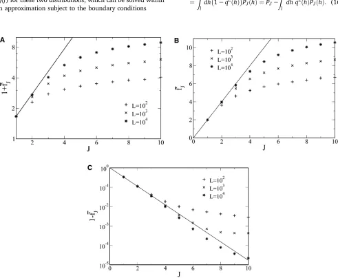
Figure 1 Evolution of averagefitness with the number of adaptive steps starting from zero initialfitness obtained numerically (points) and compared with the averagefitness in infinite sequence length limit (lines) for (A) power law-distributedfitness withd¼6, Equation 22; (B) exponentially distributed
Then the walk length probabilityQJthat exactlyJsteps are taken is given by
QJ¼PJ2PJþ1¼ Z u
l
dh qLðhÞPJðhÞ (17)
withQ0= 0 since the initialfitness is zero. The above equa-tion has a simple interpretaequa-tion: SincePJ(h) is the probability that at leastJsteps are taken and thefitness at theJth step is h, exactly J steps will be taken if all the L mutants of the sequence at the Jth step carry a fitness smaller than h from which (17) follows. The average walk length
J¼P2JL¼0JQJ PN
J¼0JQJ for largeL. The averagefitnessfJ is defined asfJ¼
Ru
ldf fPJðfÞ. Using (7), we can write
fJþ1¼
Z u
l
df f
Z f
l
dhRuðf2hÞpðfÞ
hdgðg2hÞpðgÞ
12qLðhÞPJðhÞ
(18)
¼
Z u
l
dh
12qLðhÞP JðhÞ Ru
hdgðg2hÞpðgÞ Z u
h
df fðf2hÞpðfÞ: (19)
Note that neither (17) nor (19) is a closed equation. Our analytical results are also compared with numerical simulations that were performed using an exact procedure for L#10 and an approximate method outlined in Orr (2002) for largerL. We refer the reader toAppendix Bfor details.
Results
Averagefitness and walk length for general fitness distributions
For a broad class offitness distributions, the averagefitness for an infinitely long sequence can be computed. Although this limit is biologically unrealistic, it provides a good approximation to the averagefitnessfJ for smallJ(see Fig-ure 1) as the population cannot sense thefiniteness of se-quence length far from the local optimum. On taking the limit L / N in (19) and denoting the average fitness in this limit byFJ, we obtain
FJþ1¼ Z u
l
dh
Ru
hdf fðf2hÞpðfÞ Ru
hdgðg2hÞpðgÞ
PJðhÞjL/N: (20)
Algebraically decaying fitness distributions:On
substitut-ing (1) in (20) and performsubstitut-ing the integrals involvsubstitut-ingp(f), we get
FJþ1¼ Z N
0
dh2þ ðd21Þh
d23 PJðhÞjL/N¼
2
d23þ
d21
d23FJ; d.3; (21)
where we have used thatPJjL/N= 1 due to (16) and the initial condition P0 = 1. Repeated iteration with F0 = 1 yields
FJ¼
d21 d23
J
21; (22)
which increases geometrically with J. This result is com-pared in Figure 1A with the average fitness for finite seq-uences, which shows that the number of steps up to whichfJ andFJmatch increases withL.
Exponential fitness distribution: For fitness distributions
given by (2), the equation for FJdoes not close except for
g= 1. Forp(f) =e2f, we getF
J= 2 +FJ21, which gives
FJ¼2J: (23)
Figure 1B shows that the rate of increase of fitness fJ is slower than a constant at larger J’s.
Boundedfitness distributions:A calculation similar to that
above forp(f) in (3) gives
FJþ1¼2þnFJ
2þn (24)
and therefore
FJ¼12
n 2þn
J
: (25)
For uniformly distributed fitness (n = 1), we find that 1 2FJ= 32Jin good agreement with the numerical data in Figure 1 for smallJ.
We now give an argument to estimate the average walk length J using the above results for the average fitnessFJ and the EVT (Flyvbjerg and Lautrup 1992). We first note that since PJjL/N= 1 for all J, every step in the adaptive walk is definitely taken for infinitely long sequences and hence the average walk length is expected to diverge with L. For a sequence of finite length, the adaptive walk stops when the population has reached a local optimum whosefi t-ness is the largest amongL+ 1 i.i.d. random variables. But since the average number offitnesses with value$fis given by (L+ 1)(12q(f)), at a local optimum we have
ðLþ1Þ
Z u
FJ
df pðfÞ ¼1 (26)
(Sornette 2000), where we have approximatedfJbyFJ. The above equation yields
FJ 8 > < > :
L1=ðd21Þ21 ðAlgebraicÞ ð27Þ
lnL ðExponentialÞ ð28Þ
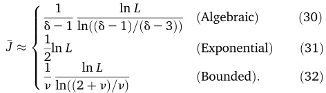
On matching the expectedfitnessFJ with theFJobtained in the above discussion for various distributions, we get
J
8 > > > > > < > > > > > :
1 d21
lnL
lnððd21Þ=ðd23ÞÞ ðAlgebraicÞ ð30Þ 1
2lnL ðExponentialÞ ð31Þ
1 n
lnL
lnðð2þnÞ=nÞ ðBoundedÞ: ð32Þ
Thus the above argument shows that for largeL,
JalnL; (33)
where the prefactor a depends on p(f). We note that aalgebraic,aexponential,abounded, which implies that smaller numbers of substitutions occur for fat-tailedfitness distribu-tions than for the bounded ones. To understand this quali-tative trend, consider the transition probability for thefirst step given byT(f)0)p(f)fp(f). At largef, this probability is higher for slowly decaying distributions and thus a large fitness gain occurs initially. But as the probability to exceed the highfitness achieved at thefirst step is small, the walk terminates sooner for broad distributions.
The results of our numerical simulations forJ shown in Figure 2 are in agreement with the logarithmic dependence onLbut the value of the prefactor does not match with that obtained above [except for p(f) =e2f]. The prefactor a is expected to interpolate between the two limiting cases of adaptive walks, namely greedy walk in which the best mu-tant is chosen with probability one and random adaptive walk in which all better mutants are chosen with equal probability. The former limit is obtained when d / 1 in (1) and the latter when n/ 0 in (3) (Joyceet al.2008).
Since the average walk length for a greedy walker is afinite constant equal toe211.718 for infinitely long sequences (Orr 2003), the prefactora= 0 whilea= 1 for the random adaptive walk (see Appendix A). In the following sections, wefind thata=1
2for exponentially distributedfitness and a =2
3 for the uniform case, which are consistent with the results in Figure 2 and the analytical results of Neidhart and Krug (2011), which are obtained using a simpler version of the adaptive walk model considered here.
Fitness distribution at thefirst step for general distributions
If the whole population is assumed to have an initialfitness f0, using P0(f) =d(f2f0) in (7) we have
P1ðfÞ ¼
ðf2f0ÞpðfÞ
12qLðf 0Þ
Ru
f0dgðg 2f0ÞpðgÞ
}ðf2f0ÞpðfÞ: (34)
The above fitness distribution at the first step is nonmono-tonic for all fitness distributions in (1–3) except for trun-cated distributions with n # 1. The implications of this result are examined in theDiscussion.
Entire walk with exponentially distributedfitness For p(f) =e2f, from (11) we obtain
~
P99Jþ1ðfÞ ¼
12qLðfÞ~PJðfÞ; J$1; (35)
whereq(f) = 12e2f. Due to (12) and (13), the boundary conditions arePJ(0) = 0 andPJ9ð0Þ ¼dJ;1.
We define a generating function
Gðx;fÞ ¼PNJ¼1~PJðfÞxJ; x,1;which obeys the following sec-ond-order ordinary differential equation:
G$ðx;fÞ ¼x12qLðfÞGðx;fÞ: (36)
To arrive at the above equation, we have used that ~
P1ðfÞ ¼f; which is obtained by using the initial condition in (7). The generating functionG(x,f) obeys a Schrödinger equation for the wave function of a particle in a one-dimen-sional potentialV(f)12qL(f) and energy zero (Mathews and Walker 2004). Since 12qLðfÞ 12e2Le2f is close to unity for f> lnLand vanishes forf ?ln L, the potential V(f) decreases smoothly from one to zero and moves right-ward with increasing L. Similar potentials also arise when two materials with different transport properties are joined together and in such systems, an analytical solution is obtained within a step function potential approximation (Blonder et al. 1982;Schaeybroeck and Lazarides 2009).
We follow this approach here and approximate the distribu-tion 1 2 qL(f) by the Heaviside theta function Qð~f2fÞ, where~f¼lnL. Within thisstep distribution approximation, we have
G$ðx;fÞ ¼
xGðx;fÞ; f,~f
0; f.~f: (37)
Forf,~f, the differential Equation 37 has a solution of the form G,ðx;fÞ ¼aþepffiffixfþa
2e2
ffiffi x pf
; which reduces to
G,ðx;fÞ ¼c sinhðpffiffiffixfÞ sinceG(x, 0) = 0 due to PJð0Þ ¼0. Since the solution forf,~f cannot depend on~f;we appeal to the infinite sequence length limit to fix the proportionality constantc. As noted earlier, the distributionPJ|L/N= 1 for allJ$0, which implies that
Z N
0
df e2fG,ðx;fÞ ¼ x
12x (38)
and therefore
G,ðx;fÞ ¼pxffiffiffisinh ffiffiffipxf: (39)
We check that the boundary condition PJ9ð0Þ ¼P~J9ð0Þ ¼dJ;1;
which is equivalent to G9(x,0) = x, is also satisfied by the above solution.
Forf.~f, the solutionG.(x,f) =af+b, where the
con-stants of integration a,bcan befixed by matching the solu-tionsG,andG.and theirfirst derivative atf¼~f. Thus the
constantsaandbare determined by the following conditions:
G,x;~f¼G.x;~f¼a~fþb (40)
G9,ðx;fÞjf¼~f ¼G9.ðx;fÞjf¼~f ¼a: (41)
A simple algebra shows that
G.ðx;fÞ ¼xcosh ffiffiffipx~ff2~fþpffiffiffixsinh ffiffiffipx~f: (42)
Using the above expressions forG(x,f), thefitness distri-butionPJ(f) for thefixed beneficial mutations can be calcu-lated. On expanding (39) and (42) in a power series about x= 0 and picking the coefficient ofxJ, we have
PJðfÞ ¼
e2ff2J21
ð2J21Þ!·
(
1; r#1
ð2J21Þr2ð2J22Þ
r2J21 ; r.1;
(43)
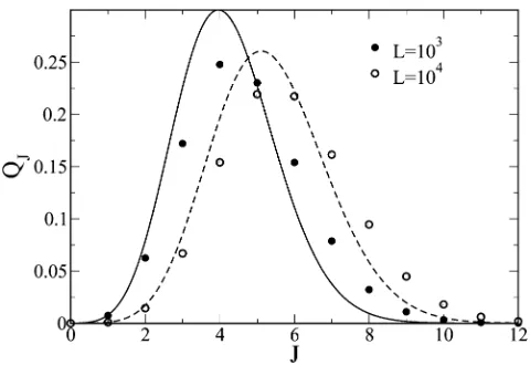
wherer¼f=~f. Figure 3 shows our numerical results forPJ(f) for the first few adaptive steps. As the walk proceeds, the distribution moves rightward as expected and its amplitude decreases since the probabilityqL(f) that the walker cannotfind a better neighbor approaches unity with increasing f. Our analytical result (43) is also shown in Figure 3 for compar-ison. ForL= 103, the step distribution approximation used tofind (43) gives 12qL(f)1 forf,lnL= 6.9 and zero otherwise. However, as the probability 12qL(f) stays close to unity forf#5 and decreases gradually to zero whenf 12, the distribution (43) in the region 5,f,12 does not match well with the simulation results but outside this crossover region, we see a good quantitative agreement. We also note that the fitness distribution does not move appreciably for J $ 4 and is centered aroundf 7 (see inset in Figure 3). This is because the average walk length forL= 103is4:6 steps (refer to Figure 2) and as the local optimum is approached, the fitness distribution of fixed beneficial mutation remains centered close to the typical fitness of the local optimum given by (26), which is lnL 6.9. This also explains the initial linear rise in the average fitness followed by a slower increase in Figure 1.
We next calculate the walk length distributionQJdefined by (17). Since qLðfÞ ¼Qðf2~fÞ within the step distribution approximation discussed above, (17) reduces to
QJ¼ Z N
~ f
df PJðfÞ: (44)
On integratingPJ(f) given in (43), we get
QJ¼e2lnL "
ðlnLÞ2J22 ð2J22Þ!þ
ðlnLÞ2J21 ð2J21Þ!
#
; J.0: (45)
Figure 3 Comparison of the distributionPJ(f) forJ¼1, 2, 3, 5 obtained numerically (points) and analytically (lines) given by (43) for exponentially distributedfitness and sequence lengthL¼1000. Inset: Numerical data forPJ(f) forJ¼4, 5, 6 to show that thefitness distribution does not shift appreciably beyondJ4:6as the local optimum with averagefitness7 is approached.
This expression is compared with numerical results in Figure 4 and shows a reasonable agreement. The average number of adaptive steps calculated using (45) is given by
J¼X
N
J¼1
JQJ
1
2lnL; (46)
which is in good agreement with the simulation result in Figure 2. The width of the distribution QJmeasured using the variances2¼J22J2lnL=4 also increases withL. Entire walk with uniformly distributedfitness
For p(f) = 1, since PJðfÞ ¼~PJðfÞ, the differential equation (11) reduces to
PJ99þ1ðfÞ ¼ 12f L R1
fdgðg2fÞ
PJðfÞ ¼
2
12fL
ð12fÞ2 PJðfÞ; J$1 (47)
with boundary conditions PJ(0) = 0 and PJ9ð0Þ ¼2dJ;1.
As before, we define a generating function
Gðx;fÞ ¼PNJ¼2xJ22PJðfÞ that obeys the second-order ordi-nary differential equation
G$ðx;fÞ ¼
212fL
ð12fÞ2 ðxGðx;fÞ þ2fÞ; (48)
where we have used thatP1(f) = 2f. We treat this case also within the step distribution approximation discussed earlier. Since the probability 12fL12e2L(12f), we approximate it by a step function Qð~f2fÞ, where ~f ¼ ðL21Þ=L. Forf,~f, we obtain an inhomogeneous second-order ordinary differ-ential equation with variable coefficients:
G,99ðx;fÞ ¼ 2x
ð12fÞ2G,ðx;fÞ þ 4f
ð12fÞ2: (49)
This equation can be solved by standard methods (detailed inAppendix C) to yield
G,ðx;fÞ ¼aþð12fÞaþþa
2ð12fÞa2þuþðfÞð12fÞaþ
þ u2ðfÞð12fÞa2; (50)
where the exponents
a6¼16
ffiffiffiffiffiffiffiffiffiffiffiffiffiffi
1þ8x p
2 : (51)
Thefirst two terms on the right-hand side give the solution of the homogeneous equation and the last two terms are the particular integral involving the variational parametersu6ðfÞ
given inAppendix C. The constants of integrationa6can be
obtained using the boundary conditions G(x, 0) = 0 and
R1
0df G,ðx;fÞ ¼ ð12xÞ2 1
. After some straightforward alge-bra, wefind that
G,ðx;fÞ ¼ 22
x
ð12fÞaþ2ð12fÞa2 aþ2a2 þf
: (52)
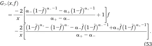
We verify that the condition PJ9ð0Þ ¼0 for J . 1 that amounts to G9(x, 0) = 0 is also satisfied. For f.~f, as G99.ðx; fÞ ¼0, the solution G.(x, f) = af + b, where a, bcan be determined using (40) and (41) to give
G.ðx;fÞ
¼2x2
"
a212~fa2212aþ12~faþ21
aþ2a2 þ1
#
f
22x "
12~faþ212~fa22a2~f12~fa221þaþf~12~faþ21
aþ2a2
# :
(53)
Explicit expressions forPJ(f) forfirst few adaptive steps are given inAppendix C and a comparison between the analyt-ical and the simulation results is shown in Figure 5.
Tofind the walk length distributionQJ ¼ R
~
f 1df P
JðfÞ, we define
Figure 5 Comparison of the distributionPJ(f) forJ¼1, 2, 3, 4 obtained numerically (points) and analytically (lines) given by (C6–C9) for uniformly distributedfitness and sequence lengthL¼100. The distribution forf#~f is shown in the main plot and forf.~f in the inset.
HðxÞ ¼ PN
J¼1
xJQJ
¼xQ1þx2 R
~
f1df G.ðx;fÞ
(54)
¼ x
12~f a22aþ
h
ð22aþÞ12~faþ2ð22a2Þ12~fa2
i : (55)
As an explicit expression forQJis rather unwieldy, its deri-vation and the expression itself are given inAppendix Cand a comparison with the simulations is shown in Figure 6. The average number of steps is given by
J¼dHðxÞ dx
x¼1¼
26ln12~f
9 ; (56)
which shows that for largeL, the number of adaptive steps grows as (2/3) lnLin agreement with the numerical results shown in Figure 2. The higher moments can also be found
straightforwardly and we find that the variance
J22J2 ð10=27ÞlnL and the skewness of the distribution decays slowly as (lnL)21/2.
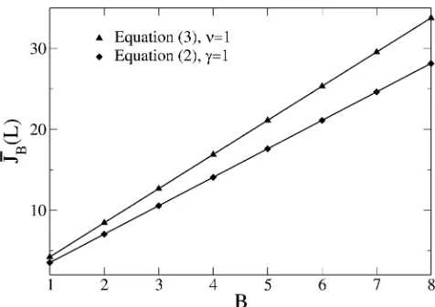
Effect of correlations on the number of adaptive steps We now turn to a discussion of adaptive walk properties when the fitnesses are correlated and given by a block model. We compute the average number JBðLÞ of adaptive steps given byPNJ¼1JQJðL;BÞ, where QJ(L,B) is the proba-bility that exactly J adaptive mutations occur when a se-quence of lengthLis divided intoBblocks.
Consider the distributionQ(m1,. . .,mB), which gives the joint probability that theith block of lengthLBin a sequence of lengthLcarriesmiadaptive mutations, wherei= 1,. . .,B. An important property of the block model is that this joint distribution factorizes; that is,
Qðm1; . . . ;mBÞ ¼ YB
b¼1
QmbðLB; 1Þ (57)
(Perelson and Macken 1995), where QJ(LB, 1)[ QJ(LB) is the walk length probability when thefitnesses are uncorre-lated and the sequence length is LB. The above equation expresses the fact that the block fitnesses evolve indepen-dently. As only one mutation occurs in the sequence at any step so that all but one block sequence remains unchanged and since the blockfitnesses are i.i.d. random variables, (57) holds.
Since the distributionQJ(L,B) is given by
QJðL; BÞ ¼ XJ
m1; ...;mB¼0
Qðm1; . . . ;mBÞdðm1þ. . . þmB2JÞ;
(58)
it follows that
JBðLÞ ¼X
N
J¼1
JX
J
mB¼0 QmBðLBÞ
X J2mB
m1;...;mB21¼0
Y B21
b¼1
QmbðLBÞ
· d X
B21
b¼1
mb2ðJ2mBÞ !
¼XN
J¼1
JX
J
mB¼0
QmBðLBÞQJ2mBðL2LB;B21Þ
¼XN
m¼0
QmðL2LB;B21Þ XN
n¼0ð
nþmÞQnðLBÞ
¼JðLBÞ þ XN
m¼1
mQmðL2LB;B21Þ
¼JðLBÞ þJB21ðL2LBÞ
¼BJðLBÞ;
(59)
where we have used that PNJ¼0QJðL;BÞ ¼1 and J is the average number of steps in the adaptive walk for uncorre-latedfitnesses. Figure 7 shows the results of our numerical simulations for average walk length when the block length LB=L/Bis keptfixed and the blockfitnesses are exponen-tially and uniformly distributed. For fixedLB, (59) predicts thatJBincreases linearly withB, which is in excellent agree-ment with the numerical data.
For largeL, due to (33) we have
JBðLÞ aB ln
L
B: (60)
For smallB, a linear rise in the average number of steps with the number of blocks has been seen numerically for expo-nential-like distributions and it was inferred that the mean walk length is independent of underlying fitness distribu-tions (Orr 2006). However, as discussed in the previous sections, the average number J depends on the fitness distribution p(f) and therefore the average JB is also nonuniversal.
Figure 7 Average numberJBof adaptive steps as a function of block
Discussion
In the last few years, several analytical results have been obtained for the mutational landscape model (Gillespie 1991). However, many of these results deal with thefirst step in the adaptation process (Orr 2002, 2006; Joyceet al.2008) and an extension of the theory to full adaptive walk is nec-essary. Previous studies also assume that the process of adap-tation starts from a highlyfit sequence that is not applicable to situations in which the population is subjected to high stress and hence has a very low initialfitness (MacLean and Buckling 2009; McDonaldet al.2010). In this article, we have obtained results for the entire adaptive walk starting from a low initialfitness but as discussed below, we expect some of these results to hold for moderately high initialfitness also.
Walk length distribution and average walk length
In previous works, the walk length distributions for the greedy walk and the random adaptive walk have been studied and found to be universal in that they are in-dependent of the underlying fitness distribution p(f). The origin of this universality property is clear in the light of the results of Joyceet al.(2008) who pointed out that these two models can be obtained as a limit of (4), which defines the mutational landscape model. For the random adaptive walk, the distribution QJ for infinitely long sequence van-ishes (see Equation A3) and the average walk length diverges with sequence length. In contrast, for the greedy walk, the walk length distribution in the L / N limit decreases exponentially fast with J for the greedy walk as a result of which the average number of steps turns out to be a constant (Orr 2003; Rosenberg 2005).
In this article, we have calculated the walk length distribution for exponentially and uniformly distributed fitnesses and found the average walk length for general fitness distributions. An important conclusion of our study is that the average number of adaptive steps increases logarithmically with the sequence length with a prefactor smaller than unity if the walk starts from zerofitness. Our simulations (not shown) also indicate that if the initial rank is of orderL, the average number of steps increases logarith-mically with the rank and with the same proportionality constant as that for the zero initial fitness case. Thus for a wild-type sequence with initial rank (or L) of the order 100, the number of substitutions is expected to be less than five. Although short adaptive walks have been observed in experiments (Rokyta et al. 2009; Schoustra et al. 2009), more detailed experimental studies testing the logarithmic dependence would be desirable. Although a test of the L dependence of the average walk length may not be experi-mentally viable, it should be possible to study the average walk length as a function of the initial rank.
Besides the sequence length, the number of steps to a local optimum depends on the underlying fitness distri-bution and thefitness correlations also. If the fitnesses are uncorrelated, as the numerical data in Figure 2 show, the
prefactor ain (33) depends on the shape of thefitness dis-tribution and therefore a rather detailed knowledge of the full fitness distribution (how fast it decays) is required to test this, which is presently unavailable. However, one can discern a trend in the value ofa: It decreases as thefitness distribu-tion broadens. This suggests that systems withfitness distri-bution in the Gumbel class (Imhof and Schlotterer 2001; Sanjuánet al.2004; Rokytaet al.2005; Kassen and Bataillon 2006; MacLean and Buckling 2009) will register shorter walks than those in the Weibull domain (Rokyta et al. 2008). As shown here in the block model of correlated fi t-nesses, the average number of adaptive steps increases as the number of blocks (and hencefitness correlations) increases. This is in accordance with the expectation that on a smooth correlated fitness landscape, as the local optima are less common (Perelson and Macken 1995), there is less chance to get trapped and therefore the uphill walk can last longer (Weinberger 1991; Kauffman 1993; Orr 2006).
Distribution offixed beneficial mutations during the walk
The fitness distribution PJ(f) has not been studied in pre-vious theoretical studies of adaptive walks in the SSWM limit and here we have computed this fitness distribution analytically using the recursion relation (7). Thefitness dis-tribution at thefirst step given by (34) can give a qualitative idea about the shape ofp(f). For mostfitness distributions, P1(f) is expected to be nonmonotonic but for bounded dis-tributions that diverge at the upper limit or the uniform distribution,P1(f) increases monotonically toward the upper bound. An inspection of the experimental data of Rokyta et al.(2005) shows thefitness distribution at thefirst step to be nonmonotonic, which is consistent with their assump-tion of exponentially decreasing distribuassump-tion of beneficial effects. It would be interesting to check whether the distri-butionP1(f) in Rokytaet al.(2008) is monotonic as the data in this study are consistent with a uniformly distributed
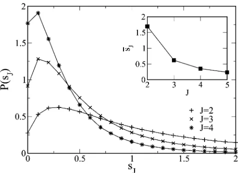
Figure 8 DistributionP(sJ) of selection coefficientsJforL¼1000 and
p(f)¼e2f. The inset shows the decay in average selection coefficient
fitness. The above behavior ofP1(f) is expected to be robust in the presence of correlations as at thefirst step in evolu-tion, the population has not sensed the correlations in the fitness landscape (Orr 2006).
For the fitness distribution for the entire walk, we presented an analysis for two distributions, namely expo-nential and uniform, that are consistent with the available experimental data. The distributionPJ(f) is obtained within a step distribution approximation that captures the shape of thefitness distribution correctly for thefirst few steps and leads to an accurate estimate of the number of average steps. Our approximation consists of replacing the probabil-ity 12qL(f) by a step functionQð~f2fÞ, where~f is given by (28) for exponentially and by (29) for uniformly distributed fitnesses. For f>~f and f?~f, our approximate solution matches the simulation results well for anyJ. With increas-ingJ, the distributionPJ(f) shifts toward higherfitnesses and peaks about~f for largerJ’s. As explained earlier, thefitness~f is reached whenJis close toJ
}lnLand therefore we expect our approximation to work well forJ>lnL.
When the underlying fitness distribution is exponential, we find that the fitness distribution of the fixed beneficial mutation also has an exponential tail (see Equation 43). The robustness of this result, i.e., whether any fitness distribu-tion in the Gumbel class exhibits an exponential tail for PJ(f), is, however, not clear. For uniformly distributed fi t-nesses, as the width of the distribution 1 2qL(f) decreases with increasingL, the step distribution approximation works better in this case than in the exponential case where the width is a constant (compare Figures 4 and 6). The proper-ties of multiple steps in an adaptive walk have been mea-sured in some recent experiments (Rokyta et al. 2009; Schoustraet al.2009) and a detailed analysis of the exper-imental results would be very welcome. On the theoretical front, an extension of the results described above to distri-butions other than uniform and exponential would be desir-able. We have recently made some progress in this direction and the results will appear elsewhere.
Another interesting question concerns the distribution P(sJ) of the selection coefficientsJ= (fJ2fJ21)/fJ21at the Jth step in the adaptive walk. As we start with zerofitness, the selection coefficient is defined forJ$2. Our preliminary numerical results forP(sJ) are shown in Figure 8 for thefirst few steps in the walk and we observe that the typical selec-tion coefficient decreases as the walk proceeds. This behav-ior matches qualitatively with the experimental results of Schoustra et al.(2009). A theoretical analysis of the distri-butionP(sJ) requires the joint distribution of thefitness at step J 21 and J and we hope to address this question in a future work.
Acknowledgments
K.J. thanks J. R. David for helpful suggestions and J. Krug for comments on an earlier version of the manuscript and useful correspondence. The authors also thank L. Wahl for
suggestions to improve the manuscript. K.J. thanks Kavli Institute of Theoretical Physics, Santa Barbara for hospitality and support under National Science Foundation grant PHY05-51164.
Literature Cited
Blonder, G. E., M. Tinkham, and T. M. Klapwijk, 1982 Transition from metallic to tunneling regimes in superconducting micro-constrictions: excess current, charge imbalance, and supercur-rent conversion. Phys. Rev. B 25: 4515.
Bull, J. J., and S. P. Otto, 2005 Thefirst steps in adaptive evolu-tion. Nat. Genet. 37: 342–343.
Carneiro, C., and D. Hartl, 2010 Adaptive landscapes and protein evolution. Proc. Natl. Acad. Sci. USA 107: 1747–1751. David, H., and H. Nagaraja, 2003 Order Statistics. Wiley, New York. Eyre-Walker, A., and P. Keightley, 2007 The distribution offitness
effects of new mutations. Nat. Rev. Genet. 8: 610.
Flyvbjerg, H., and B. Lautrup, 1992 Evolution in a ruggedfitness landscape. Phys. Rev. A 46: 6714–6723.
Gillespie, J. H., 1983 A simple stochastic gene substitution pro-cess. Theor. Popul. Biol. 23: 202–215.
Gillespie, J. H., 1991 The Causes of Molecular Evolution. Oxford University Press, Oxford.
Imhof, M., and C. Schlotterer, 2001 Fitness effects of advanta-geous mutations in evolving Escherichia coli populations. Proc. Natl. Acad. Sci. USA 98: 1113–1117.
Jain, K., 2011 Extreme value distributions for weakly correlated fitnesses in block model. J. Stat. Mech. 2011: P04020. Jain, K., A. Dasgupta, and G. Das, 2009 Exact and limit
distribu-tions of the largest fitness on correlated fitness landscapes. J. Stat. Mech. 2009: L10001.
Joyce, P., D. R. Rokyta, C. J. Beisel, and H. A. Orr, 2008 A general extreme value theory model for the adaptation of DNA sequen-ces under strong selection and weak mutation. Genetics 180: 1627–1643.
Kassen, R., and T. Bataillon, 2006 Distribution offitness effects among beneficial mutations before selection in experimental populations of bacteria. Nat. Genet. 38: 484–488.
Kauffman, S. A., 1993 The Origins of Order. Oxford University Press, New York.
Macken, C. A., and A. S. Perelson, 1989 Protein evolution on rugged landscapes. Proc. Natl. Acad. Sci. USA 86: 6191–6195. MacLean, R., and A. Buckling, 2009 The distribution offitness
effects of beneficial mutations in Pseudomonas aeruginosa. PLoS Genet. 5: e1000406.
Mathews, J., and R. L. Walker, 2004 Mathematical Methods of
Physics. Pearson Education, Delhi, India.
McDonald, M., T. F. Cooper, H. J. E. Beaumont, and P. B. Rainey, 2010 The distribution offitness effects of new beneficial mu-tations in Pseudomonasfluorescens. Biol. Lett. 7: 98–100. Miller, C. R., P. Joyce, and H. Wichman, 2011 Mutational effects
and population dynamics during viral adaptation challenge cur-rent models. Genetics 187: 185–202.
Neidhart, J., and J. Krug, 2011 Adaptive walks and extreme value theory. Phys. Rev. Lett. (in press).
Orr, H., 2003 A minimum on the mean number of steps taken in adaptive walks. J. Theor. Biol. 220: 241–247.
Orr, H. A., 2002 The population genetics of adaptation: the adap-tation of DNA sequences. Evolution 56: 1317–1330.
Orr, H. A., 2006 The population genetics of adaptation on corre-latedfitness landscapes: the block model. Evolution 60: 1113. Perelson, A., and C. Macken, 1995 Protein evolution on partially
Rokyta, D., P. Joyce, S. Caudle, and H. Wichman, 2005 An em-pirical test of the mutational landscape model of adaptation using a single-stranded DNA virus. Nat. Genet. 37: 441–444. Rokyta, D., C. J. Beisel, P. Joyce, M. T. Ferris, C. L. Burch et al.,
2008 Beneficialfitness effects are not exponential for two vi-ruses. J. Mol. Evol. 69: 229.
Rokyta, D., Z. Abdo, and H. Wichman, 2009 The genetics of ad-aptation for eight microvirid bacteriophages. J. Mol. Evol. 69: 229.
Rosenberg, N., 2005 A sharp minimum on the mean number of steps taken in adaptive walks. J. Theor. Biol. 237: 17–22. Rozen, D., J. de Visser, and P. J. Gerrish, 2002 Fitness effects of
fixed beneficial mutations in microbial populations. Curr. Biol. 12: 1040–1045.
Sanjuán, R., A. Moya, and S. Elena, 2004 The distribution of fitness effects caused by single-nucleotide substitutions in an RNA virus. Proc. Natl. Acad. Sci. USA 101: 8396–8401. Schaeybroeck, B., and A. Lazarides, 2009 Normal-superfluid
in-terface for polarized fermion gases. Phys. Rev. A 79: 053612. Schoustra, S., T. Bataillon, D. Gifford, and R. Kassen, 2009 The
properties of adaptive walks in evolving populations of fungus. PLoS Biol. 7(11): e1000250.
Sornette, D., 2000 Critical Phenomena in Natural Sciences. Springer-Verlag, Berlin.
Weinberger, E. D., 1991 Local properties of Kauffman’s N-k model: a tunably rugged energy landscape. Phys. Rev. A 44: 6399–6413.
Communicating editor: L. M. Wahl
Appendix A: Random Adaptive Walk
In this Appendix, we briefly review the known results for random adaptive walk in which all better mutants are chosen with equal probability (Macken and Perelson 1989; Flyvbjerg and Lautrup 1992; Kauffman 1993). The probability distri-butionPJ(f) obeys the recursion relation
PJþ1ðfÞ ¼ Z f
l
dhRupðfÞ hdg pðgÞ
12qLðhÞPJðhÞ (A1)
(Flyvbjerg and Lautrup 1992), whereqðfÞ ¼Rfldg pðgÞ. A change of variable from thefitnessfto the cumulative probabilityq (f) gives
PJþ1ðqÞ ¼ Z q
0
dq912q9
L
12q9PJðq9Þ: (A2)
Since the walk length distribution for the random adaptive walk also obeys (17), we have
QJ¼ Z u
l
dh qLðhÞPJðhÞ ¼ Z u
l
dq qLPJðqÞ; (A3)
which shows thatQJis auniversal distributionin that it is independent of the underlyingfitness distributionp(f). Note that for infinitely long sequences, the probabilityQJ= 0 as in the mutational landscape model. Differentiating (62) with respect toqimmediately gives
dPJþ1ðqÞ
dq ¼
12qL
12qPJðqÞ ¼
XL
n¼0
qnPJðqÞ: (A4)
The generating functionGðx;qÞ ¼PNJ¼1xJPJðqÞthen obeys the followingfirst-orderdifferential equation:
G9ðx;qÞ2xP19ðqÞ ¼x12q L
12qGðx;qÞ: (A5)
For the initial conditionP0(f) =d(f), we haveP1(q) = 1 and due to (A2), the distribution PJ(0) = 0. Solving the above differential equation using these boundary conditions gives Gðx;qÞ ¼xexHLðqÞ, where H
LðqÞ ¼ PL
k¼1qk=k and hence the distributionPJ(q) is given by
PJðqÞ ¼H J21
L ðqÞ
ðJ21Þ! (A6)
(Flyvbjerg and Lautrup 1992). Since the productqLP
QJe2J
JJ21
ðJ21Þ!; (A7)
whereJ¼lnL. Thus the walk length distribution is a Poisson distribution (inJ) with meanJ¼lnL(Flyvbjerg and Lautrup 1992).
Appendix B: Simulation Procedure
For short sequences of lengthL#10 and uncorrelatedfitnesses, a randomly chosen sequence was assigned afitness equal to zero. Then the rest of the fitness landscape composed of 2L 2 1 fitnesses was generated by drawing random variables independently from a common distribution p(f). The transition probability from the initial sequence to each of the better sequences among theLnearest neighbors was calculated according to (4) and thefixed sequence at thefirst step in the adaptive walk was chosen. Then the transition probability from the chosen mutant sequence to its better neighbors was calculated and this process was repeated until afitter sequence was not available.
To simulate sequences with lengthL$102, we followed an approximate procedure outlined in Orr (2002) as the total number of sequences 2Lis prohibitively large for long sequences. Starting with zerofitness,Li.i.d. random variables were generated and a higherfitnessfwas chosen according to the transition probability (4). During the next step in the process,L new i.i.d. random variables were generated and the transition probability from fto a betterfitness was calculated. These steps were repeated until the new set of randomfitnesses did not exceed the currentlyfixedfitness. The block model was simulated to generate weakly correlated fitnesses by assigning independent fitnesses to each block sequence. In all the simulations, the data were collected using 106independent realizations of thefitness landscape.
Appendix C: Derivations for Uniformly Distributed Fitness
Solution of Differential Equation 49
The generating functionG,(x,f) obeys the inhomogeneous second-order differential equation
G$ðx;fÞ2 2x
ð12fÞ2Gðx;fÞ ¼ 4f
ð12fÞ2; (C1)
where we have dropped the subscript for brevity. The general solution of such differential equations is a linear combination of the general solution GH(x,f) of the homogeneous equation obtained by setting the right-hand side equal to zero and the particular solutionGPof the inhomogeneous equation (Mathews and Walker 2004). The homogeneous solution is of the form
GHðx;fÞ ¼aþð12fÞaþþa2ð12fÞa2; (C2)
wherea6are the solutions of the quadratic equationa22a22x= 0 and given by (51). The particular solution is found
using the method of variation of parameters and is of the formGPðx;fÞ ¼uþðxÞð12fÞaþþu2ðxÞð12fÞa2, where the functions u6(f) obey the followingfirst-order differential equations:
u9þðfÞð12fÞaþþu9
2ðfÞð12fÞa2¼0 (C3)
aþu9þðfÞð12fÞaþ21þa
2u92ðfÞð12fÞa221¼ 4f
ð12fÞ2 (C4)
(Mathews and Walker 2004). On solving the above equations, we obtain
GPðx;fÞ ¼ 4
aþa22
4ð12fÞ ð12aþÞð12a2Þ¼
22f
x : (C5)
Finally, using the boundary conditions in the general solutionG,(x,f) =GP(x,f) +GH(x,f), the desired result (Equation 52) is obtained.
Distribution of Fixed Beneficial Mutations
Thefitness distribution found using (52) and (53) is given below for thefirst few adaptive steps:
P2ðfÞ ¼ 8 < :
28fþ4ðf22Þlnð12fÞ; f#~f
4~ffþ~f22
12~f þ4ðf22Þln
12~f; f.~f (C7)
P3ðfÞ ¼4 8 > > < > > :
12fþlnð12fÞð1226fþflnð12fÞÞ; f#~f
1 12~f
6~f22f2~fþ26262~f~f2f322~fln12~f
þ f12~fln212~fi; f.~f
(C8)
P4ðfÞ ¼ 28
3
8 > > < > > :
120fþ60ð22fÞlnð12fÞ þ12fln2ð12fÞ þ ð22fÞln3ð12fÞ; f#~f 1
12~f
60~f22f2~fþ12f523~f225252~f~fln12~f
þ 3f223~fþ22~f~fln212~fþ ð22fÞ12~fln312~f; f.~f:
(C9)
Walk Length Distribution
On matching powers of xJon both sides in (55), we get
Q1¼e22ℓ
21þ2eℓ (C10)
Q2¼2e22ℓ
3þℓþ ð23þ2ℓÞeℓ (C11)
Q3¼e22ℓ
2218þ8ℓþℓ2þ4eℓ925ℓþℓ2 (C12)
Q4¼
4e22ℓ
3
180þ84ℓþ15ℓ2þℓ3þeℓ2180þ96ℓ221ℓ2þ2ℓ3; (C13)
whereℓ= lnL. A general solution ofQJby this method does not seem possible but an approximate analytic expression forQJ can be obtained as explained below.
From the definition of the generating functionH(x) in (55), it follows that
QJ¼
1 J!
dJHðxÞ
dxJ
x¼0: (C14)
By the residue theorem for complex variables, we have
1 2pi
Z
C
dz fðzÞ ¼ 1 n!
dn dznððz2z0Þ
nþ1
fðzÞÞ z¼z0
(C15)
(Mathews and Walker 2004), where z0 is a pole of order n + 1 of the function f(z) and the contour C encloses the singularities off(z). From (C14) and (C15), we can write
QJ¼ 1
2pi
Z
C
dzHðzÞ zJþ1 ¼
1 2pi
Z
C
dz eKðzÞ; (C16)
whereK(z) = lnH(z)2(J+ 1) lnz. We solve this integral by the method of steepest descent, which for largeJgives
QJ
ffiffiffiffiffiffiffiffiffiffiffiffiffiffiffiffiffiffiffiffi
1 2pK$ðzsÞ s
eKðzsÞ¼
ffiffiffiffiffiffiffiffiffiffiffiffiffiffiffiffiffiffiffiffi
1 2pK$ðzsÞ s
HðzsÞ
zJsþ1
(C17)
H9ðzsÞ
HðzsÞ ¼
J
zs (C18)
and
K$ðzsÞ ¼
H9ðzÞ HðzÞ
9
z¼zs
þ J
z2 s
(C19)
¼
H9ðzÞ HðzÞ
9
z¼zs
þ1 zs
H9ðzsÞ
HðzsÞ; (C20)
where the prime denotes a derivative with respect toz. Sincea+.0, neglecting the exponentially small term inð12~fÞaþ in (55), we get
HðzÞ e23ℓ=2eℓy=2ð3þyÞ
y221
16y ; (C21)
wherey¼pffiffiffiffiffiffiffiffiffiffiffiffiffiffi1þ8z. DifferentiatingH(z) once with respect tozgives
H9ðzÞ
HðzÞ
8ðyþ3Þ þ4ð2yþ3Þy221þ2yðyþ3Þy221ℓ
y2ðy221Þðyþ3Þ : (C22)
Using the above expression in (C18) for largey, we getys4J/ℓand therefore
zs2J 2
ℓ2 : (C23)
On differentiating (C22) once, we have
H9ðzÞ HðzÞ
9
4 y
"
4 3ðyþ3Þ2þ
4 ð1þyÞ22
4þ6ℓ 3y2 þ
8 y32
4 ð12yÞ2
#
: (C24)
Using (C22) and (C24) in (C20), we obtain
K$ðzsÞ
8
h
236þ6ys
y2s23
þysðysþ3Þ2ð1þysÞ2ℓ i
y4
sðysþ3Þ2
y2 s21
(C25)
8ℓ y3 s
¼ a4
8J3: (C26)
Thus we have
QJ
2J3=2 ffiffiffiffi
p p
ℓ2 ·
22a2ðzsÞ
aþðzsÞ2a2ðzsÞ ·
12~f1þa2ðzsÞ
zJ s
; (C27)