Methods for Interquantile Shrinkage and Variable Selection in Linear Regression Models.

ABSTRACT

JIANG, LIEWEN. Methods for Interquantile Shrinkage and Variable Selection in Linear Regression Models. (Under the direction of Huixia Wang and Howard Bondell.)

Conventional research on quantile regression often focuses on fitting the regression

model at different quantiles separately. However, in situations where the quantile

coeffi-cients share some common features, joint modeling of multiple quantiles to accommodate

the commonality often leads to more efficient estimation. One example of common

fea-tures is that a predictor may have a constant effect over one region of the quantile levels

but varying effects in other regions. To automatically perform estimation and detection of

the interquantile commonality, we develop two penalization methods. When the quantile

slope coefficients indeed do not change across quantile levels, the proposed methods will

shrink the slopes towards constant and thus improve the estimation efficiency.

Further-more, if the slope coefficients for some predictors are not significant at certain quantile

levels, or more extremely, over all quantile levels, additional penalization is included to

achieve the variable selection purpose. We establish the oracle properties of the proposed

methods. Through numerical investigations, we demonstrate that the proposed

meth-ods lead to estimations with competitive or higher efficiency than the standard quantile

©Copyright 2012 by Liewen Jiang

Methods for Interquantile Shrinkage and Variable Selection in Linear Regression Models

by Liewen Jiang

A dissertation submitted to the Graduate Faculty of North Carolina State University

in partial fulfillment of the requirements for the Degree of

Doctor of Philosophy

Statistics

Raleigh, North Carolina

2012

APPROVED BY:

Wenbin Lu Yichao Wu

Huixia Wang

Co-chair of Advisory Committee

Howard Bondell

DEDICATION

BIOGRAPHY

Liewen Jiang was born on July 3rd, 1985 in Shangyu, China. Shangyu is a beautiful

coastal city which lays on the mouth of the Hangzhou Wan River. In 2007, Ms. Jiang

graduated with a Bachelors degree in statistics from Sun Yat-sen University, Guangzhou,

China. Upon graduating from Sun Yat-sen University, Ms. Jiang was granted a full

schol-arship to North Carolina State University to earn her Doctorate in statistics. The focus

of Ms. Jiang’s research was directed on the interquantile shrinkage and variable selection

in linear quantile regression models. Along this academic journey, Ms. Jiang earned her

Master degree in 2009 and is expected to graduate with her Doctorate in the Summer of

2012.

During graduate school, Ms. Jiang had the opportunity to participate in two

sum-mer internships. In 2010, she spent three months in Burlington, Vermont at Precision

Bioassay Inc., where she worked closely with Dr. David Lansky and contributed herself

to developing the software package on analyzing bioassay data. The summer of 2011

of-fered Ms. Jiang an incredible internship at Amgen Inc. located in Seattle, Washington.

She worked on mining historical rat data to predict liver toxicity. During this internship,

she maintained close collaborations with toxicologists and biostatisticians, and received

ACKNOWLEDGEMENTS

First and foremost, I would like to express my deep appreciation to my advisors Dr. Huixia

(Judy) Wang and Dr. Howard Bondell. Without their patient and effective guidance,

this thesis would not exist. I would also like to thank my committee memebers: Dr.s

Wenbin Lu, Yichao Wu and Khaled Harfoush. Their valuable advices and comments

helped strengthen this thesis. I also want to thank our fantastic Directors of Graduate

Program (GDPs) in the department of statistics: Dr.s Sujit K. Ghosh, John Monahan,

Pam Arroway, and Jacqueline Hughes-Oliver, for helping me out during my stay in the

graduate program.

My appreciation also goes to Dr. David Lansky, my supervisor at Precision Bioassay

Inc., and Dr.s Cheng Su and Yudong He, my mentors at Amgen Inc. They offered me

great opportunities to gain some valuable industrial experience even before I start my

career.

I would also like to thank all my friends. We shared many great moments in the

graduate school, and with their supports and encouragements, I was able to go through

many difficult situations. I certainly hope that we can maintain close friendship in the

future.

Last but not the least, I would like to show my deepest appreciation to my parents.

Without their endless love and support, I would never get to this stage. Being their child

TABLE OF CONTENTS

List of Tables . . . vii

List of Figures . . . ix

Chapter 1 Introduction . . . 1

1.1 Quantile Regression . . . 1

1.2 Hypothesis Tests in Quantile Regression . . . 4

1.3 Variable Selection . . . 6

Chapter 2 Interquantile Shrinkage in Regression Models . . . 12

2.1 Introduction . . . 12

2.2 Proposed Method . . . 15

2.2.1 Model Setup . . . 15

2.2.2 Penalized Joint Quantile Estimators . . . 17

2.2.3 Computations . . . 18

2.3 Asymptotic Properties . . . 19

2.3.1 Fused Adaptive LASSO Estimator . . . 20

2.3.2 Fused Adaptive Sup-norm Estimator . . . 21

2.4 Simulation Study . . . 22

2.4.1 The Comparison of Different Group-wise Weights in FAS . . . 29

2.5 Real Data Study . . . 33

2.6 Theoretical Proof . . . 40

Chapter 3 Non-crossing Quantile Estimation . . . 47

3.1 Introduction . . . 47

3.2 Non-crossing Constraints . . . 48

3.3 Simulation Studies . . . 50

3.4 Real Data Revisited . . . 52

Chapter 4 Variable Selection in Joint Quantile Regression Models . . . 55

4.1 Introduction . . . 55

4.2 FAL Variable Selection Estimator . . . 57

4.2.1 Proposed Method . . . 57

4.2.2 Oracle Estimator . . . 58

4.2.3 VFAL Estimator . . . 60

4.3 FAS Variable Selection Estimator . . . 60

4.4 Computations . . . 63

4.5 Simulation Study . . . 65

4.7 Theoretical Proof . . . 75

Chapter 5 Discussions and Future Work . . . 81

5.1 Weighted Loss Function . . . 82

5.2 Nonparametric Quantile Regression . . . 84

LIST OF TABLES

Table 2.1 The MISE and ORACLE proportions of different methods in Ex-ample 2.1. . . 24 Table 2.2 Percentage of correctly identifying dk = β(τk)−β(τk−1) over 500

simulations in Examples 2.1-2.3. . . 27 Table 2.3 The MISE and ORACLE proportion of different methods in

Exam-ple 2.4 withγ = 2 and γ = 0, respectively. . . 28 Table 2.4 True Proportion of True Positive (TP) for each interquantile

differ-encedk,l in Example 2.4 withγ = 2 andγ = 0, respectively. The

in-terquantile slope differencesdk,l =βk,l−βk−1,l, l= 1,2, k = 2, . . . ,9.

For γ = 2, the true coefficients dk,1 = 0, but dk,2 6= 0 for all k. For γ = 0, dk,l = 0 for all k and l. . . 29

Table 2.5 The MISE and ORACLE of FAS by adopting different group-wise weights in Example 2.4 with γ = 0 andγ = 2, respectively. . . 32 Table 2.6 Estimated quantile slope coefficients for economic growth data by

FAL. The tuning parameter is selected by AIC. Neighboring esti-mates with underlines beneath are identical. . . 36 Table 2.7 Estimated quantile slope coefficients for economic growth data by

FAS. The tuning parameter is selected by BIC. Neighboring esti-mates with underlines beneath are identical. . . 37

Table 3.1 100×MISE (100×s.e.) of FAL and FAS without and with noncross-ing constraints in Example 3.1 with p = 2 and γ = 2, where the quantile slope coefficients for the 1st predictor are constant, but vary across quantiles for the 2nd predictor. . . 52 Table 3.2 100×MISE (100×s.e.) of FAL and FAS with and without

noncross-ing constraint in Example 3.2 with p = 6, where the slope coeffi-cients corresponding tox3. . . x6 vary across quantiles, but the slope coefficients forx1 and x2 are constant. . . 53 Table 3.3 Average prediction errors with and without non-crossing constraints

for economic growth data. The values in the paretheses are standard errors. . . 53

Table 4.1 The performance of VAL, VFAL, VAS and VFAS methods in 6-dimensional case, where β6(τ) = 2 + Φ−1(τ) vary with τ, β3(τ) = β4(τ) = β5(τ) = 0, and β1(τ) =β2(τ) = 1. . . 69 Table 4.2 MISE of VAL, VFAL, VAS and VFAS methods in 6-dimensional case

Table 4.3 Estimated quantile slope coefficients for economic growth data by using VFAL and VFAS methods, respectively. The tuning parameter is selected by AIC. . . 72 Table 4.4 Estimated quantile slope coefficients for economic growth data by

using VFAL and VFAS methods. The tuning parameter is selected by BIC. . . 73 Table 4.5 Prediction Errors (PE) by using both VFAL and VFAS methods

LIST OF FIGURES

Figure 2.1 Estimated quantile coefficients for the first 9 covariates (intercept is not included) from RQ (solid line), FAL (dashed line with dots) and FAS (dashed line with stars). X-axis is quantile levels. Shaded areas are the 90% pointwise confidence bands from the inverse rank method. . . 38 Figure 2.2 Estimated quantile coefficients for the rest 4 covariates (intercept

is not included) from RQ (solid line), FAL (dashed line with dots) and FAS (dashed line with stars). X-axis is quantile levels. Shaded areas are the 90% pointwise confidence bands from the inverse rank method. . . 39

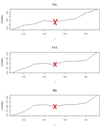
Figure 3.1 Estimated conditional quantiles of GDP growth given the predic-tors having the same characteristics as the ones for Zimbabwe in period 1965-75. The upper plot is for unconstrained FAL, the mid-dle one is for unconstrained FAS, and the lower one is for uncon-strained RQ. Y-axis is the estimated quantiles. Specially, the 0.4th conditional quantile is estimated larger than the 0.5th _{quantile for}

all the three methods, indicating that the unconstrained FAL, FAS and RQ methods suffer from the quantile crossing issue. . . 54

Chapter 1

Introduction

1.1

Quantile Regression

Regression is a core method in statistics. Traditional regression analysis focuses on the

mean, which explores the impact of explanatory variables (predictors) on the mean of

the dependent variable (response). A standard approach in estimating the mean

regres-sion function is Ordinary Least Squares (OLS), in which the unknown parameters are

estimated by minimizing the sum of squared errors. More explicitly, consider a linear

regression model

yi =xiTβ+i, i= 1. . . n,

where β= (β1, . . . , βp)T ∈Rp, xi ∈Rp is the design vector and {i}ni=1 are independent random errors with mean zero. The OLS estimate of β is obtained by minimizing

n

X

i=1

(yi−xiTβ)2.

real applications, heavy-tailed response distributions frequently occur, making the

condi-tional mean regression unstable because it is highly influenced by outliers. An alternative

method is the median regression, which describes the central location of the response

dis-tribution, and is robust to outliers. The Least Absolute Deviation (LAD) method, which

minimizes the sum of absolute errors

n

X

i=1

|yi−xiTβ|,

is used to estimate the conditional median regression function. Secondly, the conditional

mean regression can not provide information about the tail behaviors of the response

distribution without strict parametric assumptions. For instance, the tax-policy study

focuses more on the rich, say, the top 4% of the population, instead of on the mean [27].

Koenker and Bassett (1978) [15] introduced Quantile Regression (QR), a valuable

al-ternative to the ordinary least squares. Quantile regression can automatically capture the

change in any conditional quantile of the response associated with the change in

covari-ates. Therefore, it is more flexible for assessing the relationship between the predictors

and the response. Consider a linear quantile regression model

yi =xTi β(τ) +i,

where i are independent random errors whose τth conditional quantile given xi equals

zero. The τth linear conditional quantile regression model is

Qτ(x) = xTβ(τ), (1.1)

estimate the conditional mean regression function, the τth _{conditional quantile function}

can be estimated by minimizing the sum of asymmetric absolute errors

n

X

i=1

ρτ(yi−xiTβ), (1.2)

where ρτ(u) = u(τ −I(u < 0)) is the so-called check function. At τ = 0.5, the quantile

regression reduces to the least absolute deviation regression.

Quantile regression has attracted enormous attention in various areas since its

in-troduction. Successful applications of quantile regression include the studies of market

returns [3] , risk modeling [6], survival outcomes [17], agricultural land prices [20],

pollu-tion data [23], growth chart [33], microarray data [31], and so forth.

In general, regression at multiple quantiles provides more comprehensive statistical

views than single quantile regression. The standard approach of regression at multiple

quantiles is to fit the quantile regression model at each quantile separately. However, in

applications where the quantile coefficients enjoy some common features across

quan-tile levels, joint modeling at multiple quanquan-tiles can lead to more efficient estimation as

illustrated in Zou and Yuan (2008)[42]. One special case is the regression model with

in-dependent and identically distributed (i.i.d.) errors so that the quantile slope coefficients are constant across all quantile levels. Under this assumption, Zou and Yuan (2008)[40]

proposed the Composite Quantile Regression (CQR) method by combining the objective

functions at multiple quantiles to estimate the common slopes. They showed that for

models withi.i.d. errors, the composite estimator is more efficient than the conventional estimator obtained at a single quantile level. However, in practice, thei.i.d.error assump-tion is restrictive and needs to be verified. It is likely that the quantile slope coefficients

model at multiple quantiles, the common structure of quantile slopes has to be

deter-mined. One way to identify the commonality of quantile slopes at multiple quantile levels

is through hypothesis testing. In Section 1.2, we describe the Wald-type test based on

direct estimation of the asymptotic covariance matrix of quantile coefficient estimates at

multiple quantiles.

1.2

Hypothesis Tests in Quantile Regression

Suppose we are interested inKconditional quantile functions with quantile levelsτ1, . . . , τK.

Assume the linear quantile regression model (1.2), we consider a general linear hypothesis

H0 :Rβ=γ,

where β = (βT(τ1), . . . ,βT(τk))T is a pK×1 parameter vector of quantile slope

coeffi-cients andβ(τj)∈Rp forj = 1, . . . , K. The pre-specifiedq×(pK) matrixRhas full rows,

and γ is a q×1 hypothetical vector. For example, suppose we are interested in testing the equality of quantile slopes across quantile levels τ1, . . . , τK, that is, testing the null

hypothesis H0 : β(τ1) = β(τ2) = . . .= β(τK), it is equivalent to testing H0 :Rβ = γq,

where

R=         

Ip −Ip 0 0 . . . 0

0 Ip −Ip 0 . . . 0

.. .

0 0 . . . 0 Ip −Ip

         ,

The Wald-type test statistic is constructed as

Tn =n(Rβˆ −γ)T(RVnRT)−1(Rβˆ −γ),

Koenker and Bassett (1982)[16] have shown that under H0, the test statistic Tn

asymp-totically follows χ2

q distribution. Here, Vn is the pK×pK asymptotic covariance matrix

of √nβˆ. Specifically, Vn= (Vn(i, j), i, j = 1, . . . , pK) has the sandwich form [9], with

Vn(i, j) = (τi∧τj −τiτj)Hn(τi)−1JnHn(τj)−1,

where

Jn=n−1 n

X

i=1

xixiT

and

Hn(τ) = lim n→∞n

−1

n

X

i=1

xixiTfi{ξi(τ)},

where ξi(τ) = xTiβ(τ) is the τth conditional quantile of yi given xi and fi{ξi(τ)} is the

conditional density of yi, evaluated at the τth conditional quantile ξi(τ) [9].

There are several approaches proposed to estimate the matrix Hn. Hendrickes and

Koenker (1991)[8] showed that by assuming the τth conditional quantile function of y given xis linear fort ∈[τ−hn, τ +hn], the parameters β(τ+hn) andβ(τ−hn) can be

consistently estimated, and the density fi{ξi(τ)} in Hn(τ) can be estimated by

ˆ

fi{ξi(τ)}=

2hn xT

i {βˆ(τ+hn)−βˆ(τ−hn)}

.

A potential problem is that the estimated conditional quantiles may cross, that is,

xT

the estimated density function ˆfi{ξi(τ)}is not guaranteed. Hendricks and Koenker(1991)

[8] suggested

ˆ

f_i+ = max

0, 2hn di−

to replace the estimate ˆfi, where di =xTi {βˆ(τ +hn)−βˆ(τ−hn)}, and >0 is a small

tolerance parameter with the purpose of avoiding zero denominators in some special

cases.

Powell et al. (1991)[25] proposed an alternative kernel estimation approach to

ap-proximate the matrix Hn, formulated as

ˆ

Hn(τ) = (nhn)−1

X

i

KN{ˆui(τ)/hn}xixTi ,

where ˆui(τ) = yi−xTi βˆ(τ),hnis the bandwidth satisfyinghn →0 andn1/2hn → ∞. The

notation KN(·) is for the kernel function. If the bandwidth hn and the kernel function

KN(·) are chosen appropriately, under certain conditions, Powell et al. (1991)[25] shows that ˆHn(τ)−Hn(τ)→0 in probability.

1.3

Variable Selection

Variable selection is very important in model building. In practice, it is common to

in-clude a large number of predictors at the initial stage of modeling in order to attenuate

the possible estimation biases. However, keeping too many predictors, especially the

irrel-evant ones in the model will make the interpretation difficult and decrease the prediction

accuracy. Hence, it is desirable to select simpler models containing only important

pre-dictors.

selection is a classic variable selection method. However, subset selection is a discrete

process with predictors being either in or out of the model, which lacks theoretical

prop-erties and model stability. It is possible that a small change in data will result in a very

different model by using subset selection.

As a remedy, penalization has become a popular tool for automatic estimation and

variable selection over the past decades, as it enjoys the favorable properties of both

subset selection and ridge regression. Various penalization methods have been introduced

in the literature for different selection purposes. For example, Least Absolute Shrinkage

and Selection Operator (LASSO), proposed by Tibshirani (1996)[29], penalizes the sum

of absolute values of the coefficients (L1-penalty). Specifically, the lasso estimate ˆβ_LASSO

is defined by

ˆ

β_LASSO = arg min

β

n

X

i=1

(yi−xTi β)

2_+λ

p

X

j=1 |βj|,

where λ ≥ 0 is a tuning parameter that controls the degree of shrinkage. If λ is large enough, all slopes βj for j = 1. . . p will be shrunk to exactly 0. On the other hand, if

λ= 0, no shrinkage will be imposed on the coefficients and the LASSO estimator reduces to ordinary least squares estimator.

Fan and Li (2001)[5] proposed another penalization method called the Smoothly

Clipped Absolute Deviation (SCAD), which is a nonconcave penalty and defined through

its first order derivative. The SCAD estimate ˆβ_SCAD is defined as

ˆ

β_SCAD = arg min

β

n

X

i=1

(yi−xTi β)

2 +

p

X

j=1

pλ(βj),

where p0_λ(βj) = λ{I(βj ≤ λ) +

(aλ−βj)+

(a−1)λ I(βj > λ)} is the first order derivative of pλ(βj),

that SCAD estimator enjoys the following good properties:

(i) unbiasedness: when the true unknown parameter is large, the corresponding

esti-mator is nearly unbiased;

(ii) sparsity: the small estimated coefficients are automatically set to zero in order to

improve model interpretability;

(iii) continuity: the resulting estimator is continuous to avoid model instability.

Zou (2006)[39] proposed the Adaptive LASSO (ALASSO) penalization method by

including adaptive weights in the L1-penalty. The ALASSO estimate ˆβ_ALASSO is defined by

ˆ

β_ALASSO = arg min

β

n

X

i=1

(yi−xTi β)

2_+λ

p

X

j=1 ˜ wj|βj|,

where ˜wj are adaptive weights controlling the shrinkage speeds for various components

βj, j = 1, . . . , p. If the weights are selected appropriately, for example, let ˜wj = (|β˜j|)−r,

where ˜βj are some consistent initial estimators and r > 0 is a constant, the adaptive

LASSO estimator possesses the oracle properties.

In some circumstances, instead of selecting individual variables, we might be interested

in selecting important explanatory factors, each of which consists of a group of input

varibles. For example, in the multifactor analysis-of-variance (ANOVA), each factor tends

to have several levels, which can be expressed by a group of dummy variables. Thus,

selecting the main effects and interactions essentially becomes selecting the important

groups of variables (factors). Suppose we consider a regression model with J factors

Y =

J

X

j=1

Xjβj+,

where Y ∈Rn,β_j = (βj1, . . . , βjpj)

T _{is ap}

and ∈Rn. To select variables Xj with zero βj, Yuan and Lin (2006)[36] proposed the

Group LASSO (GLASSO) penalized estimator

ˆ

β_GLASSO = arg min

β kY −

J

X

j=1

Xjβjk

2_+λ

J

X

j=1

kβ_jkKj,

wherek·k2 _{is theL}

2-norm, andkβjkKj = (β

T

jKjβj)1/2, provided that the kernel matrices K1 ∈ Rpj×pj, . . . ,KJ ∈ Rpj×pj are positive definite matrices. In GLASSO, the penalty

function is between the L1-penalty in LASSO andL2-penalty in ridge regression. Hence, it encourages the sparsity in factors, but not in individual variables.

For selecting important factors in classification problems, Zou and Yuan (2008)[41]

proposed a F∞-norm penalization, where the penalty function becomes

J

X

j=1

kβ_jk∞ =

J

X

j=1

max{|βj1|, . . . ,|βjpj|}.

When pj = 1 for all j, the F∞ reduces to the L1-penalty. Unlike LASSO penalty that leads to selection of individual variables,F∞-norm encourages groupwise selection. If the parameter λ is chosen appropriately, some β_j will be shrunk to exactly zero as a whole group, that is, βj1 =. . .=βjpj = 0 for some j.

The aforementioned penalization methods are used for selecting important variables

or factors to achieve sparse models. Some other penalization approaches are designed for

smoothing and selecting variables simultaneously. Tibshirani et al. (2005)[30] introduced

Fused LASSO (FLASSO) approach, which penalizes theL1-norm of both the coefficients and their successive differences. The FLASSO estimator is defined as

ˆ

β_FLASSO = arg min

β

n

X

i=1

(yi−xTiβ)

2 +λ1

p

X

j=1

|βj|+λ2 p

X

j=2

where λ1 ≥ 0 and λ2 ≥ 0 are two tuning parameters controlling the sparsity and the smoothness of coefficients. Ifλ2 is large enough, the regression coefficients will be shrunk to piecewise constant. The fused LASSO approach is used in applications where the

predictors are ordered in some natural ways, for instance, in Comparative Genomic

Hy-bridization (CGH) studies [21, 32].

Penalization ideas in linear mean regression models can be extended to quantile

re-gression models, except that we use the quantile loss function (1.2) instead of the squared

sum of residuals. Koenker (1984)[13] employed L1-penalty to shrink random subject ef-fects towards constants in studying conditional quantiles of longitudinal data. Li and

Zhu (2008)[22] studied L1-norm quantile regression and computed the entire solution path for quantile slopes. Wu and Liu (2009)[35] further discussed SCAD and adaptive

LASSO methods in quantile regression and demonstrated their oracle properties. Zou

and Yuan (2008)[41] adopted F∞-norm penalty to select a common subset of covariates when multiple conditional quantiles are modeled simultaneously, that is, covariates can

be excluded from all quantile regression models. In applications, Li and Zhu (2007)[21]

analyzed the quantiles of the CGH data using fused quantile regression, where the changes

in adjacent clones are penalized, adjusted by the distance between clones. Wang and Hu

(2010)[32] adopted fused adaptive LASSO to accommodate the spatial dependence in

studying multiple samples from two different groups. In Chapter 2, we adopt the fusion

idea to shrink the differences of quantile slopes at two adjacent quantile levels towards

zero. As a consequence, the quantile regions with constant quantile slopes can be

auto-matically identified and all coefficients can be estimated simultaneously. We propose two

types of fusion penalties in multiple quantiles regression model: fused LASSO and fused

sup-norm, along with their adaptively weighted versions, and investigate the asymptotic

quan-tile crossing issue. We estimate the quanquan-tile coefficients simultaneously, subject to some

linear non-crossing constraints. Consequently, the estimated quantiles will be

monoton-ically non-decreasing with respect to quantile levels. In Chapter 4, we adopt the fused

idea by including the additional penalty on quantile coefficients to achieve the variable

selection purpose. Two fused penalization methods in multiple quantile regression model

are proposed: fused adaptive LASSO variable selection and fused adaptive sup-norm

variable selection. We further investigate the asymptotic and numerical properties of the

Chapter 2

Interquantile Shrinkage in

Regression Models

2.1

Introduction

Quantile regression has attracted an increasing amount of attention after being

intro-duced by Koenker and Bassett (1978)[15]. One major advantage of quantile regression

over classical mean regression is its flexibility in assessing the effect of predictors on

dif-ferent locations of the response distribution. Regression at multiple quantiles provides

more comprehensive statistical views than analysis at the mean or at a single quantile

level. The standard approach of multiple-quantile regression is to fit the regression model

at each quantile separately. However, in applications where the quantile coefficients enjoy

some common features across quantile levels, joint modeling of multiple quantiles can lead

to more efficient estimations. One special case is the regression model with independent

the Composite Quantile Regression (CQR) method by combining the objective functions

at multiple quantiles to estimate the common slopes. For models with i.i.d. errors, the composite estimator is more efficient than the conventional estimator obtained at a single

quantile level. However, in practice, thei.i.d.error assumption is restrictive and needs to be verified. It is likely that the quantile slope coefficients may appear constant in certain

quantile regions, but vary in others. In order to jointly model at multiple quantiles, the

common structure of quantile slopes has to be determined.

One way to identify the commonality of quantile slopes at multiple quantile levels is

through hypothesis testing. Koenker and Bassett (1982)[16] described the Wald-type test

through direct estimation of the asymptotic covariance matrix of the quantile coefficient

estimates at multiple quantiles. The Wald-type test can be used to test the equality of

quantile slopes at a given set of quantile levels, and this was implemented in the function

‘anova.rq’ in the R packagequantreg. The testing approach is feasible if we only test the equality of slopes at a few given quantile levels. However, to identify the complete quantile

regions with constant quantile slopes, at least 2p(K−1) tests have to be conducted, where K is the total number of quantile levels and p is the number of predictors. This makes the testing procedure complicated, especially when K and pare large. To overcome this drawback, we propose penalization approaches to allow for simultaneous estimation and

automatic shrinkage for interquantile differences of the slope coefficients.

Penalization methods are useful tools for variable selection. In conditional mean

regression, various penalties have been introduced to produce sparse models.

Tibshi-rani (1996)[29] employed L1-norm in Least Absolute Shrinkage and Selection Operator (LASSO) for variable selection. Fan and Li (2001)[5] proposed the Smoothly Clipped

Absolute Deviation (SCAD) penalty, which is a nonconcave penalty and defined through

weights, referred to as adaptive LASSO penalty. Yuan and Lin (2006)[36] introduced

group LASSO to identify significant factors represented as groups of predictors. In

ap-plications where the predictors have a natural ordering, Tibshirani et al. (2005)[30]

in-troduced the fused LASSO, which penalizes the L1-norm of both coefficients and their successive differences.

The penalization idea was also adopted for quantile regression models in various

contexts. Koenker (2004)[13] employed the LASSO penalty to shrink random subject

effects towards constant in studying conditional quantiles of longitudinal data. Li and Zhu

(2008)[22] studied L1-norm quantile regression and computed the entire solution path. Wu and Liu (2009)[35] further discussed SCAD and adaptive LASSO methods in quantile

regression and demonstrated their oracle properties. Zou and Yuan (2008)[41] adopted a

groupF∞-norm penalty to eliminate covariates that have no impact on any quantile levels. Li and Zhu (2007)[21] analyzed the quantiles of the Comparative Genomic Hybridization

(CGH) data using fused quantile regression. Wang and Hu (2010)[32] proposed fused

adaptive LASSO to accommodate the spatial dependence in studying multiple array

CGH samples from two different groups.

In this work, we adopt the fusion idea to shrink the differences of quantile slopes at

two adjacent quantile levels towards zero. Therefore, the quantile regions with constant

quantile slopes can be automatically identified and all the coefficients can be estimated

simultaneously. We develop two types of fusion penalties in the multiple-quantile

re-gression model: fused LASSO and fused sup-norm, along with their adaptively weighted

counterparts.

The remainder of this chapter is organized as follows. In Section 2.2, we illustrate

the proposed methods and discuss the computation issues. In Section 2.3, we discuss

is conducted to assess the numerical performance of our proposed estimators in Section

2.4. We apply the proposed methods to analyze the international economic growth data

in Section 2.5. All technical details are provided in Section 2.6.

2.2

Proposed Method

2.2.1

Model Setup

Let Y be the response variable and X ∈ Rp be the corresponding covariate vector. Suppose we are interested in regression at K quantile levels 0 < τ1 < . . . < τK < 1,

whereK is a finite interger. Denote Qτk(x) as theτ

th

k conditional quantile function of Y

given X =x, that is, P{Y ≤ Qτk(x)|X =x} = τk, for k = 1, . . . , K. We consider the linear quantile regression model

Qτk(x) =αk+x

T_β

k, (2.1)

where αk ∈ R is the intercept and βk ∈ R p

is the slope vector at the quantile level

τk. Let {yi,xi}, i = 1,· · · , n, be an observed sample. At a given quantile level τk, the

conventional quantile regression method estimates (αk,βTk)T by ( ˜αk,β˜ T

k)T, the minimizer

of the quantile-specific objective function

n

X

i=1

ρτk(yi−αk−x

T i βk),

whereρτ(r) =τ rI(r >0) + (τ−1)rI(r ≤0) is the quantile check function andI(·) is the

separately is equivalent to minimizing the following combined loss function

K

X

k=1

n

X

i=1

ρτk(yi −αk−x

T

i βk). (2.2)

In some applications, however, it is likely that the quantile coefficients share some

commonality across quantile levels. For example, the quantile slope may be constant in

certain quantile regions for some predictors. Separate estimation at each quantile level

will ignore such common features and thus lose efficiency. An alternative strategy is to

model multiple quantiles jointly by borrowing information from neighboring quantiles.

Zou and Yuan (2008)[40] proposed a composite quantile estimator by assuming that

the quantile slope is constant across all quantiles. Such assumption is restrictive, and

it requires the model structure to be known beforehand, which is hard to determine in

practice.

In the following sections, we denote βk,l as the slope corresponding to the l-th

pre-dictor at the quantile level τk, and dk,l = βk,l − βk−1,l as the slope difference at two

neighboring quantiles τk−1 and τk, with k = 2, . . . , K and d1,l = β1,l for l = 1, . . . , p.

Let θ = (αT_,dT

1, . . . ,d

T

K)T denote the collection of unknown parameters, where α =

(α1, . . . , αK)T and dk = (dk,1, . . . , dk,p)T for k = 1, . . . , K. Therefore, the τkth quantile

coefficient vector can be written as

(αk,βTk) T

=Tkθ,

where Tk = (Dk,0,Dk,1,Dk,2) ∈ R(p+1)×(p+1)K, Dk,0 is a (p+ 1)×K matrix with 1 in the first row and the kth _{column, but zero elsewhere, D}

k,1 =1Tk ⊗(0p,Ip)T ∈R(p+1)×pk

identity matrix and1k is ak×1 vector with all 1’s. Define zTik = (1,xTi )Tk∈R1×(p+1)K.

With these reparameterizations, the combined quantile objective function (2.2) can be

rewritten as

K

X

k=1

n

X

i=1

ρτk(yi−z

T

ikθ). (2.3)

In order to capture the possible feature that some quantile slope coefficients are constant

in some quantile regions, we propose to shrink the interquantile differences {dk,l, k =

2, . . . , K, l= 1, . . . , p} towards zero, thus inducing smoothing across quantiles.

2.2.2

Penalized Joint Quantile Estimators

We propose an adaptive fused penalization approach to shrink interquantile slope

differ-ences towards zero. The proposed adaptive fused (AF) penalization estimator is defined

as

ˆ

θAF = arg min

θ Q(θ), whereQ(θ) =

K

X

k=1

n

X

i=1

ρτk(yi−z

T

ikθ) +λ p

X

l=1

kDiag( ˜wk,l)θ(l)kν.(2.4)

Here λ ≥ 0 is a tuning parameter controlling the degree of penalization, Diag( ˜wk,l) is a

diagonal matrix with elements ˜w2,l, . . . ,w˜K,l on the diagonal, ˜wk,l is the adaptive weight

fordk,l, andθ(l) = (d2,l, . . . , dK,l)T can be regarded as a group of parameters corresponding

to the lth _predictor.

In this paper, we consider two choices of ν: ν = 1 and ν = ∞, corresponding to the Fused Adaptive Lasso (FAL) and Fused Adaptive Sup-norm (FAS) penalization

ap-proaches, respectively. Let ˜dk,l be the initial estimator obtained from the conventional

˜

wk,l = 1/max{|d˜k,l|, k = 2, . . . , K} be the group-wise weights. As a special case, when

all the adaptive weights ˜wk,l = 1, FAL and FAS reduce to Fused LASSO (FL) and Fused

Sup-norm (FS), respectively. Notice that for FAL, the slope differences are penalized

in-dividually, leading to piecewise constant quantile slope coefficients. However, for FAS, the

slope differences are penalized in a group manner, and consequently, either all elements

inθ(l) will be shrunk to be 0, or none of them will be shrunk to 0.

2.2.3

Computations

For a given t, the minimization can be formulated as a linear programming problem with linear constraints, and thus can be solved by using any existing linear programming

software. In our numerical studies, we use the R function “rq.fit.sfn” in the package

quantreg. This function adopts the sparse Frisch-Newton interior-point algorithm so that the computational time is proportional to the number of nonzero entries in the design

matrix.

Note that minimizing (2.4) is equivalent to solving

min

θ

K

X

k=1

n

X

i=1

ρτk(yi−z

T

ikθ), s.t. p

X

l=1

kDiag( ˜wk,l)θ(l)kν ≤t, (2.5)

wheret >0 is a tuning parameter that plays a similar role asλ. Adopting this constraint formulation gives us a natural range of the tuning parameter t ∈[0, tmax], where tmax = Pp

l=1kDiag( ˜wk,l)˜θ(l)kν with ˜θ(l) being the conventional RQ estimator.

Crite-rion (AIC) [1]:

AIC(t) =

K

X

k=1 log

" _n X

i=1 ρτk

n

yi−zTikθkˆ (t)

o #

+ 1

nedf(t), (2.6)

where the first term measures the goodness of fit (see [4] for a similar measure for joint

quantile regression), ˆθk(t) is the solution to (2.5) with the tuning parameter valuet, and

edf(t) is the effective degree of freedom associated with the tuning parameter t. We set edf as the number of nonzero d’s for FAL, and as the number of unique d’s for FAS [37].

2.3

Asymptotic Properties

Define Fi as the conditional cumulative distribution function of Y given X = xi. To

establish the asymptotic properties of the proposed FAL and FAS estimators, we assume

the following three regularity conditions.

(A1) Fork = 1, . . . , K, i= 1, . . . , n, the conditional density function ofY givenX =xi,

denoted asfi, is continuous, and has a bounded first derivative, andfi{Qτk(xi)}is uniformly bounded away from zero and infinity.

(A2) max1≤i≤nkxik=o(n1/2).

(A3) For 1 ≤ k ≤ K, there exist some positive definite matrices Γk and Ωk such that

limn→∞n−1Pn_i=1zikzTik =Γk and limn→∞n−1Pn_i=1fi{Qτk(xi)}zikz

T

ik =Ωk.

In this thesis, we focus on regression at multiple quantiles. In situations where the

quantile slopes of some predictor are not constant across quantile levels, the boundedness

in that predictor direction is needed in condition (A2) to ensure the validity of the linear

2.3.1

Fused Adaptive LASSO Estimator

For ease of illustration, we consider p = 1 in this subsection. Let θj be the jth element

of θ and ˜wj = |θ˜K+j|−1 for j = 2, . . . , K. Denote θ0 = (θj,0, j = 1, . . . ,2K) as the true value of θ. Let the index setsA1 = {1, . . . , K}, A2 ={j :θj,0 6= 0, j =K+ 1, . . . ,2K}, and A=A1∪ A2. We write θA = (θj :j ∈ A)T, and its truth asθA,0 = (θj,0 :j ∈ A)T.

Before discussing the asymptotic property of the fused adaptive LASSO estimator, we

first examine the oracle estimator in this setting with p= 1. Without loss of generality, we assume that the quantile slopes βk vary for the first s < K quantiles, but remain

constant for the remaining (K−s) quantile levels. The properties of the oracle and fused adaptive LASSO estimators for other more general cases follow the similar exposition,

but with more complicated notations. Suppose that the model structure is known, the

oracle estimator ˆθA∈RK+s can be obtained by

ˆ

θA= arg min

θA

K

X

k=1

n

X

i=1

ρτk(yi−z

T

ik,AθA),

where zik,A ∈RK+s contains the first K+s elements of zik.

Proposition 2.1. Under conditions (A1)-(A3), we have

n1/2(ˆθA−θA,0)

d

→N(0,ΣA), as n → ∞,

where ΣA =

PK

k=1Ωk,A −1n

PK

k=1τk(1−τk)Γk,A o

PK

k=1Ωk,A −1

, Ωk,A and Γk,A are

the top-left (K+s)×(K+s) submatrices of Ωk and Γk, respectively.

However, in practice, the true model structure is usually unknown beforehand. Hence,

where Q(θ) is defined in (2.4) with ν = 1. We show that ˆθF AL has the following oracle

property.

Theorem 2.1. Suppose that conditions (A1)-(A3) hold. If n1/2_λ

n→0 andnλn→ ∞ as

n→ ∞, we have

1. sparsity: Pr{j : ˆθj,F AL6= 0, j =K+ 1, . . . ,2K}=A2

→1;

2. asymptotic normality: n1/2(ˆθA,F AL−θA,0)

d

→ N(0,ΣA), where ΣA is the covariance

matrix of the oracle estimator given in Proposition 2.1.

2.3.2

Fused Adaptive Sup-norm Estimator

To illustrate the asymptotic property of the fused adaptive sup-norm estimator, we

con-sider the general case with p predictors. Let θ(0) = (α1, . . . , αK)T ∈ RK be the

vec-tor of intercepts, θ(−1) = d1 = (β1,1, . . . , β1,p)T ∈ Rp be the slope coefficient at τ1, and θ(l) = (d2,l, . . . , dK,l)T ∈ RK−1 be the interquantile slope differences associated

with the lth _{predictor. For notational convenience, we reorder θ and define the new}

parameter vector θ = (θT₍₋₁₎,θT₍₀₎, . . . ,θT_(p))T_{. The vector z}

ik here is an updated

vec-tor with the order of elements corresponding to the new parameter vecvec-tor θ. Define

the index sets B1 = {−1,0},B2 = {l : kθ(l)k 6= 0, l = 1, . . . , p}, and B = B1 ∪ B2. Hence θB = (θT(l) : l ∈ B)T is the non-null subset of θ and the true parameter vector

θB,0 = (θT(l),0 : l ∈ B)T. Without loss of generality, we assume that the quantile slopes vary across quantiles for the first g ≥ 0 predictors and remain constant for the others. That is,kθ(l)k= 0 for l=g+ 1, . . . , p.

structure. Assuming conditions (A1)-(A3) hold, we have

n1/2(ˆθB −θB,0)

d

→N(0,ΣB), as n → ∞,

where ΣB =

PK

k=1Ωk,B −1n

PK

k=1τk(1−τk)Γk,B o

PK

k=1Ωk,B −1

, Ωk,B and Γk,B are

the top-left m×m submatrices of Ωk and Γk, respectively, where m=K+p+g(k−1).

Theorem 2.2 shows that when the true model structure is unknown, the FAS penalized

estimator of θ, denoted as ˆθF AS, has the following oracle property.

Theorem 2.2. Suppose that conditions (A1)-(A3) hold. If n1/2_λ

n→0 andnλn→ ∞ as

n→ ∞, we have

1. sparsity: P r

{l:kθˆ(l),F ASk 6=0, l = 1, . . . , p}=B2

→1;

2. asymptotic normality: n1/2_(ˆθ

B,F AS−θB)→N(0,ΣB) in distribution, where ΣB is the

covariance matrix of the oracle estimator given in Proposition 2.2.

2.4

Simulation Study

We consider four different examples to assess the finite sample performance of our

pro-posed methods. In each example, the simulation is repeated 500 times with 9 quantile

levels τ = {0.1,0.2, . . . ,0.9} being considered. We compare the following approaches, the fused adaptive LASSO (FAL) method, the fused LASSO method without adaptive

weights (FL), the fused adaptive sup-norm (FAS) method, the fused sup-norm method

without adaptive weights (FS), and the conventional quantile regression method (RQ).

To evaluate various approaches, we introduce three performance measurements. The

over 500 simulations, where

ISE = 1 n

n

X

i=1

{(αk+xTiβk)−( ˆαk+xTi βˆk)}2.

Here, (αk+xTi βk) and ( ˆαk+xTi βˆk) are the true and estimatedτkth conditional quantile of

Y given xi. The MISE aims to assess the estimation efficiency. The second measurement

is the overall oracle proportion (ORACLE), defined as the proportion of times where the

true model is selected correctly, that is, all nonzero interquantile slope differences are

estimated as nonzero and all zero ones are shrunk exactly to zero. The oracle proportion

measures the variable selection ability. The third measurement is True Proportion (TP),

defined as the proportion of times where the individual difference of quantile slopes at

two adjacent quantile levels is estimated correctly as either zero or non-zero.

Example 2.1.This example corresponds to a model with a univariate predictor. The

data is generated from

yi =α+βxi+ (1 +γxi)ei, i= 1, . . . ,200, (2.7)

where xi i.i.d

∼ U(0,1), ei i.i.d

∼ N(0,1), α = 1, β = 3, and γ ≥ 0 controls the degree of

heteroscedasticity. Under model (2.7), theτthconditional quantile ofY givenxisQτ(x) =

α(τ) +β(τ)x, where α(τ) = α+ Φ−1(τ), β(τ) = β +γΦ−1(τ) and Φ−1(τ) is the τth

quantile of N(0,1). If γ = 0, (2.7) is a homoscedastic model with the constant quantile slope β(τ) = β. However, if γ 6= 0, (2.7) becomes a heteroscedastic model with the quantile slope β(τ) varying in τ. For this example with p = 1, FAS is equivalent to FS since the penalty only involves one group-wise weight, which can be incorporated into

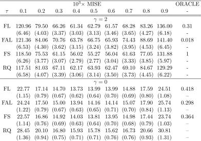
Table 2.1: The MISE and ORACLE proportions of different methods in Example 2.1.

103_{×MISE ORACLE}

τ 0.1 0.2 0.3 0.4 0.5 0.6 0.7 0.8 0.9

-γ = 2

FL 120.96 79.50 66.26 61.34 62.79 61.57 68.28 83.26 136.00 0.31 (6.46) (4.03) (3.37) (3.03) (3.13) (3.46) (3.65) (4.27) (6.18) -FAL 121.36 84.06 70.76 63.78 66.75 65.93 74.43 88.69 141.40 0.018

(6.53) (4.30) (3.62) (3.15) (3.24) (3.82) (3.95) (4.53) (6.45) -FS 118.50 75.53 61.15 56.02 55.27 56.04 61.63 77.05 131.88 1 (6.26) (3.77) (3.07) (2.79) (2.77) (3.04) (3.33) (3.85) (5.97) -RQ 117.51 81.03 67.11 62.17 63.93 62.47 69.10 84.67 129.29 -(6.58) (4.07) (3.39) (3.06) (3.14) (3.50) (3.73) (4.45) (6.22)

-γ = 0

FL 22.77 17.14 14.70 13.73 13.99 13.99 14.88 17.59 24.51 0.418 (1.15) (0.79) (0.67) (0.62) (0.64) (0.70) (0.69) (0.80) (1.08) – FAL 24.24 17.50 15.00 13.94 14.16 14.14 15.07 17.90 25.74 0.298

(1.22) (0.79) (0.67) (0.63) (0.65) (0.71) (0.70) (0.84) (1.13) – FS 22.57 16.86 14.92 14.03 13.81 13.95 14.98 17.44 23.74 0.364

(1.14) (0.76) (0.69) (0.63) (0.64) (0.70) (0.68) (0.79) (1.03) – RQ 28.45 20.10 16.80 15.93 15.78 15.62 16.73 20.66 30.81 – (1.36) (0.94) (0.75) (0.71) (0.71) (0.76) (0.76) (0.93) (1.31) –

The values in the parentheses are the standard errors of103×M ISE. MISE: Mean of Integrated

Squared Errors; ORACLE: the proportion of times where the model is selected correctly among 500 simulations. FL: Fused LASSO; FAL: Fused Adaptive LASSO; FS: Fused Sup-norm; FAS: Fused Adaptive Sup-norm; RQ: Regular Quantile Regression.

Table 2.1 contains the results for Example 2.1 with both γ = 2 and γ = 0. When γ = 2, the slope coefficientsβ(τ) vary across quantile levels. For this scenario, the group-wise shrinkage method FS performs the best with the smallest MISE and the highest

ORACLE. The FL method performs slightly better than FAL, possibly due to the

vari-ation in the adaptive weight estimate.

the conventional RQ method. Similar toγ = 2, FL is better than FAL in terms of MISE and ORACLE. This is largely due to the fact that the quantile slope coefficients are too

close to be distinguished when they are truly constant. In fact, the ideal component-wise

adaptive weights are supposed to be identical. The FL method, which does not assign any

weight, is equivalent to assigning equal component-wise weights. However, FAL adopts the

weights calculated from the RQ estimates with certain degree of variations, particularly in

the tails. Consequently, FAL has lower ability than FL for shrinkingd2 =β(0.2)−β(0.1) and d9 =β(0.9)−β(0.8) to zero (see Table 2.2).

Example 2.2. To further demonstrate the role of adaptive component-wise weights,

we consider a more complex univariate example. Let xi ∼ U(0,1) for i = 1, . . . ,500.

Assume Qτ(xi) =α(τ) +β(τ)xi for any 0< τ <1, where α(τ) =α+ Φ−1(τ) and

β(τ) =     

β−γΦ−1(0.49) +γΦ−1(τ) if 0< τ <0.49

β if 0.49≤τ <1,

with α = 0, β = 3, and γ = 15. To generate data, we first generate a quantile level ui ∼

U(0,1) and let yi =α(ui) +β(ui)xi. Therefore, for the quantiles τ = {0.1,0.2, . . . ,0.9},

β(τ) varies for τ = 0.1, . . . ,0.4, but remains as a constant for τ = 0.5, . . . ,0.9.

In this setting,β(τ) has different patterns across τ. Adaptive weights are expected to lead to more efficient shrinkage by controlling the shrinkage speeds of different coefficient

differences dk = β(τk)−β(τk−1), k = 2, . . . ,9. By assigning larger weights to the upper quantiles at whichβ(τ) is a constant, FAL achieves much higher ORACLE and TP at the upper five quantiles than FL (see Table 2.2). This suggests that if the interquantile slope

differences are well distinguished, employing adaptive weights can effectively improve the

Example 2.3. We generate data in the same way as in Example 2.2, but we let

β(τ) =           

β−γΦ−1(0.21) +γΦ−1(τ) if 0< τ <0.21

β if 0.21≤τ ≤0.59

β−γΦ−1(0.59) +γΦ−1(τ) if 0.59< τ <1,

with α = 0, β = 3, and γ = 15. We first generate a quantile level ui ∼ U(0,1) and let

yi =α(ui) +β(ui)xi, where xi ∼ U(0,1) for i = 1, . . . ,500. Therefore, for the quantiles

τ ={0.1,0.2, . . . ,0.9},β(τ) is a constant at quantile levels τ = 0.3,0.4,0.5, but varies in the other two quantile regions.

Results in Table 2.2 show that FAL has a clearly higher ORACLE than FL when

the interquantile slope differences are well distinguished. Moreover, when the trued’s are zero (d4 =d5 = 0), FAL is more likely to shrink them to zero by assigning larger adaptive weights. However, for d6 that is truly nonzero, FAL shrinks it to zero incorrectly more often than FL. This is possibly due to the large variation of the initial estimates around

the boundary quantile (τ = 0.6) where β(τ) changes from a constant to be varying inτ.

Example 2.4. In this example, we consider a bivariate case with p = 2. The data are generated from

yi =α+β1xi,1 +β2xi,2+ (1 +γxi,2)ei, i= 1, . . . ,200,

where xi,1

i.i.d

∼ U(0,1), xi,2

i.i.d

∼ U(0,1), ei i.i.d

∼ N(0,1), α = 1, β1 =β2 = 3. Therefore, the τth conditional quantile of Y given x1 and x2 is

Table 2.2: Percentage of correctly identifying dk =β(τk)−β(τk−1) over 500 simulations in Examples 2.1-2.3.

Example 2.1, γ= 2, TP

d26= 0 d36= 0 d46= 0 d56= 0 d6 6= 0 d7 6= 0 d8 6= 0 d9 6= 0 ORACLE

FL 0.69 0.89 0.93 0.91 0.94 0.92 0.89 0.67 0.31

FAL 0.65 0.66 0.67 0.65 0.65 0.67 0.67 0.62 0.02

Example 2.1, γ= 0, TP

d2= 0 d3= 0 d4= 0 d5= 0 d6 = 0 d7 = 0 d8 = 0 d9 = 0 ORACLE

FL 0.91 0.82 0.81 0.78 0.79 0.77 0.82 0.88 0.42

FAL 0.84 0.81 0.84 0.85 0.87 0.81 0.83 0.81 0.30

Example 2.2, TP

d26= 0 d36= 0 d46= 0 d56= 0 d6 = 0 d7 = 0 d8 = 0 d9 = 0 ORACLE

FL 1.00 1.00 1.00 0.99 0.50 0.66 0.67 0.81 0.25

FAL 0.96 0.97 0.97 0.84 0.78 0.98 0.98 0.96 0.52

Example 2.3, TP

d26= 0 d36= 0 d4= 0 d5= 0 d6 6= 0 d7 6= 0 d8 6= 0 d9 6= 0 ORACLE

FL 1.00 1.00 0.45 0.55 0.74 1.00 1.00 1.00 0.21

FAL 1.00 1.00 0.88 1.00 0.32 0.99 1.00 1.00 0.30

TP: percentage of correctly identifying each dk =β(τk)−β(τk−1), k= 2, . . . ,9 over 500

simula-tions. ORACLE: overall percentage of correctly shrinking all zerodk’s to zero and nonzero dk’s

as nonzero.

where α(τ) = α+ Φ−1(τ), β1(τ) = β1 and β2(τ) = β2 +γΦ−1(τ). Unlike β1(τ), which stays invariant for allτ,β2(τ) is constant whenγ = 0 but it varies across τ when γ 6= 0. As a group-wise shrinkage method, FAS either shrinks all interquantile slope

differ-ences dk,l = βk,l −βk−1,l, l = 1,2, k = 2, . . . ,9 to be exactly zero, or none of them to

be zero. Consequently, as shown in Table 2.3, when γ = 2, FAS has higher ORACLE than FL and FAL. By imposing two distinguished group-wise weights on two groups of

interquantile slope differences, FAS leads to better model selection results than FS. We

compare FL and FAL in Table 2.4. When the true d’s are indeed zero, FAL has higher TP

FAL may suffer from over-shrinkage problem in the varying regions.

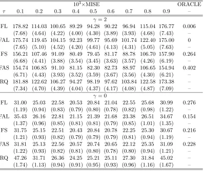
Table 2.3: The MISE and ORACLE proportion of different methods in Example 2.4 with γ = 2 andγ = 0, respectively.

103×MISE ORACLE

τ 0.1 0.2 0.3 0.4 0.5 0.6 0.7 0.8 0.9 –

γ = 2

FL 178.82 114.03 100.65 89.29 94.28 90.22 96.94 115.04 176.77 0.006 (7.68) (4.64) (4.22) (4.00) (4.30) (3.89) (3.93) (4.68) (7.43) – FAL 175.74 119.45 104.15 92.23 99.77 95.69 101.74 122.40 175.00 0 (7.65) (5.10) (4.52) (4.20) (4.61) (4.13) (4.31) (5.05) (7.63) – FS 156.21 107.46 91.09 80.49 79.45 81.17 88.78 106.70 157.90 0.264

(6.68) (4.41) (3.88) (3.54) (3.45) (3.63) (3.57) (4.26) (6.19) – FAS 154.74 106.85 91.10 81.15 82.30 82.73 88.97 106.65 154.94 0.402

(6.71) (4.43) (3.93) (3.52) (3.59) (3.67) (3.56) (4.30) (6.21) – RQ 181.88 122.62 106.27 94.27 98.19 97.62 103.84 122.58 173.38 – (7.34) (4.70) (4.39) (4.04) (4.37) (4.17) (4.08) (4.87) (7.09) –

γ = 0

FL 31.00 25.03 22.58 20.53 20.84 21.04 22.55 25.68 30.99 0.276 (1.19) (0.94) (0.83) (0.79) (0.80) (0.78) (0.82) (0.98) (1.22) – FAL 35.43 26.16 22.81 21.15 21.39 21.68 23.38 26.51 34.67 0.154

(1.37) (0.96) (0.85) (0.81) (0.81) (0.79) (0.85) (1.01) (1.35) – FS 31.75 25.15 22.51 20.43 20.84 20.78 22.25 25.30 30.67 0.216

(1.21) (0.93) (0.82) (0.79) (0.79) (0.79) (0.81) (0.94) (1.19) – FAS 31.81 25.13 22.56 20.57 20.74 20.65 22.12 25.35 31.09 0.228

(1.22) (0.93) (0.82) (0.81) (0.80) (0.78) (0.80) (0.94) (1.21) – RQ 47.26 31.71 26.36 24.25 25.21 25.11 27.30 31.84 45.02 – (1.74) (1.13) (0.94) (0.91) (0.95) (0.93) (0.96) (1.16) (1.67) –

Table 2.3 also shows the results whenγ = 0. As we expect, all the proposed shrinkage methods yield significantly smaller MISEs than RQ when the slope coefficients are

con-stant for each predictor. However, similar to Example 2.1, the quantile slope coefficients

adaptive weights from playing effective roles. Thus, FAL has less estimation efficiency

(higher MISE) and worse selection accuracy (lower ORACLE) than FL, especially in the

tails where the initial quantile estimates are more variable.

Table 2.4: True Proportion of True Positive (TP) for each interquantile difference dk,l

in Example 2.4 with γ = 2 and γ = 0, respectively. The interquantile slope differences dk,l = βk,l −βk−1,l, l = 1,2, k = 2, . . . ,9. For γ = 2, the true coefficients dk,1 = 0, but dk,2 6= 0 for allk. For γ = 0, dk,l = 0 for allk and l.

d2,1 d3,1 d4,1 d5,1 d6,1 d7,1 d8,1 d9,1 d2,2 d3,2 d4,2 d5,2 d6,2 d7,2 d8,2 d9,2

γ = 2

FL 0.79 0.69 0.62 0.58 0.59 0.62 0.79 0.61 0.85 0.92 0.92 0.92 0.92 0.89 0.87 0.58 FAL 0.79 0.80 0.81 0.77 0.82 0.79 0.80 0.79 0.63 0.67 0.67 0.66 0.69 0.65 0.69 0.58

γ = 0

FL 0.93 0.83 0.80 0.75 0.76 0.78 0.83 0.91 0.92 0.85 0.83 0.80 0.78 0.78 0.85 0.91 FAL 0.848 0.808 0.85 0.82 0.84 0.82 0.82 0.83 0.81 0.82 0.85 0.82 0.84 0.83 0.83 0.80

2.4.1

The Comparison of Different Group-wise Weights in FAS

h

max{|d˜k,l|:k= 2, . . . , K}

i−1 ,

where ˜dk,l is the initial estimator obtained from the conventional quantile regression. In

fact, for each l, ˜wk,l is the same for different k’s. Hence the notation can be simplified as

˜

wl. However, we can define the group-wise weight in many other ways, and the

asymp-totic properties will not be affected. In this subsection, we access the sensitivity of FAS

against the choice of different group-wise weights.

As we know, the group-wise weight ˜wl aims to distinguish groups with constantβ(τ)

from those with τ-dependent ones. In other words, ˜wl controls the group-wise shrinkage

quantile slope coefficients corresponding to the first predictor are constant, but vary

across quantiles for the second one. In this scenario, the ideal group-wise weight ˜w1should be much larger than ˜w2 so thatθ(1), the first group of interquantile slope differences, can be shrunk to zero much faster than θ(2). On the other hand, if both groups of quantile slope coefficients are constant, say γ = 0 in Example 2.4, the ideal group-wise weights should be close, so that θ(1) and θ(2) would be shrunk to zero at the same speed. Due to the characteristics of adaptive group-wise weights, we study some other ones in this

subsection. The asymptotic properties are not affected by different choices of ˜wl.

Choice 1 (weighted average of ˜d’s): we define the group-wise weight as the average of initial slope difference estimates, but weighted by their variances. Explicitly speaking,

define

˜ w_l(1) =

"( |d2˜,l|

var( ˜d2,l)

+. . .+ | ˜ dK,l|

var( ˜dK,l)

)

( 1 var( ˜d2,l)

+. . .+ 1 var( ˜dK,l)

)#−1

, l = 1, . . . , p.

Since the initial estimates of quantile slope coefficients have different variations at

differ-ent quantile levels, ˜w_l(1) aims to downweight ˜dk,l with a larger variation corresponding to

the lth _predictor.

Choice 2 (median of ˜d’s): another choice of adaptive group-wise weights can be defined as

˜

w(2)_l =hmedian{|d˜2,l|, . . . ,|d˜K,l|}

i−1

, l= 1, . . . , p.

Using median instead of mean can result in a more robust measurement of the group-wise

weights, especially for groups with non-constant quantile slope coefficients.

and define

˜

w(3)_l =hmedian{|d˜k,l|/sd( ˜dk,l), k= 2, . . . , K}

i−1

, l= 1, . . . , p,

where sd( ˜dk,l) is the standard deviation of ˜dk,l. In this choice, ˜w_l(3) aims to downweight

˜

dk,l with a larger standard deviation, and it is robust to the outliers of estimated ˜dk,l for

each l.

Table 2.5 shows the results of FAS with four different choices of the group-wise weight

in Example 2.4 with γ = 0 and γ = 2, respectively. Results suggest that FAS is quite insensitive to different group-wise weights. Therefore, we stay with ˜wl in the subsequent

Table 2.5: The MISE and ORACLE of FAS by adopting different group-wise weights in Example 2.4 with γ = 0 and γ = 2, respectively.

103×MISE ORACLE

τ 0.1 0.2 0.3 0.4 0.5 0.6 0.7 0.8 0.9

-γ = 0

regular 31.92 25.26 22.59 20.59 20.78 20.63 22.13 25.40 31.29 0.226 choice 1 32.09 25.34 22.73 20.59 20.78 20.85 22.23 25.45 30.94 0.234

(1.22) (0.94) (0.83) (0.79) (0.80) (0.79) (0.80) (0.96) (1.20) – choice 2 32.43 25.34 22.67 20.56 20.93 20.87 22.35 25.65 31.03 0.234

(1.22) (0.94) (0.83) (0.78) (0.80) (0.79) (0.81) (0.94) (1.19) – choice 3 32.21 25.25 22.64 20.50 20.92 20.94 22.43 25.68 31.08 0.23

(1.23) (0.93) (0.83) (0.78) (0.80) (0.79) (0.81) (0.95) (1.20) –

γ = 2

regular 154.74 106.85 91.10 81.15 82.30 82.73 88.97 106.65 154.94 0.402 choice 1 154.32 107.18 91.48 80.57 81.65 82.29 88.91 106.40 154.03 0.438

(6.75) (4.55) (3.91) (3.49) (3.56) (3.67) (3.57) (4.30) (6.18) – choice 2 154.30 107.71 91.79 81.03 81.61 81.82 88.58 106.04 153.58 0.464

(6.81) (4.57) (3.96) (3.50) (3.55) (3.63) (3.53) (4.31) (6.30) – choice 3 154.04 107.39 91.65 81.28 82.50 82.64 89.23 106.76 153.98 0.458

(6.79) (4.54) (3.92) (3.56) (3.60) (3.64) (3.59) (4.31) (6.29) –

Different choices of group-wise weights. Regular: 1/max, that is, the regular group-wise weight

discussed in Section 2.2.2; choice 1: average ofds, weighted by their variances; choice 2: median˜

of ds; choice 3: median of˜ ds, but weighted by their standard deviations. The values in the˜

2.5

Real Data Study

In this section, we apply the proposed methods to analyze the international economic

growth data, which were originally taken from Barro and Lee (1994)[2] and later studied

by Koenker and Machado (1999)[18]. This data set is available as ‘barro’ in R package

quantreg.

The data set contains 161 observations. The first 71 observations correspond to 71

countries and their averaged annual growth percentages of per Capita Gross Domestic

Product (GDP growth) from period 1965-1975 are recorded. The rest 90 observations are

for period 1975-1985. Some countries may appear in both periods. There are 13

covari-ates involved in total: the initial per capital GDP (igdp), male middle school education (mse), female middle school education (f se), female higher education (f he), male higher education (mhe), life expectancy (lexp), human capital (hcap), the ratio of eduction and GDP growth (edu), the ratio of investment and GDP growth (ivst), the ratio of public consumption and GDP growth (pcon), black market premium (blakp), political instabil-ity (pol) and growth rate terms trade (ttrad). All covariates are standardized to lie in the interval [0,1] before analysis, and we focus on τ ={0.1,0.2, . . . ,0.9}. Our purpose is to investigate the effects of covariates on multiple conditional quantiles of the GDP growth.

Koenker and Machado (1999)[18] studied the effects of covariates on certain

condi-tional quantiles of the GDP growth by using the convencondi-tional quantile regression method

(RQ). In this study, we consider simultaneous regression of multiple quantiles by

employ-ing the proposed adaptively weighted penalization methods FAL and FAS, and select the

penalization parameter by minimizing the AIC value as described in Section 2.3

(Re-sults are in Tables 2.6 and 2.7 for FAL and FAS, respectively). Figures 2.1-2.2 show

levels for 13 covariates. In each plot, the shaded area is the 90% pointwise confidence

band constructed from the inversion of rank score test described in Koenker and Bassett

(1982)[16]. The points connected by solid lines correspond to the estimated quantile

co-efficients from RQ, while the points connected by dashed lines are FAL estimates, and

the stars with dashed lines are FAS estimates. The FAS shrinks the slope coefficients

of mhe, ivst and blakp to be constant over τ, while FAL tends to shrink neighboring quantile coefficients to be equal, resulting in piecewise constant quantile coefficients. In

contrast, the solid lines (RQ) are more variable compared to the dashed lines (FAL and

FAS), since RQ can not make any shrinkage.

To further verify the shrinkage results, we conduct hypothesis tests to check the

constancy of slope coefficients by using the R function “anova.rqlist” inquantreg package. This function is based on the Wald test described in Koenker and Bassett (1982)[16] and

can be used to test if the slope coefficients are identical across different specified quantiles.

For the covariate ivst, for example, the anova test for equality of quantile coefficients at τ = 0.1, . . . ,0.9 results in a p-value of 0.9324, suggesting that the effect of ivst does not vary significantly across the nine quantile levels, which agrees with the results from

FAL and FAS, where the nine quantile coefficients are shrunk to be a constant. On

the other hand, for the covariate pol, the equality test on the quantile coefficients at τ = 0.1, . . . ,0.9 results in a p-value of 0.000996, implying that the effect of pol varies across the 9 quantile levels. More specifically, the equality test at τ = 0.5, . . . ,0.9 shows the significant differences in quantile slope coefficients. However, if we test the equality

of slope coefficients atτ = 0.1, . . . ,0.5, the null hypothesis was failed to be rejected. This agrees with the results from FAL, which shrinks the first 5 quantile coefficients to be a

constant, but keeps the upper quantile coefficients vary.

valida-tion. The data are randomly split into a testing set with 50 observations and a training

set with the rest 111 observations. For each method, we estimate the quantile coefficients

based on the training set, denoted as ˆβ(τj), j = 1, . . . ,9 and predict the τjth conditional

quantile of the GDP growth on the testing set. Prediction Error (PE), used to assess the

prediction accuracy, is defined as

PE = 9 X

k=1 50 X

j=1

ρτk{yj−x

T

jβˆ(τk)},

where {(yj,xj), j = 1, . . . ,50} are in the testing set. We repeat the cross validation 200

times and take the average of PE. For FAL, the mean PE is 253.33 (s.e.=1.68), while it

is 252.80 (s.e.=1.71) for FAL and 258.94 (s.e.=1.65) for RQ. The results show that both

proposed penalization approaches yield higher prediction accuracy than the conventional

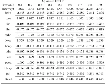
Table 2.6: Estimated quantile slope coefficients for economic growth data by FAL. The tuning parameter is selected by AIC. Neighboring estimates with underlines beneath are identical.

Quantile levelτ

Variable 0.1 0.2 0.3 0.4 0.5 0.6 0.7 0.8 0.9 Intercept 0.075 0.584 1.082 1.445 1.871 2.438 2.650 3.284 3.843

igdp -2.548 -2.548 -2.548 -2.580 -2.580 -2.580 -2.580 -2.844 -2.896

mse 1.012 1.012 1.012 1.012 1.111 1.463 1.463 1.463 1.463

fse -0.194 -0.194 -0.194 -0.246 -0.246 -0.246 -0.246 -0.367 -0.367

fhe -0.075 -0.075 -0.075 -0.075 -0.075 -0.075 -0.075 -0.075 -0.075

mhe 0.172 0.172 0.172 0.172 0.172 0.172 0.226 0.226 0.226

lexp 1.359 1.359 1.359 1.359 1.359 1.359 1.359 1.359 1.359

hcap -0.410 -0.414 -0.414 -0.414 -0.414 -0.733 -0.733 -0.733 -0.733

edu -0.305 -0.305 -0.153 -0.153 -0.153 -0.153 -0.153 0.058 0.058

ivst 0.629 0.629 0.629 0.629 0.629 0.629 0.629 0.629 0.629

pcon -1.090 -1.090 -0.804 -0.804 -0.599 -0.599 -0.599 -0.599 -0.599

blakp -0.859 -0.859 -0.891 -0.891 -0.891 -0.891 -0.891 -0.891 -0.891

pol -0.742 -0.742 -0.742 -0.742 -0.742 -0.569 -0.569 -0.231 0.046

Table 2.7: Estimated quantile slope coefficients for economic growth data by FAS. The tuning parameter is selected by BIC. Neighboring estimates with underlines beneath are identical.

Quantile levelτ

Variable 0.1 0.2 0.3 0.4 0.5 0.6 0.7 0.8 0.9 Intercept 0.034 0.592 1.093 1.505 2.003 2.396 2.779 3.230 3.833

igdp -2.606 -2.601 -2.606 -2.611 -2.616 -2.621 -2.625 -2.630 -2.635 mse 1.097 0.998 0.899 0.998 1.097 1.195 1.294 1.393 1.436

fse 0.072 0.105 0.026 -0.053 -0.131 -0.210 -0.288 -0.367 -0.446 fhe -0.138 -0.109 -0.081 -0.052 -0.023 -0.052 -0.081 -0.109 -0.138 mhe 0.161 0.161 0.161 0.161 0.161 0.161 0.161 0.161 0.161

lexp 1.298 1.330 1.362 1.330 1.353 1.385 1.386 1.354 1.322 hcap -0.487 -0.498 -0.508 -0.519 -0.530 -0.540 -0.551 -0.561 -0.572

edu -0.355 -0.304 -0.253 -0.202 -0.150 -0.099 -0.058 -0.007 -0.058 ivst 0.612 0.612 0.612 0.612 0.612 0.612 0.612 0.612 0.612

pcon -1.001 -0.917 -0.833 -0.749 -0.665 -0.641 -0.557 -0.473 -0.389 blakp -0.935 -0.935 -0.935 -0.935 -0.935 -0.935 -0.935 -0.935 -0.935

0.2 0.4 0.6 0.8 -3 .5 -3 .0 -2 .5 -2 .0 ig d p

0.2 0.4 0.6 0.8

-0 .5 0 .0 0 .5 1 .0 1 .5 2 .0 2 .5 ms e

0.2 0.4 0.6 0.8

-1 .5 -1 .0 -0 .5 0 .0 0 .5 1 .0 1 .5 fs e

0.2 0.4 0.6 0.8

-1 .0 -0 .5 0 .0 0 .5 fh e

0.2 0.4 0.6 0.8

-0 .5 0 .0 0 .5 1 .0 mhe

0.2 0.4 0.6 0.8

0. 5 1 .0 1. 5 2 .0 le x p

0.2 0.4 0.6 0.8

-1 .0 -0 .5 0 .0 0 .5 hc ap

0.2 0.4 0.6 0.8

-1 .0 -0 .5 0 .0 0 .5 ed u

0.2 0.4 0.6 0.8

0 .2 0 .4 0. 6 0 .8 1. 0 1 .2 iv s t    

0.2 0.4 0.6 0.8

-1 .5 -1 .0 -0 .5 pc o n

0.2 0.4 0.6 0.8

-1 .2 -1 .0 -0 .8 -0. 6 -0. 4 bl ak p

0.2 0.4 0.6 0.8

-1 .0 -0 .5 0 .0 po l

0.2 0.4 0.6 0.8

0. 2 0 .4 0. 6 0 .8 1 .0 tt ra d

2.6

Theoretical Proof

Lemma 2.1 (Convexity Lemma) Let {hn(u) : u ∈ U} be a sequence of random

convex functions defined on a convex, open subset U of Rd_{. Suppose h(u) is a}

real-valued function on U for which hn(u) → h(u) in probability for each u ∈ U. Then for

each compact subset Kof U, sup_u∈K|hn(u)−h(u)| →0 in probability. Proof The proof can be found in [24].

Proof of Proposition 2.1 Define

Ln(δ) = K X k=1 n X i=1

ρτk{yi−z

T

ik,A(θA,0+n−1/2δ)} −ρτk(yi−z

T

ik,AθA,0)

,

where δ ∈ RK+s is bounded. The minimizer to Ln(δ), denoted as ˆδ, is n1/2(ˆθA−θA,0). Following the identity in [11], we have

ρτ(r−s)−ρτ(r) = −s{τ −I(r <0)}+

Z s

0

{I(r ≤t)−I(r≤0)}dt.

Therefore, Ln(δ) = −n−1/2

PK

k=1 Pn

i=1z

T

ik,A{τk −I(yi −zTik,AθA,0 < 0)}δ + PK

k=1B (k)

n ,

where

B_n(k) =

n

X

i=1

Z n−1/2zT_ik,Aδ

0

n

I(yi−zTik,AθA,0 ≤t)−I(yi−zTik,AθA,0 ≤0) o