DSOUZA, KEITH CECIL. Methodology for Assessing the Impact of Distributed Generation on Electric Power Systems. (Under the direction of Dr. Mesut E. Baran).
This study investigates the impacts that DG ( Distributed Generation), namely PV, has on the bulk power system and proposes methods to quantify the costs and benefits related to DG.
First, an overview of DG is presented, after which various impacts of DG are discussed. Lastly these impacts are segregated as costs and benefits, and are monetized.
This report first looks at the impacts of DG on the distribution system, particularly, the impact of high penetration PV at the end of a sample distribution feeder or laterals. The impacts are studied on the IEEE123 bus system as a case study. OpenDSS® is used to simulate the impacts.
The penetration levels are varied to observe over-voltages, voltage flickers, branch overloads, and reverse power flows. Benefits such as reduction in losses and deferral of upgrades are noted.
Similarly, costs incurred due to additional regulation equipment, equipment upgrades, etc. are considered. A final $/MWh value of avoided cost at the distribution level is arrived at.
The second part of this report studies the impacts of DG on the generation system. The aim
of this study is to provide a comprehensive method to study and evaluate the impacts DG on generator dispatch, with a focus on ramping issues. A case study is performed with a prototype
system. A method is then proposed to split the avoided cost (of the generation system) based on impacts. A production cost model is used to perform this study, the model has been implemented in Matlab®.
This report finally presents a single value of avoided costs ($/MWh) for each year of analysis. Further work can be performed to study the impact of different kinds of storage in this
© Copyright 2019 by Keith Cecil DSouza
by
Keith Cecil DSouza
A thesis submitted to the Graduate Faculty of North Carolina State University
in partial fulfillment of the requirements for the degree of
Master of Science
Electrical Engineering
Raleigh, North Carolina 2019
APPROVED BY:
_______________________________ _______________________________ Dr. Mesut E. Baran Dr. David Lubkeman
Committee Chair
ii DEDICATION
To My Parents
And
iii BIOGRAPHY
Keith Cecil Dsouza was born in Ribandar, Goa, India. He received his B.Engg. in Electrical and Electronics Engineering from Goa College of Engineering, Goa University in 2012. He
worked at Marico ltd. from 2012 to 2013 as a maintenance engineer at Baddi, Himachal Pradesh, India, and from 2013 to 2014 as a supply chain analyst at Mumbai, Maharashtra, India . He returned to his home state to work at Goa State Infrastructure and Development Corporation,
Panaji, Goa, India from 2014 to 2016 as an assistant manager (elect.).
He was accepted to North Carolina State University’s Master’s program in Electrical and
Electronics Engineering in the fall of 2016. He joined the FREEDM Systems Center as a research assistant in the summer of 2017 under the guidance of Dr. Mesut E. Baran. He has worked on a
CAPER project for Duke Energy related to DER evaluation.
iv ACKNOWLEDGMENTS
I wish to express my sincere gratitude to all the people who made this work possible. To my advisor, Dr. Mesut E. Baran, whose constant guidance, encouragement, technical
insight, patience, and faith in my abilities were instrumental in completing this work.
To my committee members, Dr. David Lubkeman, and Dr Wenyuan Tang, for dedicating their time and offering valuable suggestions and timely help.
To my research fellows at the FREEDM System Center. It is a pleasure to be part of such a vibrant team.
To my friends, near and far, who have been a constant source of encouragement.
v TABLE OF CONTENTS
LIST OF TABLES ... vi
LIST OF FIGURES ... vii
Chapter 1: INTRODUCTION ... 1
1.1. Types of DG ... 1
1.2. Services that DG can provide ... 3
1.3. Impact of DG... 4
1.4. Current scenario ... 5
1.5. Scope of thesis ... 5
Chapter 2: IMPACT OF DG ON THE DISTRIBUTION SYSTEM ... 7
2.1. Impact of DG... 7
2.2. Benefits of DG ... 10
2.3. Mitigation strategies for DG impacts ... 10
2.4. A methodology to quantify the costs and benefits of DG ... 13
2.5. Case study ... 18
Chapter 3: IMPACT OF DG ON THE GENERATION SYSTEM ... 33
3.1. Impact of DG... 33
3.2. Benefits of DG ... 35
3.3. Mitigation strategies for DG impacts ... 39
3.4. A methodology to quantify the costs and benefits of DG ... 39
3.5. Case study ... 45
Chapter 4: CONCLUSION ... 56
vi LIST OF TABLES
Table 1.1 Services provided to the utility by DG ... 3
Table 2.1 Voltage and overload issues ... 21
Table 2.2 Voltage Flicker – baseline and final value(Volts) ... 24
Table 2.3 Voltage Regulator Operations ... 25
Table 2.4 System Operating point without PV ... 26
Table 2.5 System operating point with PV ... 26
Table 2.6 Overload before and after PV ... 27
Table 2.7 Equipment Overloads – new capacity with PV ... 28
Table 2.8 System Performance with distributed irradiance ... 29
Table 2.9 Final Results of Distribution Study ... 31
Table 3.1 Generator Parameters ... 45
Table 3.2 Results of Simulation – Total Production Cost ... 51
Table 3.3 Results of Simulation with Distributed Irradiance ... 51
Table 3.3 Timeline of Costs ... 53
vii LIST OF FIGURES
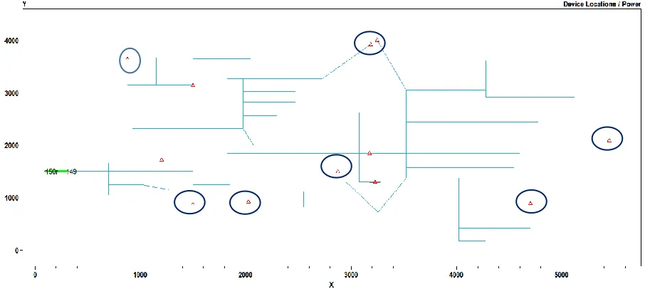
Figure 2.1 Prototype Distribution Feeder – Location of PV installation (circled) ... 18
Figure 2.2 Insolation Profile ... 19
Figure 2.3 Load profile ... 19
Figure 2.4 Voltage Violations across Feeder ... 22
Figure 2.5 Power density across Feeder ... 22
Figure 2.6 Insolation for PV trip and reset ... 23
Figure 3.1 Ramping and Bottoming Out ... 34
Figure 3.2 Displacement of Conventional Generation ... 36
Figure 3.3 Peak shifting ... 37
Figure 3.4 Displacement of Conventional Generation ... 43
Figure 3.5 Load, Total Generations – No PV ... 47
Figure 3.6 Generator Dispatch – No PV ... 48
Figure 3.7 Generator Ramping – No PV ... 48
Figure 3.8 Load, Total Generations – 40% PV ... 49
Figure 3.9 Generator Dispatch – 40% PV ... 49
Figure 3.10 Generator Ramping – 40% PV ... 40
Figure 3.11 Solar PV Output - 40% PV ... 40
1 CHAPTER 1. INTRODUCTION
The nature of electricity delivery, consumption, generation, and grids itself are changing, and changing rapidly due to Distributed Generation (DG). Instead of traditional, one-way delivery
of electricity from large, central station power plants located far from the load, via high voltage transmission lines, to lower voltage distribution lines, and, finally, to the home, technologies are now available directly to customers that allow them to generate their own electricity from their
rooftops.[1]
DG penetration has been rapidly increasing over the years, especially due to policy support
and the attractive value proposition it promises to consumers.[1]
Before we go into how DG is affecting the grid, we need to understand what is DG.
1.1. Types of DG
There are broadly six types of DG. Each type has their own unique operating characteristics and associated benefits and costs to the grid.
1 Solar PV: The fastest growing DG, solar PV systems use solar cells, formed into solar panels, to convert sunlight into electricity. Solar PV systems can be located on rooftops of
homes or commercial and industrial buildings or can be ground- mounted. The PV systems can be used to meet the energy requirements for the home or building or the energy from the system can be exported to the grid through the distribution system to be used by a
nearby load. [1]
2 the heat and uses it for many other purposes such as heating, cooling, domestic hot water,
and industrial processes. [1]
3 Wind: Distributed wind energy systems use wind energy to create power and are commonly installed on residential, agricultural, commercial, industrial, and—sometimes— community sites. The systems vary in size. A turbine for a home can be as large as a 10 kilowatt turbine, whereas a turbine for a manufacturing facility can be several megawatts.
Distributed wind systems can be connected on the customer’s side of the meter to meet its energy needs or directly to distribution to support grid operations or offset nearby loads.
[1]
4 Demand Response: DR can be used as a resource by utilities and grid operators to balance supply and demand. The use of DR as a resource can lower the cost of electricity in wholesale markets by avoiding the dispatch of more costly generation resources, which then could lead to lower retail rates. [1]
Although traditionally viewed as a peak reduction resource, DR can be used to increase consumption when there is excess generation, or more regularly to avoid
dispatching of more costly generation resources and enhance the efficiency of the grid. [1]
5 Energy Efficiency: EE is capable of providing both energy and demand savings. EE can be used by a utility to displace generation from other sources, such as coal, nuclear power,
natural gas, or any other supply-side resource. EE can provide a transmission and distribution benefit by allowing the utility to reduce or eliminate the need for upgrades or
3 1.2. Services that DG can provide
In order to understand the benefits and impacts DG provides, let us first understand the services that a grid provides/receives to/from customers.
Table 1.1. Services provided to the utility by DG[2].
Service Description
Op er ation al S er vice s
Energy Electricity produced (MWh)
Power /
Capacity
The amount of power (MW) available to the grid from a generating
resource at a point in time
Voltage Control
Regulation of the voltage required for transmission and distribution lines to transport and deliver power
Frequency regulation
Small short-term generation changes on the grid required to maintain a frequency of 60 hertz on transmission lines
Reliability/ Preventing blackouts in, and maintaining reliable electricity delivery to,
distribution circuits in event of a disturbance. Resilience
Black-start/outag
e recovery
Providing start up power to generating units after an outage
Pl an n in g S er vice s Primary Reserves
Generating units or demand resources that respond immediately to stabilize grid frequency in the event of a system disturbance or loss of generating
units
Secondary
Reserves
4 Table 1.1. Services provided to the utility by DG[2] (continued).
Plan n in g S er vice
s Tertiary Reserves
Generating units or demand resources that allow primary and secondary
reserves to return to their normal reserve state after the event of a system disturbance or loss of a generating unit
Flexibility
The ability to provide energy to the grid on a flexible basis which can be
useful for balancing variable demand, and variable supply from DG
M isc. S er vice s Capital Expenditure investment deferral
The ability to reduce or eliminate a shortfall in energy or capacity so that capital expenditures for upgrades at existing facilities or investment in new centralized resources are not necessary
Reduction of
losses
The reduction of transmission and distribution losses on the grid
Arbitrage of energy price
differentials
Buying power at times when power prices are lower or when there is excess generation supply and storing it for the purpose of selling it back
to the grid when demand and prices are higher
1.3. Impacts of DG
While DG has the potential to benefit the grid, it also comes with its share of problems. Increasing penetration of DG has created a host of impacts on the generation system such
as excess generation, out of order dispatch, frequent and faster ramping of units. [10]
Similarly, high penetration of DG on the distribution system can cause local overloads and
5 The impacts along with the benefits will be individually reviewed in the sections dealing
with the distribution and generation system respectively, in this report.
1.4. Current scenario
Given the overall impetus given to DG and its large scale adoption, many papers have endeavored to quantify the costs and benefits of DG on various sections of the bulk power system. However, most of these reports focus on the generation and transmission system. The focus on the
distribution system is limited to the avoided losses and capacity benefits. [4][5][6][7][8]. The integration costs need to be considered along with the benefits.
A bulk of the distributed generation is being connected to the distribution system and it’s expected to increase, hence it is necessary to study the impacts on the generation and distribution
system in tandem.
1.5. Scope of thesis
This thesis attempts to present a comprehensive and holistic approach to Assessing the
Impacts of Distributed Generation on Electric Power Systems.
In order to fully study the effects on the distribution system, a static power flow analysis is
not sufficient, the entire timeseries of load and PV needs to be analyzed, as issues could occur outside the peak load period of the system [3].
Hence, an analysis on the entire timeseries data is carried out, and the results are used to
allocate costs and benefits in this thesis. This analysis should ideally include the behavior of fast-acting inverters, dynamic loads, and automatic voltage control devices on the feeders. For the
6 The general approach adopted for both, the generation and distribution system, is the
avoided cost approach; the net benefits DG offers to the utility is the cost that it avoids.[1] This report concentrates on the impacts and benefits of Solar PV, however, the approach
presented can be applied to all types of DG.
This study considers only a single insolation patter for all the DG installations, however, some studies [13] [14] have shown that DG spread across a large area has a smoothing effect on
the overall insolation pattern. This in turn reduces the ramping and intermittency of variable resources (DG) to some extent. This effect on the generation and distribution system has been also
7 CHAPTER 2.IMPACT OF DG ON THE DISTRIBUTION SYSTEM
In this chapter we will look at the impacts on the distribution system, the distribution system comprises of the last mile connectivity to customer premises. The benefits and effects of
DG are most pronounced in this part of the electric power system.
Let us first look at the impacts and the benefits before we attempt to quantify them.
2.1. Impact of DG
The following impacts are seen on the distribution system.
1 Local Overloads: The loading on feeders needs to be studied as High Penetration DG systems tend to cause significant reverse power flow, especially in light load conditions (where the PV supplies most of the load). This reverse power flow can cause the loading
of a section of the distribution system to be larger than the corresponding loading during peak loading conditions without DG in the system, even to the point of overloading.[2][3]
2 Load Masking: High penetration DG systems tend to hide downstream loads (especially during peak generation) from the upstream source. Monitoring of loads occurs at the substation, making it difficult to estimate the real load. Thus, any circuit modification or
planning related activity to be carried out needs to factor in the native load calculations and should not be based solely on measurements collected from the feeder. [2][3]
3 Cold Load Pickup: In absence of power supply for a considerable amount of time (>30mins), loss of diversity occurs when the power supply is restored. This results in an inrush current several times the peak load. PV systems may be tripped during faults. If they
8 than the peak load current (with PV), which presents a critical planning issue for circuit
capacity. [2][3]
4 Over-voltages: Local pockets of high voltage might appear across the feeder especially during light loads due to excess power generation. This can impact the life of electrical equipment, degrading insulation, and cause PV systems to trip. [2][3]
5 Increased Substation Voltage: In absence of voltage regulators at the substation, or even with regulators with insufficient headroom, there is a possibility for the substation voltage to rise beyond permissible limits, causing protection circuits to trip. [2][3]
6 Voltage Flicker: Variations in PV resulting from variations in insolation levels can cause pulsations in the customer’s voltage. There might be noticeable variations in the
illumination levels at the customer’s premises. This variation is a lot slower than the ac
frequency of the power supply. The amount of permissible flicker is a great decider in the limit of the PV power that can be connected to the distribution system. [2][3]
7 Increased AVR switching: Varying insolation levels can cause a significant increase in the switching instances of the voltage regulating equipment i.e. capacitor banks, voltage
regulators, tap changer etc. This could cause premature failure of the equipment. [2][3]
8 Improper regulator functioning: If a PV system is connected immediately downstream of a voltage regulator with line drop compensation enabled, the regulator will not sense the
9 9 Reverse Power flow to adjacent circuits: Significant reverse power flows could exceed the interruption ratings of circuit protection elements, and could also result in sympathetic tripping of adjacent circuits due to fault feeding. [2][3]
10 Temporary over voltage: Load rejection and islanding can cause a temporary (few seconds to few minutes, depending on the time delay of the regulation equipment) increase in the voltage of the section. The PV system needs to act fast and trip in such a situation
in-order to prevent damage to the connected equipment. [2][3]
11 Transient over voltage: Very short duration (few milliseconds or less) voltage transients either caused by lightning or switching operations, this can cause surges in reactive elements in the grid [2][3]
12 Voltage regulator runaway: High penetration DG can cause significant reverse power flows through voltage regulators. In such a scenario, the voltage regulator may try to regulate the power flow on the source side (if the mode is enabled). The substation is a
strong source and will not respond. The regulator will keep changing its taps till it reaches its limits. This will result in higher or lower than permissible voltages on the PV side of the
regulator depending on which side the taps have changed. [2][3]
13 Effect of large installations: When DG is spread across a large geographic area, the individual DG installations peak at different points. Clouds cannot cover the entire
installation at once, thus DG spread across a large area will have a smoother output profile than if the entire system were to be concentrated in one area [13][14].
10 2.2. Benefits of DG
The following benefits can be associated with DG:
1 Energy: DG can supply the energy requirements of the individual households thus reducing the requirement from the distribution system. The local supply of energy also reduces losses in many cases as the energy no longer flows over large distances to supply the requirement. [2][3]
2 Capacity: DG can reduce the capacity requirement of various equipment in the distribution system due to peak reduction. This could be in the form of capacity deferral. [2][3]
3 Voltage support: DG can improve the voltage profile across a feeder/ provide voltage support similar to voltage regulators/capacitor banks but injecting power at ‘preferred’
locations. [2][3]
4 Microgrid operation: DG can provide resiliency to disturbances/outages in the grids by providing power to the islanded portion of the grid (if permitted by the regulators) in the
event of a blackout. [2][3]
2.3. Mitigation strategies for DG impacts
Before we can quantify the costs and benefits related to DG we need to understand the mitigation strategies that are required to be employed to offset the impacts of DG on the grid.
11 2 Load Masking: Load masking does not cause a tangible impact on the grid on its own, nevertheless, care must be taken to factor in the actual connected load while planning future upgrades or other planning activities. [2][3]
3 Cold Load Pickup: As with the case of load masking, the cold load pickup current due to loss of diversity must be computed without DG’s contribution to arrive at proper sizing of equipment. [2][3]
4 Over-voltages: Local over-voltages can be resolved by limiting the amount of DG that can be connected to the point in the distribution network. Relocation and/or addition of voltage
regulation equipment may also be needed to prevent the occurrence of local over-voltages. Inverters with reactive power control can also be employed to draw reactive power and
negate the voltage rise. [2][3]
5 Increased Substation Voltage: Again, the simple solution to prevent increased substation voltage would be to limit the amount of DG that can be connected downstream. Addition
of voltage regulation equipment and/or inverter with reactive power control can also be considered. [2][3]
6 Voltage Flicker: Several strategies can be considered in order to limit voltage flicker, such as the installation of express feeder lines to the substation for large DG facilities, relocation of smaller facilities or their point of interconnection wherever feasible, intelligent inverters
with volt-var control, installation of new voltage regulation equipment, as well as setting tighter tolerances and shorter delays to existing voltage regulation equipment. Storage
12 grid may also be considered. The final scheme that gets used would depend on the
permissible limit of voltage flicker as well as the economics of the solution. [2][3]
7 Increased AVR switching: The variability of DG cause a varying voltage profile which the regulator must constantly smoothen. Depending on the amount of permissible flicker, the voltage tolerance and the time delay of the regulators can be tweaked to reduce AVR operations. Advanced inverter control strategies can also be employed. Limiting the size of
DG as well as the relocation of the DG/ AVR may also be considered. Storage technologies can be used to store energy during peak insolation and inject this power during load peaks.
This will cause a flatter load profile and consequentially a flatter voltage profile. [2][3]
8 Improper regulator functioning: Relocation of the AVR/ DG to prevent load masking at the AVR with line drop compensation, will alleviate the problem. Remote metering of the unmasked load and communication to the AVR equipment can also be considered. [2][3]
9 Reverse Power flow to Adjacent circuits: A detailed study related to the fault levels needs to be conducted. Relay pickups and coordination may need to be altered to prevent tripping of protection devices. [2][3]
10 Temporary and transient over voltage: Inverters with low and high voltage ride through capabilities and a scheme with variable trip/clearing time can be employed to prevent the occurrence of temporary over/under voltage. Sacrificial arresters are another option,
however, these may be difficult to coordinate with utility arrestors. [2][3]
13 feed-forward direction. Adding additional regulation and or relocating voltage regulation
equipment are other ways to address this problem.[2][3]
2.4. A methodology to quantify the costs and benefits of DG
The proposed method to quantify the costs and benefits is as follows:
Step 1.Time horizon: Set a time horizon for the analysis (20 to 30 years). Divide the time horizon into smaller blocks (3 to 5 years). Choose an appropriate load growth and DG growth to apply as a factor to each block.
Step 2.Impact Study and Assessment: Conduct an impact study for each block of data. The impact analysis needs to focus on the critical points of the system. The critical points are during low load and low PV, low load and high PV, high load and low PV, high load and
high PV. A base case is also setup for comparison purposes.
The results of the analysis are pooled together and compared with the base case to assess the following impacts:
a. Voltage Violation: Any node where a load is connected whose voltage is less than 0.95pu or greater than 1.05pu is considered to have voltage issues. Mitigation
strategies discussed above will need to be implemented in order to address these issues, from the time period in which the violations begin.
14 computed for the given equipment. The maximum capacity (kW) of this magnitude
over the planning period needs to be considered for mitigation purposes.
c. Voltage Flicker: If the voltage between successive instances of time(1sec) rises or falls by more than 4v (on a 120v base), the node is experiencing voltage flicker issues. Voltage flicker is generally checked at the point of interconnection between the grid and the PV setup. A further analysis is conducted by simulating a PV
system outage and reconnection, and then measuring the voltage dip/rise at the point of interconnection, and the change in voltage is studied. If the change in voltage is
more than the aforementioned bounds, mitigation strategies are adopted.
d. Regulator operations: The operations of each regulator are obtained from the impact study. These are compared to the base case. The magnitude of the increase in regulator operations is computed. Any increase in operations has a detrimental effect on the lifespan of the regulator. This decrease in the lifespan is calculated and
a replacement schedule is calculated based on this information.
e. Avoided Losses: The system losses in the base year are considered to be the benchmark. The system losses in the subsequent years with load growth and PV growth considered are compared with this benchmark value. Any reduction in losses (from the benchmark year) can be attributed to the increase in PV penetration.
This net reduction will result in monitory savings to the utility
15 utilization in excess of 95% can be computed as the additional capacity required in
the distribution system.
g. Effect of large installations: In order to simulate the effects of large installations, a time displacement is introduced in the insolation of each DG installation. This displacement can be varied to study the effects of different geographies. DG spread across a small area will have a smaller shift in their incident solar radiation, larger
areas will have a bigger displacement.
Step 3.Mitigation: Specific mitigation strategies have been discussed in the previous section. In this section we will discuss how to apply them.
a. Overloading: The maximum extent of overloading computed in the assessment is used to ascertain the sizing (kW) of the equipment or line section to be replaced. The first instance of that equipment overloading is the point at which the replacement would occur.
b. Voltage violations/flicker: As discussed above, the general practice for mitigating voltage violation/flicker issues would be to tweak the existing AVR settings and/or
install new AVR equipment immediately downstream of the PV installation. The settings are adjusted such that the voltage doesn’t go beyond 0.95pu to 1.05pu, also the band center is set such that the voltage doesn’t drop/rise too much after a
contingency at the PV plant.
Any adjustment to the settings of existing regulators in order to reduce the
16 cost of having solar PV in the circuit. Hence, instead of considering a mitigation
strategy to reduce the regulator operations, we consider the cost associated with increased regulator operations in the next section.
Step 4.Economic Analysis:
Based on the mitigation strategies employed in (Step 3), we compute the total cost of mitigation.
a. Overloading: The total capacity (kW) required based on the mitigation study to reduce the overloading is summed up. The unit cost of circuit upgrades is
considered to be 55$ per kW[9], the total cost of mitigation is computed by multiplying this unit rate with the total circuit upgrades.
b. Voltage regulator installation: The cost of the AVR equipment including installation costs are considered at the point in time that voltage violations/flicker issues creep up. Operating and maintenance costs are considered on a yearly basis
from the next year onwards.
c. Voltage regulator operations: Consider the regulators in the base case to have the standard life of a regulator. The increase in operations will reduce this life by a proportional percentage. Given, the new scenario, the additional number of regulators required can be computed from : original life/reduced life - 1. The cost
17 d. Avoided Losses: The amount of reduction in losses computed for each block is converted to a dollar value using the prevalent cost of energy (12c/kWh). If the losses increase for some reason the value will be negative.
e. Avoided Capacity: Any additional capacity as computed in the assessment stage is converted to a dollar value using the cost of distribution system upgrades(55$/kW/year).
The costs and benefits calculated so far occur at various points of time, either on a recurring basis or as a onetime event. The net cost at each year is calculated by summing
the costs and benefits of the year. Since the value of money changes with time, we need to bring all the cost and benefits to a single reference year by means of the present worth
function. The discount rate/interest rate prevalent at the time (6%) may be considered for the analysis. An inflation rate/escalation rate of 2% is considered as well. The present value of the amount at their respective years are then summed up to give a single dollar amount.
18 2.5. Case study
Using the proposed methodology, a case study was performed on a prototype distribution feeder system with 123 nodes.
Figure 2.1. Prototype Distribution Feeder – Location of PV installations (circled)
According to the methodology:
Step 1.Time horizon: A time horizon of 20 years was considered for this exercise. The 20-year period was divided into five 5 year blocks, wherein the load grew at 2% every block from
the base value. The initial PV penetration was 0% for the first block, 10% for the next block, 20% for the next, and 40% for the last block. As shown in Figure 2.1 above, eight
PV sites were selected at the end of various branches in the feeder, each of equal capacity. The PV rating of each system varies from 0kW for no penetration, and 47.8kW, 97.5kW, and 198.75kW for subsequent blocks.
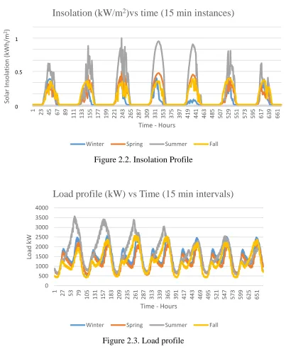
19 Figure 2.2. Insolation Profile
Figure 2.3. Load profile
Step 2.Impact Study and Assessment: An impact study was conducted for each block of data with OpenDSS. The system was tested at critical points of its operation across a year. The points consisted of a weeklong load profile of these critical points along with their
respective insolation data. The data, as presented above, consisted of the following critical points: low load with low insolation (fall), low load with high insolation (spring), high load
1 23 45 67 89
111 133 155 177 199 221 243 265 287 309 331 353 375 397 419 441 463 485 507 529 551 573 595 617 639 661
Sola r In so lat ion (k Wh /m 2)
Time - Hours
Insolation (kW/m
2)vs time (15 min instances)
Winter Spring Summer Fall
1 0.5 0 0 500 1000 1500 2000 2500 3000 3500 4000
1 27 53 79
105 131 157 183 209 235 261 287 313 339 365 391 417 443 469 495 521 547 573 599 625 651
Lo
ad
k
W
Time - Hours
Load profile (kW) vs Time (15 min intervals)
20 with high insolation (summer), and high load with low insolation (winter). These points
would capture the worst-case impacts on the distribution system with varying DG penetration.
Reports that contained the system operating points, voltage levels, equipment loading levels, and regulator operations were extracted from the simulations for each of the critical points of each block.
The results of the simulation are as follows:
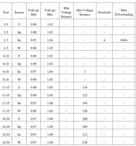
a. Voltage Violations and Overloads: From the voltage reports generated in the simulation, the minimum and maximum circuit voltages for each critical point were computed. Also, the number of instances where the voltage in the circuit dropped
below 0.95 pu, or increased beyond 1.05 pu i.e. voltage violations were computed. The results are presented in Table 2.1. It is observed that voltage violations start occurring after the PV penetration level exceeds 20% in the 15 - 20 year block.
The current overload reports generate the loading of all conductors/ equipment exceeding 100 percent of their nominal rating. The criterion however is
21 Table 2.1. Voltage and overload issues
Year Season Volts pu
Min Volts pu Max Min Voltage Instance Max Voltage
Instance Overloads
Max %Overloading
1-5 F 0.98 1.02 - - - -
1-5 Sp 0.98 1.02 - - - -
1-5 Su 0.97 1.04 - - 4 104%
1-5 W 0.98 1.02 - - - -
6-10 F 0.98 1.03 - - - -
6-10 Sp 0.98 1.03 - - - -
6-10 Su 0.97 1.04 - 2 - -
6-10 W 0.98 1.03 - - - -
11-15 F 0.98 1.05 - 134 - -
11-15 Sp 0.98 1.05 - 125 - -
11-15 Su 0.97 1.06 - 194 - -
11-15 W 0.98 1.05 - 136 - -
16-20 F 0.97 1.08 - 288 - -
16-20 Sp 0.97 1.08 - 289 - -
16-20 Su 0.97 1.08 - 312 - -
16-20 W 0.97 1.08 - 238 - -
In general, the violations were seen to be occurring at the end of the branches, especially in the area where the PV was installed. Some mitigation will
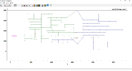
22 Figure 2.4. Voltage Violations across Feeder – Green: Overvoltage, Blue: Normal Voltage
Figure 2.5. Power density across Feeder
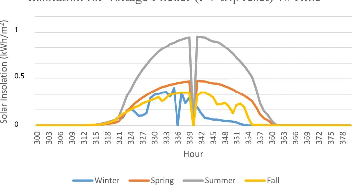
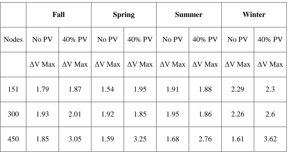
23 connected to the grid. The maximum rise and fall are computed for each node and
compared across seasons and penetration. The voltage flicker limit considered is around 4 volts on a 120 volt base.
The PV was cut off and restarted during peak insolation to simulate the worst-case flicker that would manifest at the points of interconnection. This was simulated by modifying the insolation data as shown below. For the purpose of
flicker simulation, the time series load data had a resolution of 1 second. Figure 2.6 illustrates this. The results of this simulation are presented in Table 2.2.
Figure 2.6. Insolation for PV trip and reset
300 303 306 309 312 315 318 321 324 327 330 333 336 339 342 345 348 351 354 357 360 363 366 369 372 375 378
Solar In
solat
ion
(kWh
/m
2)
Hour
Insolation for Voltage Flicker (PV trip reset) vs Time
Winter Spring Summer Fall
1
0.5
24 Table 2.2. Voltage Flicker – baseline and final value (Volts)
Fall Spring Summer Winter
Nodes No PV 40% PV No PV 40% PV No PV 40% PV No PV 40% PV
ΔV Max ΔV Max ΔV Max ΔV Max ΔV Max ΔV Max ΔV Max ΔV Max
151 1.79 1.87 1.54 1.95 1.91 1.88 2.29 2.3
300 1.93 2.01 1.92 1.85 1.95 1.86 2.26 2.6
450 1.85 3.05 1.59 3.25 1.68 2.76 1.61 3.62
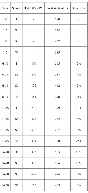
c. Voltage Regulator operation: The voltage regulator operations were computed by comparing the tap position at the previous operating point with the new tap position
at each data point in the simulation. Any change was counted as an operation. The sum of operations for each regulator during each season was computed both with
and without PV.
It is seen that as the PV penetration increase, so does the number of regulator operations. This would translate to an additional cost in the form of faster
25 Table 2.3. Voltage Regulator Operations
Year Season Total With PV Total Without PV % Increase
1-5 F - 290 -
1-5 Sp - 254 -
1-5 Su - 457 -
1-5 W - 383 -
6-10 F 300 295 2%
6-10 Sp 240 257 -7%
6-10 Su 472 462 2%
6-10 W 381 390 -2%
11-15 F 296 299 -1%
11-15 Sp 277 262 6%
11-15 Su 496 467 6%
11-15 W 391 398 -2%
16-20 F 335 305 10%
16-20 Sp 305 266 15%
16-20 Su 499 474 5%
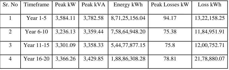
26 d. Avoided Losses and Avoided Capacity
The difference between the system operating point (Losses) with and without PV in the system will give us the extent of avoided losses, this value can
be monetized with the cost of energy. The operating point with and without PV is shown in Table 2.4 and Table 2.5 respectively. The avoided losses may be negative if the losses increase with the PV penetration.
Table 2.4. System Operating point without PV
Sr. No Timeframe Peak kW Peak kVA Energy kWh Peak Losses kW Loss kWh
1 Year 1-5 3,584.11 3,782.58 8,71,25,156.04 94.17 13,22,158.25
2 Year 6-10 3,655.79 3,795.09 8,88,67,659.16 97.00 13,61,823.00
3 Year 11-15 3,727.47 3,792.11 9,06,10,162.28 98.41 13,81,655.37
4 Year 16-20 3,799.16 3,870.92 9,23,52,665.40 100.39 14,09,420.69
Table 2.5. System Operating point with PV
Sr. No Timeframe Peak kW Peak kVA Energy kWh Peak Losses kW Loss kWh
1 Year 1-5 3,584.11 3,782.58 8,71,25,156.04 94.17 13,22,158.25
2 Year 6-10 3,236.13 3,359.44 7,58,64,948.20 75.38 11,84,951.91
3 Year 11-15 3,301.09 3,358.33 5,44,77,877.15 75.8 12,00,752.71
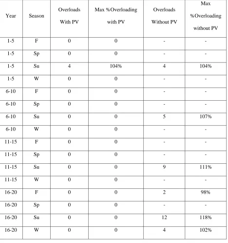
27 Table 2.6. Overloads before and after PV.
Year Season
Overloads
With PV
Max %Overloading
with PV
Overloads
Without PV
Max
%Overloading
without PV
1-5 F 0 0 - -
1-5 Sp 0 0 - -
1-5 Su 4 104% 4 104%
1-5 W 0 0 - -
6-10 F 0 0 - -
6-10 Sp 0 0 - -
6-10 Su 0 0 5 107%
6-10 W 0 0 - -
11-15 F 0 0 - -
11-15 Sp 0 0 - -
11-15 Su 0 0 9 111%
11-15 W 0 0 - -
16-20 F 0 0 2 98%
16-20 Sp 0 0 - -
16-20 Su 0 0 12 118%
28 Table 2.7. Equipment Overloads – new rating with PV
"Element" % Loading New Capacity kW
"Line.L117" 111.12% 5,409.19
"Line.L58" 105.09% 5,321.43
"Line.L55" 110.12% 4,760.71
"Line.L116" 105.76% 4,572.22
"Line.L52" 113.38% 4,901.64
Total 24,965.18
Table 2.6 presents the list of overloads and the time at which they occur. Table 2.7 presents a list of all the equipment that needs to be replaced and the
maximum capacity that is required.
e. Effect of large installation: The system considered for this study is scaled to different geographies by introducing different time shifts to emulate the effect of geographic displacement.
The following time shifts are considered:
29 The Table 2.8 below shows the aggregated results for the different
insolation patters for each of the above cases. The insolation displacement was considered to start from the left side of the sample feeder.
Table 2.8. System Performance with shifted irradiance.
Sr. No % PV Time Shift Peak kW Peak kVA Energy kWh Peak Losses kW Loss kWh
1 40% 0min 3,366.26 3,429.85 1,88,86,308.28 78.81 21,78,880.07
2 40% ±15min 3,293.86 3,429.92 1,88,77,442.73 78.42 21,66,014.64
3 40% ±30mins 3,215.12 3,322.83 1,88,71,203.30 73.19 21,49,429.23
When the results for the 40% penetration case (shifted vs unshifted
insolation) are compared, it is seen that there is a steady decrease in the peak kW and kWh of the load as well as the losses in the feeder.
Step 3.Mitigation: The mitigation strategies were based on the type of violations observed in the feeder.
a. Overloading: No additional overloading has been observed when PV is added to the feeder.
b. Voltage violations and regulator operations: The method adopted for mitigating the voltage violations and voltage flicker was to install voltage regulating devices at the point of interconnection between each PV and the grid. The AVRs would regulate the voltage downstream from the PV.
30 third 5-year period of our simulation; hence we consider this as the point at which
the voltage regulator investment took place. The cost of a regulator is taken to be $10,000 (each).
Step 4.Economic Analysis: Based on the results of the impact assessment, we now monetize the impacts and benefits as follows:
a. Overloading: The extent of excess capacity required is multiplied by the cost of mitigation 55$ per kW. The is the cost of mitigating the overloads [6].
b. Voltage regulators installation: The cost of the SVR equipment including installation costs are considered at the point in time that voltage violations/flicker issues crept up. Operating and maintenance costs are considered on a yearly basis
from the next year onwards.
c. Voltage regulator operations: The cost of a regulator multiplied by the number of additional regulators will give the total cost of this mitigation. However, since the
number of regulator operations have returned to baseline values, this cost was not considered
d. Avoided Losses: The amount of reduction in losses computed for each block is converted to a dollar value using the prevalent cost of energy (12c/kWh). If the losses increase for some reason the value will be negative.
31 simply summing them up. The aforementioned interest and inflation rates were used. The
results are as follows:
Table 2.9. Final Results of Distribution Study
%
PV Yr
Avoided Energy Avoided Losses Avoided Losses Additional Regulator Cost + O&M Differed Cost Net Benefits with PV $/MWh
MWh kWh $ $ $ $
0 1 0 0 0 0 0
0 2 0 0 0 0 0
0 3 0 0 0 0 0
0 4 0 0 0 0 0
0 5 0 0 0 0 0
10 6 13,002.71 176,871.09 21,224.53 1,373,084.69 982,932.98 75.59
10 7 13,002.71 176,871.09 21,224.53 14,115.53 1.09
10 8 13,002.71 176,871.09 21,224.53 13,316.53 1.02
10 9 13,002.71 176,871.09 21,224.53 12,562.77 0.97
10 10 13,002.71 176,871.09 21,224.53 11,851.67 0.91
20 11 36,132.29 180,902.66 21,708.32 -80,000.00 -30,707.33 -0.85
20 12 36,132.29 180,902.66 21,708.32 -200 10,688.98 0.30
20 13 36,132.29 180,902.66 21,708.32 -200 10,083.94 0.28
20 14 36,132.29 180,902.66 21,708.32 -200 9,513.15 0.26
20 15 36,132.29 180,902.66 21,708.32 -200 8,974.67 0.25
40 16 73,466.36 -769,459.38 -92,335.13 -200 -36,426.11 -0.50
40 17 73,466.36 -769,459.38 -92,335.13 -200 -34,364.25 -0.47
40 18 73,466.36 -769,459.38 -92,335.13 -200 -32,419.11 -0.44
40 19 73,466.36 -769,459.38 -92,335.13 -200 -30,584.06 -0.42
40 20 73,466.36 -769,459.38 -92,335.13 -200 -28,852.89 -0.39
Total Cost $ 880,686.46
Total Avoided Energy MWh 613,006.77
32 interesting to note that at low penetrations (10%), the utility will benefit the most out of the
PV systems in the grid. As the penetration goes up, various mitigation techniques are needed in order to maintain the power quality. The costs of mitigation start adding up
33 CHAPTER 3. IMPACT OF DG ON THE GENERATION SYSTEM
In this chapter we will look at the impacts on the generation system, it comprises of the generating resources e.g. base load generation, intermediate generation and peaker plants. The Due
to the change in net load caused by DG, the cost of will change. DG tends to lower the cost of generation at lower penetrations, however, as often seen, DG tends to increase the cost of generation at higher penetrations owing to the need for expensive peaker units. [1][2]
Let us first look at the impacts and the benefits before we attempt to quantify them.
3.1. Impact of DG
The impacts of DG are as follows:
1 Energy Cost Reduction: DG exerts downward pressure on the energy prices. The revenue lost by the utility – assuming a volumetric rate regime – will be two-fold; reduced revenues from lower energy sales, as well as from a lower unit rate of energy. [1][10][11]
2 Ramp Rates: Baseload plants like coal and nuclear are limited by how fast they can pick up or drop the load on them. Variability of DG can require excessive ramping from generating resources, possibly exceeding their limits. Any sustained excess/shortfall of
34 Figure 3.1 Ramping and Bottoming Out – [10]
3 Bottoming Out: At high penetrations of DG, the conventional generating resources will have to be ramped down. There is a limit up to which they can be ramped down without shutting them down. If the supply exceeds that point, the utilities will have no option other
than turning off these resources as they have bottomed out. Since DG is not a constant source of energy, these generating resources will need to be turned on again, resulting in
additional costs to the utility. [10]
4 Power Balance: At any point in the electric grid, the total supply must balance the total demand. The non-dispatchable nature of privately owned DG systems increases the
complexity of balancing supply with demand. As mentioned earlier, any sustained shortfall/excess of power in the grid will create instabilities. There is a limit up to which
35 5 Effect of large installations: DG installations spread over a large geographic area have a smoothing effect on the overall power output of the DG resources that is seen by the generation system. This results in reduced ramping and lower intermittency. [13][14]
3.2. Benefits of DG
The benefits on the generation system are as follows:
1. Energy: High penetration PV will displace the resource on the margin; normally gas turbines. Thus, the presence of PV in the system reduces the need for energy generated from the resource at the margin. This is called avoided energy. Peaking resources cost more
than baseload plants and hence this substitution is beneficial to the utility. However, as the penetration goes up the resources being displaced also changes. The time of the solar peak
and its correlation with the system peak is also important in understanding which resource is displaced. Figure 3.2 illustrates this issue.
Also, lower energy requirements can help utilities operate their generating
36 Figure 3.2 Displacement of Conventional Generation – [2]
2. Capacity: High penetration PV can displace/defer the need for new capacity resources. The demand that is offset can also be used as reserve capacity. In addition to the reduction in demand due to PV there could be a reduction in demand due to peak loss reduction.
Lower capacity demand at the generation level can be used to switch off costly gas turbine peaker plants due to the flatter load profile. With a sufficient increase in DG
37 Figure 3.3. Peak shifting – Georgia Power[10]
3. Risk: DG (PV) produces roughly constant-cost power compared to fossil fuel generation, which is tied to potentially volatile fuel prices. DG can provide a “hedge” against price
volatility, reducing risk exposure to utilities and customers. Utilities engage in long term contracts for fuel prices. The cost of volatility is already built into this quantity. DG will reduce the requirement for fuel and hence, reduces the amount of volatility that the utility
is exposed to. This reduction can be considered as the avoided risk cost. [1]
38 a. The potential to reduce outages by reducing congestion along the T&D network.
As, power outages and rolling blackouts are more likely when demand is high, and the T&D system is stressed, PVs can reduce the peak demand, and hence, mitigate
this issue.
b. The ability to reduce large-scale outages by increasing the diversity of the electricity system’s generation portfolio with smaller generators that are geographically
dispersed.
c. Provide back-up power sources that are available during outages through the
combination of PV, control technologies, inverters, and storage.
5. Grid Support services: In addition to the benefits of energy and capacity, DG can provide additional grid support services like reactive supply and voltage control, frequency regulation, and operating reserves with the aid of advanced inverter technology. [1][2]
6. Environmental: DG (PV and wind) are considered to be clean sources of energy. They do not release CO2, SOx, and NOx as by-products during the course of energy production.
Other resources like land and water also are required in less quantity compared to
conventional energy resources. The costs incurred by utilities to mitigate the pollutants as well the cost that the utility has incurred to procure land and water would now be reduced or completely avoided as a result of energy production from DG. These costs can be termed
as avoided environmental costs. Care has to be taken while quantifying the values of CO2,
SOx, and NOx , as only costs that have been truly avoided can be transferred to customers
39 7. Social: The assumed social value from PV is based on any job and economic growth benefits that PV brings to the economy, including jobs and higher tax revenue. The value of economic development depends on number of jobs created or displaced, as measured by
a job multiplier, as well as the value of each job, as measured by the average salary and/or tax revenue.[1][2]
3.3. Mitigation strategies for DG impacts
Having seen both the impacts and benefits of DG, let us now look at the mitigation strategies that can be employed to alleviate these impacts
1 Ramp Rates: Fast ramping gas turbines are added to generation fleets in order to meet the high ramp requirements of variable, unpredictable, and uncontrollable DG. Another alternative is to add storage devices to the grid. These store power during down ramps and
discharge power during up ramps. If these methods are not cost effective, then the DG may be curtailed as a last resort.[1][2]
2 Bottoming Out: Energy storage devices may be employed to store the excess power during off peak times and discharge it during peak demand periods. However, owing to the cost of storage, one may be more inclined to curtail DG than to deploy storage in the
system.[1][2]
3.4. A methodology to quantify the costs and benefits
40 Step 1.Time horizon: Set a time horizon for the analysis (20 to 30 years). Divide the time horizon into smaller blocks (3 to 5 years). Choose an appropriate load growth and DG growth to apply as a factor to each block.
Step 2.Impact Study and Assessment: An impact study needs to be performed for each block with the respective load and PV growth considered. The main challenge is to select suitable generator data for the impact study.
The cost function of the generators will be in the form:
𝐶 = 𝑚𝑖𝑛𝑃𝑔𝑖{∑(𝐴𝑖 + 𝐵𝑖 ∗ 𝑃𝑔𝑖+ 𝐶𝑖 ∗ 𝑃𝑔𝑖2)
𝑛
𝑖=1
∗ 𝑓𝑐𝑖+ 𝑉𝑂𝑀∗ 𝑃𝐺𝐼}
where, Ci is the production cost. A, B, C, and D are the coefficients for the
quadratic cost function. Fc is the fuel cost. Vom is the variable operating and maintenance
cost.
The ramp rate limits need to be factored into the simulation as a constraint. Since
we are working at the bulk system level, the aggregated load data is representative of the daily load curve. Congestion related impacts may not be considered.
The impact analysis is performed for four representative weeks: Fall, Spring, Summer, and Winter. The four different cases will have a different amount of generation
to be dispatched. The data resolution considered should reflect the intermittent variability of PV. Sunny day and cloudy day profiles for each of the four cases must be considered.
a. We now approach an optimization problem, wherein we need to minimize the cost
41 b. Objective function: Minimize the total production cost of all generators:
𝐶 = 𝑚𝑖𝑛𝑃𝑔𝑖{∑(𝐴𝑖 + 𝐵𝑖∗ 𝑃𝑔𝑖 + 𝐶𝑖∗ 𝑃𝑔𝑖2)
𝑛
𝑖=1
∗ 𝑓𝑐𝑖}
c. Power Limits: The generator’s output should be within its power output limits;
additional cases can be run for bottoming out where 𝑃𝑔𝑖_𝑚𝑖𝑛 = 0.
𝑃𝑔𝑖_𝑚𝑖𝑛 ≤ 𝑃𝑔𝑖 ≤ 𝑃𝑔𝑖_𝑚𝑎𝑥
d. Power Balance: If loss is neglected, the total generation should equal the total demand.
∑ 𝑃𝑔𝑖 = 𝑃𝑙𝑜𝑎𝑑+ 𝑃𝑙𝑜𝑠𝑠
𝑛
𝑖=1
e. Ramp Limits: The rate of change of the power output from different generators should be within the ramp rate limits of the generators.
|𝑃𝑛− 𝑃𝑛−1|
∆𝑡 ≤ 𝑅𝑎𝑚𝑝 𝐿𝑖𝑚𝑖𝑡 (
𝑀𝑊
𝑚𝑖𝑛)
f. Uptime and Downtime Constraints: The unit scheduling should be within the permissible limits of each generator
𝑈𝑛𝑖𝑡 𝑈𝑝𝑡𝑖𝑚𝑒 ≥ 𝑀𝑖𝑛. 𝑈𝑛𝑖𝑡 𝑈𝑝𝑡𝑖𝑚𝑒
𝑈𝑛𝑖𝑡 𝐷𝑜𝑤𝑛𝑡𝑖𝑚𝑒 ≥ 𝑀𝑖𝑛. 𝑈𝑛𝑖𝑡 𝐷𝑜𝑤𝑛𝑡𝑖𝑚𝑒
42 a. Avoided Energy: The difference between the cost of production with and without PV in the system for each block can be construed as a proxy for avoided energy costs.
b. Bottoming Out/Start-up Costs: If 𝑃𝑔𝑖 < 𝑃𝑔𝑖_𝑚𝑖𝑛 the generator needs to be shut down. If this generator needs to be turned on again, there will be a cost associated with this action. This cost is called the bottoming out cost/Startup Cost. The
difference between the startup costs with and without PV is the avoided startup costs. It might not always be feasible to turn down generators especially base load
plants.
∑ ∑ 𝑈𝑖𝑗 × 𝑆𝐶𝑖
𝑛𝑔𝑒𝑛
𝑖=1 𝑇𝑖𝑚𝑒
𝑗=1
Where Uij is the unit status vector (0 or 1) and SCi is the start-up cost of the
ith unit.
c. Avoided Fuel Costs: Solar PV will displace the marginal unit. The fuel that would have otherwise been used to produce energy is avoided as a result of this displacement by PV. The cost associated as a consequence is called Avoided Fuel
Cost.
∑ ∑ 𝒎𝒊𝒏(𝑴𝑷𝒊𝒋𝑼𝒊𝒋, 𝑫𝑺𝒐𝒍𝒊𝒋) × 𝑺𝑪𝒊
𝒏𝒈𝒆𝒏
𝒊=𝟏 𝑻𝒊𝒎𝒆
𝒋=𝟏
Where MPij is the power for the ith marginal unit at time = j, and DSolij is
43 Figure 3.4. Displacement of Conventional Generation[1]
Pictorially, if we consider a simple scenario with only three generators in the above figure, we see that PV has displaced all the peaking and some of the
intermediate resources. Thus the area under the curve between the peaking and the intermediate resources that has been displaced by PV multiplied by the production cost of that unit will yield the avoided fuel cost for that unit.
d. Avoided Capacity: In absence of the PV systems in the grid, the utility would have to upgrade its infrastructure in order to meet the growing demand. The peak
capacity of the generating resources is compared with the peak demand on the circuit, with and without PV for the entire planning period. If there is a shortfall in the case without PV, an upgrade is required. However, if this upgrade is differed by
a couple of years with PV in the circuit, then the difference in the present values of the two can be considered as an avoided capacity benefit.
44 with a net load shape that results from an artificially time shifted PV. These results
are then compared with the results of the case without the time shifting.
Step 3.Mitigation: Specific mitigation strategies have been discussed in the previous section. In this section we will discuss how to apply them.
a. Ramp Rate: The simulation is re-run after adding a peaker unit, in case of non-convergence. The production cost of the additional resource is factored into the
simulation. The present value of the capital cost (differed or otherwise), will yield the total avoided capacity cost, which can be positive or negative.
b. Bottoming Out: If the power output of the PV is more than minimum load generation level sustainable by the plants then the PV is curtailed. Storage may also
be employed but is not considered in the scope of this study.
Step 4.Economic Analysis: The process is similar to that adopted in the distribution system. The discount rate/interest rate prevalent at the time (6%) is considered for the analysis. An
inflation rate/escalation rate of 2% is considered as well. The present value of the amount at their respective years are then summed up to give a single dollar amount. This amount
45 3.5. Case Study
Step 1.Time horizon: A time horizon of 20 years was considered for this exercise. The 20-year period was divided into five 5 year blocks, wherein the load grew at 2% every block from
the base value. The initial PV penetration was 0% for the first block, 10% for the next block, 20% for the next, 40% for the last block.
The specification of the generators considered is as follows:
Table 3.1. Generator Parameter
P1 P2 P3 P4 P5 P6
Pmax MW 400 500 200 500 600 N*600
Pmin MW 50 150 50 150 0 0
A $ 373.5 403.61 253.24 388.93 194.28 194.28
B $/MW 7.62 7.519 7.836 7.573 7.77 7.77
C $/(MW)2 0.002 0.0014 0.0013 0.0013 0.0019 0.0019
SC $ 9.92 22.83 27.82 9.92 27.82 27.82
Ramp MW/min 5.5 3.056 9.9 4.5 8.9 8.9
The load shape considered for the distribution system is scaled to be comparable to the
46 Step 2.Impact Study and Assessment:
A production cost model is adopted to study the impacts of DG. The simulation is performed in two stages: Unit Commitment followed by Economic Dispatch.
a. Unit Commitment
i. The representative load data consists of 15-minute intervals. Since unit
commitment is performed on the load forecast and not the actual load data, noise is added to the actual data.
ii. The maximum load for each hour is calculated from the 4 intervals. This is
assumed to be the load for that hour.
iii. Gaussian noise is added to this value (±5%)
iv. For the PV data, the average of the actual data for each hour from the 4 – 15-minute interval is calculated. This is assumed to be the PV generation for that hour
v. The net load is calculated as the difference between forecasted load and the PV generation.
vi. A reserve margin of 8% is considered
47 b. Economic Dispatch
a. The net load is calculated from the actual load and actual PV.
b. The uptime and downtime constraints are not considered as the unit status
is already fixed.
c. The ramp limits are maintained
The above process is repeated for the 4 aforementioned cases, each time with a different penetration level.
The results of the simulation (for 7 days) of the base system without PV are shown
in Figure 3.5, 3.6 and 3.7.
48 Figure 3.6. Generator Dispatch – No PV
49 The results of the simulation (for 7 days) of the base system with 40% PV are shown
in Figure 3.8, 3.9, and 3.10. The PV profiles used is shown in Figure 3.11. The valley created by the solar PV is highlighted for the first day.
Figure 3.8. Load, Total Generations – 40% PV
50 Figure 3.10. Generator Ramping – 40% PV
Figure 3.11. Solar PV Output - 40% PV
51 We now look at quantifying the impacts of solar PV on the generation system. Table
3.2 shows the total production costs for each case. We see that it declines as the penetration increases however, it decreases at decreasing rate. This trend hints at a point of saturation
or even reversal, wherein there will be an increase in the production cost as the PV Penetration increases.
Table 3.2. Results of Simulation – Total Production Cost
Sr. No. % PV Total Production Cost ($) Total Startup Cost ($)
1 No 20,784,216.67 319.62
2 10 20,313,385.07 296.79
3 20 19,846,851.32 273.96
4 40 19,615,083.11 251.13
We now explore the effect of DG spread across a large geographic area. Table 3.3
shows the results of the simulation for 40% PV for the following cases:
1. ±15min shift
2. ±30min shift
Table 3.3. Results of Simulation with Distributed Irradiance
% PV Time Shift Total Production Cost ($) Total Startup Cost ($)
40 0 mins 19,615,083.11 251.13
40 ±15 mins 22,841,399.93 273.58
52 An interesting observation is the production costs and startup costs increase in this
scenario. However, it must be noted that no additional peakers were required to be added to the system.
Step 3.Mitigation
a. Ramp Rate: If the results from unit commitment and economic dispatch point towards insufficient ramping capability in the generation pool, a peaker plant is
added to the generation mix (process repeated till simulation runs). The cost of the peaker plant is considered to be $ 150,000.00/unit.
b. Bottoming Out: The PV is curtailed so that it does not turn negative. No Cost is associated with this action.
53 Table 3.4. Timeline of Costs
Sr. No. %PV Year Season Units Added
(Nos) Cost ($)
Avoided Production Cost($)
1 0 1-5 Fall - -
2 0 1-5 Spring - -
3 0 1-5 Summer - -
4 0 1-5 Winter - -
5 10 6-10 Fall - -
2,354,158.00
6 10 6-10 Spring - -
7 10 6-10 Summer - -
8 10 6-10 Winter - -
9 20 11-15 Fall - -
4,686,826.75
10 20 11-15 Spring - -
11 20 11-15 Summer - -
12 20 11-15 Winter - -
13 40 16-20 Fall - -
5,845,667.80
14 40 16-20 Spring 1 150,000.00
15 40 16-20 Summer 1 150,000.00
54 Step 4.Economic Analysis: Finally, we derive the levelized cost of energy ($/MWh) from all
the simulation scenarios studied. The results are presented in Table 3.5
Table 3.5. Final Results of Generation Study
%PV Year Mitigation Cost ($) Energy (MWh) Avoided
Avoided Production Cost
(Million $)
Present Value
(Million $) $/MWh
0 1 0 - - 0.000 -
0 2 0 - - 0.000 -
0 3 0 - - 0.000 -
0 4 0 - - 0.000 -
0 5 0 - - 0.000 -
10 6 0 65,013.55 2.354 1.869 28.75
10 7 0 65,013.55 2.354 1.798 27.66
10 8 0 65,013.55 2.354 1.731 26.62
10 9 0 65,013.55 2.354 1.665 25.61
10 10 0 65,013.55 2.354 1.602 24.65
20 11 0 180,661.43 4.687 3.070 16.99
20 12 0 180,661.43 4.687 2.954 16.35
20 13 0 180,661.43 4.687 2.843 15.73
20 14 0 180,661.43 4.687 2.735 15.14
20 15 0 180,661.43 4.687 2.632 14.57
40 16 300,000.00 367,331.79 5.846 2.997 8.16
40 17 0 367,331.79 5.846 3.040 8.28
40 18 0 367,331.79 5.846 2.925 7.96
40 19 0 367,331.79 5.846 2.815 7.66
40 20 0 367,331.79 5.846 2.708 7.37
Total Avoided Cost (Million $) 37.38
55 Figure 3.12. Variation of Total Avoided Energy Costs($/MWh) vs Time (Years)
In Figure 3.12 we see a generally increase trend for the total avoided costs, which
seems to be increasing at a decreasing rate. Year 16 includes the cost of the additional peaker units, hence the benefit is lower.
Summing up the present worth at each year we get a total benefit of $ 37.38 million
and a total avoided energy of 1,793,729.85 MWh tothe utility over the 20-year period. The benefit per unit energy is better at lower penetration. As the penetration goes up, peaker
plants (and/or storage) would need to be added to maintain a feasible generation. The costs of mitigation start adding up considerably at 20% penetration.
5.00 10.00 15.00 20.00 25.00 30.00 35.00
1 2 3 4 5 6 7 8 9 10 11 12 13 14 15 16 17 18 19 20
($
/MW
h
)
Years
![Table 1.1. Services provided to the utility by DG[2] (continued).](https://thumb-us.123doks.com/thumbv2/123dok_us/1571853.1193292/13.612.71.538.88.520/table-services-provided-utility-dg-continued.webp)