Likelihood-Free Inference in High-Dimensional Models

| INVESTIGATION

Likelihood-Free Inference in

High-Dimensional Models

Athanasios Kousathanas,*,†_{Christoph Leuenberger,}‡_{Jonas Helfer,}§_{Mathieu Quinodoz,**}

Matthieu Foll,††_{and Daniel Wegmann*},†,1 *Department of Biology and Biochemistry and‡Department of Mathematics, University of Fribourg, 1700 Fribourg, Switzerland,

†_{Swiss Institute of Bioinformatics, 1700 Fribourg, Switzerland,}§_{Electrical Engineering and Computer Science, Massachusetts} Institute of Technology, Cambridge Massachusetts 02139, **Department of Computational Biology, University of Lausanne, 1200 Lausanne, Switzerland, and††International Agency for Research on Cancer, 69372 Lyon, France

ABSTRACTMethods that bypass analytical evaluations of the likelihood function have become an indispensable tool for statistical inference in many fields of science. These so-called likelihood-free methods rely on accepting and rejecting simulations based on summary statistics, which limits them to low-dimensional models for which the value of the likelihood is large enough to result in manageable acceptance rates. To get around these issues, we introduce a novel, likelihood-free Markov chain Monte Carlo (MCMC) method combining two key innovations: updating only one parameter per iteration and accepting or rejecting this update based on subsets of statistics approximately sufficient for this parameter. This increases acceptance rates dramatically, rendering this approach suitable even for models of very high dimensionality. We further derive that for linear models, a one-dimensional combination of statistics per parameter is sufficient and can be found empirically with simulations. Finally, we demonstrate that our method readily scales to models of very high dimensionality, using toy models as well as by jointly inferring the effective population size, the distribution of

fitness effects (DFE) of segregating mutations, and selection coefficients for each locus from data of a recent experiment on the evolution of drug resistance in influenza.

KEYWORDSapproximate Bayesian computation; distribution offitness effects; hierarchical models; high dimensions; Markov chain Monte Carlo

T

HE past decade has seen a rise in the application of Bayesian inference algorithms that bypass likelihood cal-culations with simulations. Indeed, these generally termed likelihood-free or approximate Bayesian computation (ABC) (Beaumontet al.2002) methods have been applied in a wide range of scientific disciplines, including cosmology (Schafer and Freeman 2012), ecology (Jabot and Chave 2009, pro-tein-network evolution (Ratmannet al.2007), phylogenetics (Fan and Kubatko 2011), and population genetics (Cornuet et al. 2008). Arguably ABC has had its greatest success in population genetics because inferences in this field are fre-quently conducted under complex models for which likelihood calculations are intractable, thus necessitating inference through simulations.

Let us consider a modelMthat depends onnparameters u;creates dataD, and has the posterior distribution

pðujDÞ ¼R ℙðDjuÞpðuÞ ℙðDjuÞpðuÞdu;

wherepðuÞis the prior andℙðDjuÞis the likelihood function. ABC methods bypass the evaluation ofℙðDjuÞby perform-ing simulations with parameter values sampled from pðuÞ that generate D, which in turn is summarized by a set of m-dimensional statisticss:The posterior distribution is then evaluated by accepting such simulations that reproduce the statistics calculated from the observed data (sobs)

pðujsÞ ¼R ℙðs¼sobsjuÞpðuÞ ℙðs¼sobsjuÞpðuÞdu:

However, for models withm1 the conditions¼sobsmight be too restrictive and require a prohibitively large simulation effort. Therefore, an approximation step can be employed by relaxing the condition s¼sobs to ks2sobsk#d; where

Copyright © 2016 by the Genetics Society of America doi: 10.1534/genetics.116.187567

Manuscript received January 26, 2016; accepted for publication April 4, 2016; published Early Online April 6, 2016.

Supplemental material is available online atwww.genetics.org/lookup/suppl/doi:10. 1534/genetics.116.187567/-/DC1.

1_{Corresponding author: Department of Biology, University of Fribourg, Chemin du}

kx2ykis a distance metric of choice betweenxandyanddis a chosen distance (tolerance) below which simulations are accepted. The posteriorpðujsÞis thus approximated by

pðujsÞ ¼R ℙðks2sobsk#djuÞpðuÞ ℙðks2sobsk#djuÞpðuÞdu:

An important advance in ABC inference was the development of methods coupling ABC with Markov chain Monte Carlo (MCMC) (Marjoram et al.2003). These methods allow effi-cient sampling of the parameter space in regions of high likeli-hood, thus requiring fewer simulations to obtain posterior estimates (Wegmann et al.2009). The original ABC-MCMC algorithm proposed by Marjoramet al.(2003) is as follows:

1. If now atupropose to move tou9according to the transi-tion kernelqðu9juÞ:

2. SimulateDusing modelMwithu9and calculate summary statisticssforD.

3. Ifks2sobsk#d;go to step 4; otherwise go to step 1. 4. Calculate the Metropolis–Hastings ratio

h¼h

u;u9¼min 1;p

u9quu9 pðuÞqu9

! :

5. Accept u9with probabilityh; otherwise stay atu:Go to step 1.

The sampling success of ABC algorithms is given by the likelihood values, which are often very low even for relatively large tolerance values d: In such situations, the condition

ks2sobsk#d will impose a quite rough approximation to the posterior. As a result, the utility of the ABC approaches described above is limited to models of relatively low dimen-sionality, typically up to 10 parameters (Blum 2010; Fearnhead and Prangle 2012). The same limitation applies to the more recently developed sequential Monte Carlo sampling methods (Sissonet al.2007; Beaumontet al.2009). Despite these limitations ABC has been useful in addressing popula-tion genetics problems of low to moderate dimensionality such as the inference of demographic histories (e.g., Wegmann and Excoffier 2010; Brownet al.2011; Adrionet al.2014) or selection coefficients of a single locus (e.g., Jensenet al.2008). However, as more genomic data become available, there is increasing interest in applying ABC to models of higher dimensionality, such as to estimate genome-wide and locus-specific effects jointly.

To our knowledge, to date, three approaches have been suggested to tackle high dimensionality with ABC. Thefirst approach proposes an expectation propagation approxima-tion to factorize the data space (Barthelmé and Chopin 2014), which is an efficient solution for situations with high-dimensional data, but does not directly address the issue of high-dimensional parameter spaces. The second approach consists offirst inferring marginal posterior distributions on low-dimensional subsets of the parameter space [either one (Nott et al.2012) or two dimensions (Liet al.2015)] and

then reconstructing the joint posterior distribution from those. This approach benefits from the lower dimensionality of the statistics space when considering subsets of the param-eters individually and hence renders the acceptance criterion meaningful. The third approach achieves the same benefit by formulating the problem using hierarchical models, pro-posing to estimate the hyperparametersfirst, and thenfixing them when inferring parameters of lower hierarchies individ-ually (Bazinet al.2010).

Among these, the approach by Bazinet al.(2010) is the most relevant for population genetics problems, since those are frequently specified in a hierarchical fashion by modeling genome-wide effects as hyperparameters and locus-specific effects at lower hierarchies. In this way, Bazinet al.(2010) estimated locus-specific selection coefficients and deme-specific migration rates of an island model from microsatellite data. Furthermore, this approach has inspired the develop-ment of similar methods for estimating more complex migra-tion patterns (Aeschbacher et al.2013) and locus-specific selection from time-series data (Follet al.2015). However, this approach and its derivatives will not recover the true joint distribution if parameters are correlated, which is a common feature of such complex models.

Here, we introduce a new ABC algorithm that exploits the reduction of dimensionality of the summary statistics when focusing on subsets of parameters, but couples the parameter updates in an MCMC framework. As we prove below, this coupling ensures that our algorithm converges to the true joint posterior distribution even for models of very high dimen-sions. We then demonstrate its usefulness by inferring the effective population size jointly with locus-specific selection coefficients and the hierarchical parameters of the distribution offitness effects (DFE) from allele frequency time-series data.

Theory

Let us define the random variableTi¼TiðsÞas anmi-dimensional function ofs:We callTisufficientfor the parameteruiif the conditional distribution ofsgivenTidoes not depend onui: More precisely, letti;obs ¼TiðsobsÞ:Then

ℙs¼sobsjTi¼ti;obs;u

¼ℙ

s¼sobs;Ti¼ti;obsju

ℙTi¼ti;obsju

¼ ℙðs¼sobsjuÞ ℙTi¼ti;obsju

¼:giðsobs;u2iÞ; (1)

whereu2i¼ ðu1;. . .;ui21;uiþ1;. . .;unÞisuwith theith com-ponent omitted.

It is not hard tofind examples for parameter-wise sufficient statistics. Most common distributions are members of the exponential family, and for these, the density ofshas the form

fðsjuÞ ¼hðsÞexp

"

XK

k¼1

hkðuÞTkðsÞ2AðuÞ

For a given parameterui;the vectorTiðsÞconsisting of only thoseTkðsÞfor which the respective natural parameter func-tionhkðuÞdepends onuiis a sufficient statistic foruiin the sense of our definition. Some concrete examples of this type are studied below.

If sufficient statisticsTican be found for each parameterui and their dimension mi is substantially smaller than the dimension m of s;then the ABC-MCMC algorithm can be greatly improved with the following algorithm that we de-note ABC with parameter-specific statistics (ABC-PaSS) henceforth.

The algorithm starts at timet¼1 and at some initial pa-rameter valueuð1Þ:

1. Choose an index i¼1;. . .;naccording to a probability distributionðp1;. . .;pnÞwith

X

pi¼1 and allpi.0: 2. Atu¼uðtÞ proposeu9according to the transition kernel

qiðu9juÞwhereu9differs fromuonly in theith component:

u9¼ ðu1;. . .;ui21;ui9;uiþ1;. . .;unÞ:

3. SimulateDusing modelMwithu9and calculate summary statisticssforD. Calculateti¼TiðsÞandti;obs¼TiðsobsÞ: 4. Letdibe the tolerance for parameterui:Ifti2ti;obs_i#di;

go to step 5; otherwise go to step 1. 5. Calculate the Metropolis–Hastings ratio

h¼h

u;u9¼min 1;p

u9qiuu9 pðuÞqiu9ju

! :

6. Acceptu9with probabilityh; otherwise stay atu: 7. Increase tby one, save a new parameter valueuðtÞ¼u;

and continue at step 1.

Convergence of the MCMC chain is guaranteed by the following:

Theorem 1. For i¼1::n;if di¼0andTi is sufficient for parameter ui;then the stationary distribution of the Markov chain ispðujs¼sobsÞ:

TheProof for Theorem 1is provided in theAppendix. It is important to note that the same algorithm can also be applied to groups of parameters, which may be particularly relevant in the case of very high correlations between parameters that may render their individual MCMC up-dates inefficient. Also, the efficiency of ABC-PaSS can be improved with all previously proposed extensions for ABC-MCMC. To increase acceptance rates and render ABC-PaSS applicable to models with continuous sampling distribu-tions, for instance, the assumptiondi¼0 must be relaxed todi.0 in practice. This is commonly done in ABC appli-cations and will lead to an approximation of the posterior distributionpðujs¼sobsÞ:Because of the continuity of the summary statisticssand the sufficient statisticsTi;we the-oretically recover the true posterior distribution in the limit di/0: We can also perform an initial calibration ABC step tofind an optimal starting positionuð1Þand

tol-erancediand to adjust the proposal kernel for each param-eter (Wegmannet al.2009).

Materials and Methods

Implementation

We implemented the proposed ABC-PaSS framework into a new version of the software package ABCtoolbox (Wegmann et al. 2010), which will be made available at the authors’ website and will be described elsewhere.

Toy model 1: Normal distribution

We performed simulations to assess the performance of ABC-MCMC and ABC-PaSS in estimatingu1¼mandu2¼s2_{for a} univariate normal distribution. We used the sample meanx and sample varianceS2_{of samples of sizenas statistics.} Re-call that for noninformative priors the posterior distribution formisN ðx;S2_{=nÞand the posterior distribution for}

s2isx2 distributed withn21 d.f. Asmands2are independent, we get the posterior density

pm;s2¼fx;S2_=nðmÞ n21

S2 fx2;n21

n21 S2 s

2

:

In our simulations the sample size wasn¼10 and the true parameters were given bym¼0 ands2¼5:We performed 50 MCMC chains per simulation and chose effectively non-informative priors for mU½210;10and s2U½0:1;15: Our simulations were performed for a wide range of toler-ances (from 0.01 to 41) and proposal ranges (from 0.05 to 1.5). We did this exhaustive search to identify the combina-tion of these tuning parameters that allows ABC-MCMC and ABC-PaSS to perform best in estimatingmands2_{:We then} recorded the minimum total variation distance (L1) between the true and estimated posteriors over these sets of tolerances and ranges and compared it between MCMC and ABC-PaSS.

Toy model 2: General linear model

As a second toy model to compare the performance of ABC-MCMC and ABC-PaSS, we considered general linear models (GLMs) withmstatisticssbeing a linear function ofn¼m parametersu;

s¼Cuþe; eN ð0;IÞ;

whereCis a square design matrix and the vector of errorseis multivariate normal. Under noninformative priors for the pa-rametersu;their posterior distribution is multivariate normal

ujs NC9C

₂1 C9s;

C9C

₂1

:

B¼ 0 B B @

1=n 2=n 3=n . . . n=n n=n 1=n 2=n . . . n21=n

⋮ ⋮ ⋮ ⋱ 2=n

2=n 3=n 4=n . . . 1=n

1 C C A :

The normalization factor in the definition ofCwas chosen such that the determinant of the posterior variance is con-stant and thus the widths of the marginal posteriors are com-parable independently of the dimensionalityn. We used all statistics for ABC-MCMC and calculated a single linear com-bination of statistics per parameter for ABC-PaSS according to Theorem 2, using ordinary least squares. For the estima-tion, we assumed that u¼0 and the priors are uniform U½2100;100for all parameters, which are effectively non-informative. We started the MCMC chains at a normal de-viateNðu;0:01IÞ;i.e., around the true values ofu:To ensure fair comparisons between methods, we performed simula-tions of 50 chains for a variety of tolerances (from 0.01 to 256) and proposal ranges (from 0.1 to 8) to choose the com-bination of these tuning parameters at which each method performed best. We ran all our MCMC chains for 105 itera-tions per model parameter to account for model complexity.

Estimating selection and demography

Model: Consider a vector j of observed allele trajectories (sample allele frequencies) overl¼1;. . .;Lloci, as is com-monly obtained in studies of experimental evolution. We as-sume these trajectories to be the result of both random drift and selection, parameterized by the effective population size Ne and locus-specific selection coefficients sl; respec-tively, under the classic Wright–Fisher model with allelic fitnesses 1 and 1þsl:We further assume the locus-specific selection coefficients sl follow a DFE parameterized as a generalized Pareto distribution (GPD) with mean m¼0; shapex, and scales. Our goal is thus to estimate the joint posterior distribution

pðNe;s1;. . .;sL;x;sjjÞ

}YL

l¼1

ℙðjljNe;slÞpðsljx;sÞ

pðNeÞpðxÞpðsÞ:

To apply our ABC-PaSS framework to this problem, we ap-proximate the likelihood term ℙðjljNe;slÞ numerically with simulations, while updating the hyperparameters x and s analytically.

Summary statistics:To summarize the dataj;we used sta-tistics originally proposed by Follet al.(2015). Specifically, wefirst calculated for each locus individually a measure of the difference in allele frequency between consecutive time points as

Fs9¼1 t

Fs 1212~n22~n

ð1þFs=4Þ½121=ðnyÞ;

where

Fs¼ ðx2yÞ 2

zð12zÞ;

xandyare the minor allele frequencies separated byt gen-erations,z¼ ðxþyÞ=2;and ~nis the harmonic mean of the sample sizesnxandny:We then summed theFs9values of all pairs of consecutive time points with increasing and decreas-ing allele frequencies into Fs9i and Fs9d; respectively (Foll et al.2015). Finally, we followed Aeschbacheret al.(2012) and calculated boosted variants of the two statistics to take more complex relationships between parameters and statis-tics into account. The full set of statisstatis-tics used per locus was Fl=fFs9il;Fs9dl;Fs9i2l;Fs9d

2

l;Fs9il3Fs9dlg

We next calculated parameter-specific linear combinations forNeand locus-specificslfollowing the procedure developed above. To do so, we simulated allele trajectories of a single locus for different values ofNeandssampled from their prior. We then calculatedFlfor each simulation and performed a Box–Cox transformation to linearize the relationships between statistics and parameters (Box and Cox 1964; Wegmannet al. 2009). We thenfitted a linear model as outlined in Equation A3 to estimate the coefficients of an approximately suffi-cient linear combination ofFfor each parameterNeands. This resulted intsðFlÞ ¼bsFlandtNeðFlÞ ¼bNeFl:To com-bine information across loci when updating Ne; we then calculated

tNeðFÞ ¼

XL

l¼1 bNeFl;

where F¼ fF1;. . .;FLg In summary, we used the ABC approximation

ℙðjjjNe;sjÞ ℙtsðFlÞ2ts

Flobs,dsl;

ktNeðFÞ2tNeðFobsÞk,dNejNe;sjÞ:

Simulations and application

with an allele frequency $ 2% at $ 2 time points. There were 86 and 42 such loci for the control and drug-treated experiments, respectively. Further, we restricted our analysis of the data of the drug-treated experiment to the last nine time points during which drug was administered.

We performed all our Wright–Fisher simulations with in-house C++ code implemented as a module of ABCtoolbox. We simulated 13 generations between time points and a sample of size 1000 per time point. We set the prior forNe uniform on the log10 scale such that log10ðNeÞ U½1:5;4:5 and for the parameters of the GPD xU½20:2;1and for log10ðsÞ U½22:5;20:5: For the simulations where no DFE was assumed, we set the prior ofsU½0;1:

As above, we ran all our ABC-PaSS chains for 105_iterations per model parameter to account for model complexity. To ensure fast convergence, the ABC-PaSS implementation benefited from an initial calibration step we originally de-veloped for ABC-MCMC and implemented in ABCtoolbox (Wegmannet al.2009). Specifically, wefirst generated 10,000 simulations with values drawn randomly from the prior. For each parameter, we then selected the 1% subset of these simulations with the smallest distances to the observed data based on the linear combination specific for that parameter. These accepted simulations were used to calibrate three important metrics prior to the MCMC run: First, we set the parameter-specific tolerancesdito the largest distance among the accepted simulations. Second, we set the width of the parameter-specific proposal kernel to half of the standard deviation of the accepted parameter values. Third, we chose the starting value of the chain for each parameter as the accepted simulation with smallest distance. Each chain was then run for 1000 iterations, and new starting values were chosen randomly among the accepted calibration simu-lations for those parameters for which no update was accepted. This was repeated until all parameters were updated at least once.

Data availability

The authors state that all data necessary for confirming the conclusions presented in the article are represented fully within the article.

Results

Toy model 1: Normal distribution

Wefirst compared the performance of PaSS and ABC-MCMC under a simple model: the normal distribution with parameters mean (m) and variance (s2). Given a sample of sizen, the sample mean (x) is a sufficient statistic form, while both x and the sample variance (S2_{) are sufficient for}

s2 (Casella and Berger 2002). For ABC-MCMC, we used both x andS2 _{as statistics. For ABC-PaSS, we used onlyxwhen} updatingmand bothxandS2_{when updatings}2_:

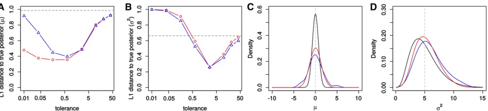
We then compared the accuracy between the two algo-rithms by calculating the total variation distance between the inferred and the true posteriors (L1 distance from kernel smoothed posterior based on 10,000 samples). We computed L1under a wide range of tolerances tofind the tolerance for which each algorithm had the best performance (i.e., minimum L1). As shown in Figure 1, A and C, ABC-PaSS produced a more accurate estimation formthan ABC-MCMC. The two algorithms had similar performance when estimatings2 (Figure 1, B and D).

The normal distribution toy model, although simple, is quite illustrative of the nature of the improvement in per-formance by using ABC-PaSS over ABC-MCMC. Indeed, our results demonstrate that the slight reduction of the summary statistics space by ignoring a single uninformative statistic when updatingmalready results in a noticeable improvement in estimation accuracy. This improvement would not be pos-sible to attain with classic dimension reduction techniques, such as partial least squares (PLS), since the information contained inxandS2is irreducible under ABC-MCMC.

Toy model 2: GLM

We expect our approach to be particularly powerful for models of the exponential family, for which a small number of sum-mary statistics per parameter are sufficient, regardless of sample size. To illustrate this, we next compared the perfor-mance of ABC-MCMC and ABC-PaSS under GLM models of increasing dimensionalityn. For all models, we constructed the design matrixCsuch that all statistics are informative for all parameters, while retaining the total information on the Figure 1 Performance to infer parameters of a normal distribution. Shown is the average over 50 chains of theL1distance between the true and

estimated posterior distributions form(A) ands2_{(B) for different tolerances for ABC-MCMC (blue) and ABC-PaSS (red). The dashed horizontal line is the}

L1distance between the prior and the true posterior distribution. (C and D) The estimated posterior distribution form(C) ands2(D) using the tolerance

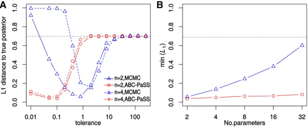
individual parameters regardless of dimensionality (see Ma-terials and Methods). For a GLM, a single linear function is a sufficient statistic for each associated parameter, and this function can easily be learned from a set of simulations, using standard regression approaches (see Theorem 2 in theAppendix). Therefore, for ABC-MCMC, we used all sta-tisticss;while for ABC-PaSS, we employedTheorem 2and used a single linear combination of statisticstiper parame-ter ui:As above, we assessed performance of ABC-MCMC and ABC-PaSS by calculating the total variation distance (L1) between the inferred and the true posterior distribu-tion. We calculated L1 for several tolerances to find the tolerance where L1 was minimal for each algorithm (see Figure 2A for examples with n¼2 and n¼4). Since in ABC-MCMC distances are calculated in the multidimensional statistics space, the optimal tolerance increased with higher dimensionality. This is not the case for ABC-PaSS, because distances are always calculated in one dimension only (Figure 2A).

We found that ABC-MCMC performance was good for low n, but worsened rapidly with increasing number of parame-ters, as expected from the corresponding increase in the di-mensionality of statistics space (Figure 2B). For a GLM with 32 parameters, approximate posteriors obtained with ABC-MCMC differed only little from the prior (Figure 2B). In contrast, performance of ABC-PaSS was unaffected by dimensionality and was better than that of ABC-MCMC even in low dimensions (Figure 2B). These results support that by considering low-dimensional parameter-specific summary statistics under our framework, ABC inference remains feasi-ble even under models of very high dimensionality, for which current ABC algorithms are not capable of producing mean-ingful estimates.

Application: Inference of natural selection and demography

One of the major research problems in modern population genetics is the inference of natural selection and demographic history, ideally jointly (Crisciet al.2012; Banket al.2014). One way to gain insight into these processes is by investigat-ing how they affect allele frequency trajectories through time in populations, for instance under experimental evolution. Several methods have thus been developed to analyze allele

trajectory data to infer both locus-specific selection coeffi-cients (s) and the effective population size (Ne). The model-ing framework of these methods assumes Wright–Fisher (WF) population dynamics in a hidden Markov setting to evaluate the likelihood of the parametersNeandsgiven the observed allele trajectories (Bollbacket al.2008; Malaspinas et al.2012). In this setting, likelihood calculations are feasi-ble, but very time-consuming, especially when considering many loci at the genome-wide scale (Follet al.2015).

To speed up calculations, Follet al.(2015) developed an ABC method (WF-ABC), adopting the hierarchical ABC framework of Bazinet al.(2010). Specifically, WF-ABCfirst estimatesNebased on statistics that are functions of all loci and then inferssfor each locus individually under the inferred value of Ne: While WF-ABC easily scales to genome-wide data, it suffers from the unrealistic assumption of complete neutrality when inferring Ne; which potentially leads to biases in the inference.

Here we show that by employing ABC-PaSS,Neand locus-specific selection coefficients can be inferred jointly, which is not possible with ABC-MCMC due to high dimensionality of the summary statistics that is a direct function of the number of loci considered.

Finding sufficient statistics: All ABC algorithms, including ABC-PaSS introduced here, require that statistics are sufficient for estimating the parameters of a given model. As mentioned above, parameter-wise sufficient statistics as required by ABC-PaSS are trivial to find for distributions of the exponential family. Since many population genetics models do not follow such distributions, sufficient statistics are known for the most simple models only. The number of haplotypes segregating in a sample, for example, is a sufficient statistic for estimating the population-scaled mutation rate under Wright–Fisher equi-librium assumptions (Durrett 2008).

For more realistic models involving multiple populations or population size changes, only approximately-sufficient statis-tics can be found. Choosing such statisstatis-tics is not trivial, however, as too few statistics are insufficient to summarize the data while too many statistics can create an excessively large statistics space that worsens the approximation of the posterior (Beaumontet al.2002; Wegmannet al.2009; Csilléry et al. 2010). Often, such statistics are thus found Figure 2 Performance to infer parameters of GLM models. (A) The average L1 distance between the

true and estimated posterior distributions for differ-ent tolerances for ABC-MCMC (blue) and ABC-PaSS (red). Solid and dashed lines are for a GLM with two and four parameters, respectively. (B) The minimum

L1 distance from the true posterior over different

tolerances for increasing numbers of parameters. (A and B) The dashed line is theL1distance between

empirically by applying dimensionality reduction techniques to a larger set of statistics initially calculated (Blum et al. 2013).

Fearnhead and Prangle (2012) suggested a method where an initial set of simulations is used tofit a linear model, using ordinary least squares that expresses each parameteruias a function of the summary statisticss:These functions are then used as statistics in subsequent ABC analysis. Thus Fearnhead and Prangle’s approach reduces the dimensionality of statis-tics space to a single combination of statisstatis-tics per parameter. However, the Pitman–Koopman–Darmois theorem states that for models that do not belong to the exponential family, the dimensionality of sufficient statistics must grow with increas-ing sample size, suggestincreas-ing that multiple summary statistics are likely required in this case as any locus carries indepen-dent information for the parameterNe:A method similar in spirit but not limited to a single summary statistic per param-eter is a partial least-squares transformation (Wegmannet al. 2009), which has been used successfully in many ABC appli-cations (e.g., Veeramahet al.2011; Chuet al.2013; Dussex et al.2014).

Here we chose to calculate the per locus statistics proposed by Follet al.(2015) and to then apply and empirically com-pare both methods to reduce dimensionality for this particu-lar model. Before dimension reduction, however, we applied a multivariate Box–Cox transformation (Box and Cox 1964) to increase linearity between statistics and parameters, as suggested by Wegmann et al.(2009). To decide on the re-quired number of PLS components, we performed a leave-one-out analysis implemented in the R package“PLS”(Mevik and Wehrens 2007). In line with the Pitman–Koopman– Darmois theorem, a small number (two) of PLS components were sufficient fors, but many more components contained information aboutNe;for which many independent obser-vations are available (Supplemental Material, Figure S1). However, thefirst PLS component alone explained already two-thirds of the total variance than can be explained with up to 100 components, suggesting that additional compo-nents add, besides information, also substantial noise. We thus chose to evaluate the accuracy of our inference with

three different sets of summary statistics: (1) a single linear combination of summary statistic for eachsandNechosen using ordinary least squares, as suggested by Fearnhead and Prangle (2012) (LC 1/1); (2) two PLS components forsand five PLS components forNe;as suggested by the leave-one-out analysis (PLS 5/2); and (3) an intermediate set of one PLS component forsand three PLS components forNe(PLS 3/1).

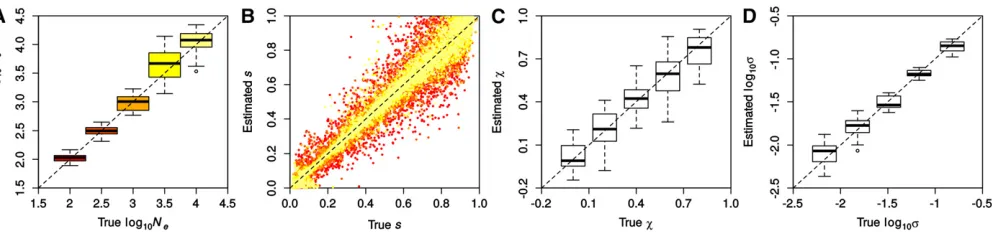
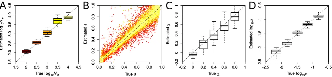
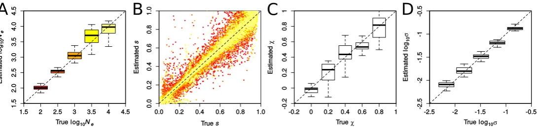
Performance of ABC-PaSS in inferring selection and de-mography: To examine the performance of ABC-PaSS under the WF model, we inferredNeandson sets of 100 loci simu-lated with varying selection coefficients. We evaluated the es-timation accuracy by comparing the estimated vs. the true values of the parameters over 25 replicate simulations, first using a single linear combination of summary statistics per parameter found using ordinary least squares (LC 1/1). As shown in Figure 3A, Ne was estimated well over the whole range of values tested. Estimates forswere on average unbi-ased and accuracy was, as expected, higher for largerNe (Fig-ure 3B). Note that since the prior onswasU½0;1;these results imply that our approach estimatesNewith high accuracy even when the majority of the simulated loci are under strong selec-tion (90% of loci hadNes.10). Hence, our method allows us to relax the assumption of neutrality on most of the loci, which was necessary in previous studies (Follet al.2015).

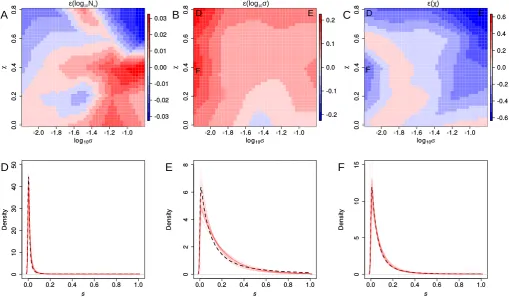
We next introduced hyperparameters for the distribution of selection coefficients (the so-called DFE). Such hyperpara-meters are computationally cheap to estimate under our frame-work, as their updates can be done analytically and do not require simulations. Following previous work (Beisel et al. 2007; Martin and Lenormand 2008), we assumed that the distribution of the locus-specificsis realistically described by a truncated GPD with locationm¼0 and parameters shapes and scalex(Figure S2).

Wefirst evaluated the accuracy of estimatingxandswhen fixing the value of the other parameter and found that both parameters are well estimated under these conditions (Fig-ure 3, C and D, respectively). Since the truncated GPD of multiple combinations of x and s is very similar, these parameters are not always identifiable. This renders the Figure 3 Accuracy in inferring demographic and selection parameters. Results were obtained with ABC-PaSS using a single combination of statistics for

accurate joint estimation of both parameters difficult (Figure S3, B and C). However, despite the reduced accuracy on the individual parameters, we found the overall shape of the GPD to be well recovered (Figure S3, D–F). Also,Newas estimated with high accuracy for all combinations ofxands(Figure S3A).

We then checked whether the accuracy of these estimates can be improved by using summary statistics of higher di-mensionality. Specifically, we repeated these analyses with a high-dimensional set (PLS 5/2) consisting of thefirstfive and thefirst two PLS components forNeand eachs, respectively, as well as a set of intermediate dimensionality (PLS 3/1) con-sisting of thefirst three PLS components forNeand only the first PLS component for eachs. Overall, all sets of summary statistics compared here resulted in very similar performance as assessed both visually (compare Figure 3,Figure S4, and

Figure S5 for LC 1/1, PLS 5/2, and PLS 3/1, respectively) and by calculating the both root mean square error (RMSE) and Pearson’s correlation coefficient between true and inferred values (Table S1). Interestingly, the intermediate set (PLS 3/1) performed worst in all comparisons, while the differences between LC 1/1 and PLS 5/2 were very subtle, particularly when uniform priors were used on alls(simulation set 1;Table S1). However, in the presence of hyperparameters ons, results were more variable (simulation sets 2–4;Table S1) and we found the effective population sizeNeto be consis-tently overestimated when using high-dimensional summa-ries such as PLS 5/2 (simulation sets 2–4;Table S1). These results suggest that while our analysis is generally rather robust to the choice of summary statistics, the benefit of extra information added by additional summary statistics is offset by the increased noise in higher dimensions. We expect that robustness of results to the choice of summary statistics will be model dependent and recommend that the performance of multiple-dimension reduction techniques should be evaluated in future applications of ABC-PaSS like we did here.

Analysis of infuenza data:We applied our approach to data from a previous study (Follet al.2014) where cultured canine

kidney cells infected with the influenza virus were subjected to serial transfers for several generations. In one experiment, the cells were treated with the drug Oseltamivir, and in a control experiment they were not treated with the drug. To obtain allele frequency trajectories of all sites of the infuenza virus genome (13.5 kbp), samples were taken and sequenced every 13 generations with pooled population sequencing. The aim of our application was to identify which viral muta-tions rose in frequency during the experiment due to natural selection and which due to drift and to investigate the shape of the DFE for the control and drug-treated viral populations. Following Follet al.(2014), wefiltered the raw data to contain loci for which sufficient data were available to calcu-late the summary statistics considered here (see Materials and Methods). There were 86 and 42 such loci for the control and drug-treated experiments, respectively (Figure S6).

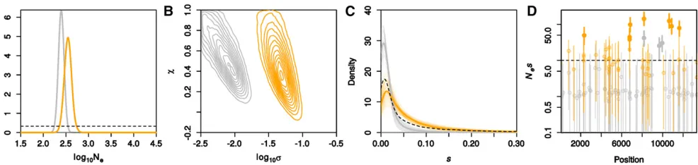
We then employed ABC-PaSS to estimateNe;sper locus and the parameters of the DFE,first using a single summary statistic per parameter (LC 1/1). We obtained a low estimate forNe(posterior medians 350 for drug-treated and 250 for control influenza; Figure 4A), which is expected given the bottleneck that the cells were subjected to in each transfer. While we obtained similar estimates for thexparameters for the drug-treated and for the control influenza (posterior me-dians 0.44 and 0.56, respectively), thesparameter was es-timated to be much higher for the drug-treated than for the control influenza (posterior medians 0.047 and 0.0071, re-spectively; Figure 4B). The resulting DFE was thus very dif-ferent for the two conditions: The DFE for the drug-treated influenza had a much heavier tail than the control (Figure 4C). Posterior estimates forNesper locus also indicated that the drug-treated influenza had more loci under strong posi-tive selection than the control (19% vs. 3.5% of loci had PðNes.10Þ.0:95;respectively; Figure 4D andFigure S6). Almost identical results were also obtained when using higher-dimensional summary statistics based on PLS com-ponents (Figure S7). These results indicate that the drug treatment placed the influenza population away from a fit-ness optimum, thus increasing the number of positively selected mutations with large effect sizes. Presumably these Figure 4 Inferred demography and selection for experimental evolution of influenza. We show results for the no-drug (control) and drug-treated influenza in gray and orange, respectively. Shown are the posterior distributions forlog_10Ne(A) andlog10sandx(B). In C, we plotted the modal DFE

mutations confer resistance to the drug, thus helping influ-enza to reach a newfitness optimum.

Our results for influenza were qualitatively similar to those obtained by Foll et al. (2014). We obtained slightly larger estimates for Ne (350vs. 226 for drug-treated and 250 vs. 176 for control influenza). Our estimates for the parameters of the GPD were substantially different from those of Follet al. (2014) but resulted in qualitatively similar overall shapes of the DFE for both drug-treated and control experiments. These results underline the applicability of our method to a high-dimensional problem. In contrast to Foll et al. (2014) who performed estimations in a three-step approach, combining a moment-based estimator forNe;ABC fors, and a maximum-likelihood approach for the GPD, our Bayesian framework allowed us to perform joint estimation and to obtain posterior distributions for all parameters in a single step.

Discussion

Due to the difficulty tofind analytically tractable likelihood solutions, statistical inference is often limited to models that made substantial approximations of reality. To address this problem, so-called likelihood-free approaches have been introduced that bypass the analytical evaluation of the likeli-hood function with computer simulations. While full-likelilikeli-hood solutions generally have more power, likelihood-free methods have been used in manyfields of science to overcome undesired model assumptions.

Here we developed and implemented a novel likelihood-free, MCMC inference framework that scales naturally to high dimensions. This framework takes advantage of the observa-tion that the informaobserva-tion about one model parameter is often contained in a subset of the data, by integrating two key innovations: First, only a single parameter is updated at a time, and the update is accepted based on a subset of summary statistics sufficient for this parameter. We proved that this MCMC variant converges to the true joint posterior distribu-tion under the standard assumpdistribu-tions.

Since simulations are accepted based on lower dimension-ality, our algorithm proposed here will have a higher accep-tance rate than other ABC approaches for the same accuracy and hence require fewer simulations. This is particularly relevant for cases in which the simulation step is computa-tionally challenging, such as for population genetic models that are spatially explicit (Rayet al.2010) or require forward-in-time simulations (as opposed to coalescent simulations) (Hernandez 2008; Messer 2013).

We demonstrated the power of our framework through the application to multiple problems. First, our framework led to more accurate inference of the mean and standard deviation of a normal distribution than standard likelihood-free MCMC, suggesting that our framework is already competitive in models of low dimensionality. In high dimensions, the benefit was even more apparent. When applied to the problem of inferring parameters of a GLM, for instance, we found our framework to be insensitive to the dimensionality, resulting in

a performance similar to that of analytical solutions both in low and in high dimensions. Finally, we used our framework to address the difficult and high-dimensional problem of infer-ring demography and selection jointly from genetic data. Specifically, and through simulations and an application to experimental data, we show that our framework enables the accurate joint estimation of the effective population size, the distribution offitness effects of segregating mutations, and locus-specific selection coefficients from allele frequency time-series data.

More generally, we envision that any hierarchical model with genome-wide and locus-specific parameters would be well suited for application of ABC-PaSS. Such models may include hyperparameters like genome-wide mutation and recombina-tion rates or parameters regarding the demographic history, along with locus-specific parameters that allow for between-locus variation, for instance in the intensity of selection, mu-tation, recombination, or migration rates. Among these, the prospect of jointly inferring selection and demographic history even from data of a single time point is particularly relevant, since it allows for the relaxation of a frequently used yet unrealistic assumption that neutral loci can be identified a priori. In addition, such a joint estimation allows for hierarchi-cal parameters to aggregate information across individual loci to increase estimation power, for instance for the inference of locus-specific selection coefficients by also jointly inferring pa-rameters of the DFE, as we did here.

Acknowledgments

We thank Pablo Duchen and the Laurent Excoffier group for comments and discussion on this work. We also thank two anonymous reviewers whose constructive criticism and comments helped to improve this work significantly. This study was supported by Swiss National Foundation grant 31003A_149920 (to D.W.).

Literature Cited

Adrion, J. R., A. Kousathanas, M. Pascual, H. J. Burrack, N. M. Haddadet al., 2014 Drosophila suzukii: the genetic footprint of a recent, worldwide invasion. Mol. Biol. Evol. 31: 3148_–3163. Aeschbacher, S., M. A. Beaumont, and A. Futschik, 2012 A novel approach for choosing summary statistics in approximate Bayes-ian computation. Genetics 192: 1027–1047.

Aeschbacher, S., A. Futschik, and M. A. Beaumont, 2013 Approximate Bayesian computation for modular inference problems with many parameters: the example of migration rates. Mol. Ecol. 22: 987–1002.

Bank, C., G. B. Ewing, A. Ferrer-Admettla, M. Foll, and J. D. Jensen, 2014 Thinking too positive? Revisiting current methods of population genetic selection inference. Trends Genet. 30: 540– 546.

Barthelmé, S., and N. Chopin, 2014 Expectation propagation for likelihood-free inference. J. Am. Stat. Assoc. 109: 315–333. Bazin, E., K. J. Dawson, and M. A. Beaumont, 2010

Beaumont, M. A., W. Zhang, and D. J. Balding, 2002 Approximate Bayesian computation in population genetics. Genetics 162: 2025–2035.

Beaumont, M. A., J.-M. Cornuet, J.-M. Marin, and C. P. Robert, 2009 Adaptive approximate Bayesian computation. Biome-trika 96: 983–990.

Beisel, C. J., D. R. Rokyta, H. A. Wichman, and P. Joyce, 2007 Testing the extreme value domain of attraction for dis-tributions of beneficialfitness effects. Genetics 176: 2441–2449. Bilodeau, M., and D. Brenner, 2008 Theory of Multivariate

Statis-tics. Springer Science & Business Media. New York, NY. Blum, M. G. B., 2010 Approximate Bayesian computation: a

non-parametric perspective. J. Am. Stat. Assoc. 105: 1178_–1187. Blum, M. G. B., M. A. Nunes, D. Prangle, and S. A. Sisson, 2013 A

comparative review of dimension reduction methods in approx-imate Bayesian computation. Stat. Sci. 28: 189–208.

Bollback, J. P., T. L. York, and R. Nielsen, 2008 Estimation of 2nes from temporal allele frequency data. Genetics 179: 497–502. Box, G. E. P., and D. R. Cox, 1964 An analysis of transformations.

J. R. Stat. Soc. B 26: 211–252.

Brown, P. M. J., C. E. Thomas, E. Lombaert, D. L. Jeffries, A. Estoup

et al., 2011 The global spread of Harmonia axyridis

(Coleop-tera: Coccinellidae): distribution, dispersal and routes of inva-sion. BioControl 56: 623–641.

Casella, G., and R. L. Berger, 2002 Statistical Inference, Vol. 2. Duxbury Press, Pacific Grove, CA.

Chu, J.-H., D. Wegmann, C.-F. Yeh, R.-C. Lin, X.-J. Yang et al., 2013 Inferring the geographic mode of speciation by contrast-ing autosomal and sex-linked genetic diversity. Mol. Biol. Evol. 30: 2519_–2530.

Cornuet, J.-M., F. Santos, M. A. Beaumont, C. P. Robert, J.-M. Marinet al., 2008 Inferring population history with DIY ABC: a user-friendly approach to approximate Bayesian computation. Bioinformatics 24: 2713–2719.

Crisci, J. L., Y.-P. Poh, A. Bean, A. Simkin, and J. D. Jensen, 2012 Recent progress in polymorphism-based population ge-netic inference. J. Hered. 103: 287–296.

Csilléry, K., M. G. B. Blum, O. E. Gaggiotti, and O. Franccois, 2010 Approximate Bayesian computation (ABC) in practice. Trends Ecol. Evol. 25: 410–418.

Durrett, R., 2008 Probability Models for DNA Sequence Evolution. Springer Science & Business Media. New York, NY.

Dussex, N., D. Wegmann, and B. Robertson, 2014 Postglacial ex-pansion and not human influence best explains the population structure in the endangered kea (Nestor notabilis). Mol. Ecol. 23: 2193–2209.

Fan, H. H., and L. S. Kubatko, 2011 Estimating species trees using approximate Bayesian computation. Mol. Phylogenet. Evol. 59: 354_–363.

Fearnhead, P., and D. Prangle, 2012 Constructing summary sta-tistics for approximate Bayesian computation: semi-automatic approximate Bayesian computation. J. R. Stat. Soc. Ser. B Stat. Methodol. 74: 419–474.

Foll, M., Y.-P. Poh, N. Renzette, A. Ferrer-Admetlla, C. Banket al., 2014 Influenza virus drug resistance: a time-sampled population genetics perspective. PLoS Genet. 10: e1004185.

Foll, M., H. Shim, and J. D. Jensen, 2015 WFABC: a Wright– Fisher ABC-based approach for inferring effective population sizes and selection coefficients from time-sampled data. Mol. Ecol. Resour. 15: 87–98.

Hernandez, R. D., 2008 Aflexible forward simulator for popula-tions subject to selection and demography. Bioinformatics 24: 2786–2787.

Jabot, F., and J. Chave, 2009 Inferring the parameters of the neutral theory of biodiversity using phylogenetic informa-tion and implicainforma-tions for tropical forests. Ecol. Lett. 12: 239–248.

Jensen, J. D., K. R. Thornton, and P. Andolfatto, 2008 An approx-imate Bayesian estimator suggests strong, recurrent selective sweeps in Drosophila. PLoS Genet. 4: e1000198.

Leuenberger, C., and D. Wegmann, 2010 Bayesian computation and model selection without likelihoods. Genetics 184: 243– 252.

Li, J., D. J. Nott, Y. Fan, and S. A. Sisson, 2015 Extending approx-imate Bayesian computation methods to high dimensions via Gaussian copula. arXiv:1504.04093.

Malaspinas, A.-S., O. Malaspinas, S. N. Evans, and M. Slatkin, 2012 Estimating allele age and selection coefficient from time-serial data. Genetics 192: 599–607.

Marjoram, P., J. Molitor, V. Plagnol, and S. Tavaré, 2003 Markov chain Monte Carlo without likelihoods. Proc. Natl. Acad. Sci. USA 100: 15324–15328.

Martin, G., and T. Lenormand, 2008 The distribution of beneficial and_fixed mutation_fitness effects close to an optimum. Genetics 179: 907–916.

Messer, P. W., 2013 SLiM: simulating evolution with selection and linkage. Genetics 194: 1037–1039.

Mevik, B., and R. Wehrens, 2007 The PLS package: principal component and partial least squares regression in R. J. Stat. Softw. 18: 1–24.

Nott, D. J., Y. Fan, L. Marshall, and S. A. Sisson, 2012 Approximate Bayesian computation and Bayes’linear analysis: toward high-dimensional ABC. J. Comput. Graph. Stat. 23: 65–86.

Ratmann, O., O. Jørgensen, T. Hinkley, M. Stumpf, S. Richardson

et al., 2007 Using likelihood-free inference to compare

evolu-tionary dynamics of the protein networks of H. pylori and P. falciparum. PLoS Comput. Biol. 3: e230.

Ray, N., M. Currat, M. Foll, and L. Excoffier, 2010 SPLATCHE2: a spatially explicit simulation framework for complex demogra-phy, genetic admixture and recombination. Bioinformatics 26: 2993–2994.

Schafer, C. M., and P. E. Freeman, 2012 Likelihood-free inference in cosmology: potential for the estimation of luminosity func-tions, pp. 3–19 inStatistical Challenges in Modern Astronomy V

(Lecture Notes in Statistics no. 902), edited by E. D. Feigelson and G. J. Babu. Springer-Verlag, New York.

Sisson, S. A., Y. Fan, and M. M. Tanaka, 2007 Sequential Monte Carlo without likelihoods. Proc. Natl. Acad. Sci. USA 104: 1760– 1765.

Veeramah, K. R., D. Wegmann, A. Woerner, F. L. Mendez, J. C. Watkinset al., 2011 An early divergence of KhoeSan ancestors from those of other modern humans is supported by an ABC-based analysis of autosomal re-sequencing data. Mol. Biol. Evol. 29: 617_–630.

Wegmann, D., and L. Excof_fier, 2010 Bayesian inference of the demographic history of chimpanzees. Mol. Biol. Evol. 27: 1425– 1435.

Wegmann, D., C. Leuenberger, and L. Excoffier, 2009 Efficient approximate Bayesian computation coupled with Markov chain Monte Carlo without likelihood. Genetics 182: 1207–1218. Wegmann, D., C. Leuenberger, S. Neuenschwander, and L. Excoffier,

2010 ABCtoolbox: a versatile toolkit for approximate Bayesian computations. BMC Bioinformatics 11: 116.

Appendix

Proof for Theorem 1. The transition kernelKðu;u9Þassociated with the Markov chain is zero ifuandu9differ in more than one component. Ifu2i¼u92ifor some indexi, then we have

Ku;u9¼piriu;u9þ12rðuÞduu9; (A1)

whereriðu;u9Þ ¼qiðu9juÞℙ

Ti¼ti;obsu9

hðu;u9Þ;duis the Dirac mass inu;and

rðuÞ ¼X n

i¼1 pi

Z

ri

u;u9du9ig:

We may assume without loss of generality that

pu9qi

uu9

pðuÞqiu9ju #1:

From (1) we conclude

ℙðs¼sobsjuÞ ¼ℙ

Ti¼ti;obsju

giðsobs;u2iÞ:

Setting

c:¼

Z

ℙðs¼sobsjuÞpðuÞdu

₂1

and keeping in mind thatu2i¼u92iandhðu9;uÞ ¼1;we get

pðujs¼sobsÞri

u;u9¼pðujs¼sobsÞqi

u9juℙTi¼ti;obsu9

h

u;u9

¼c ℙðs¼sobsjuÞpðuÞqi

u9juℙTi¼ti;obsu9

_pu9qiuu9

pðuÞqiu9ju

¼c ℙTi¼ti;obsju

giðsobs;u2iÞℙ

Ti¼ti;obsu9

p

u9qi

uu9

¼c ℙTi¼ti;obsu9

gi

sobs;u92i

ℙTi¼ti;obsju

p

u9qi

uu9

¼c ℙs¼sobsu9

ℙTi¼ti;obsju

p

u9qi

uu9hu9;u

¼p

u9js¼sobs

ri

u9;u:

From this and Equation A1 it follows readily that the transition kernelKð;Þsatisfies the detailed balanced equation

pðujs¼sobsÞK

u;u9¼pu9s¼sobs

Ku9;u

of the Metropolis–Hastings chain.

h

Suppose that, given the parametersu;the distribution of the statistics vectorsis multivariate normal according to the GLM

s¼cþCuþe;

wheree N ð0;SsÞand for anym3nmatrixC:If the prior distribution of the parameter vector isu N ðu0;SuÞ;then the

posterior distribution ofugivensobs is

with D¼ ðC9S2s1CþS2 1

u Þ2

1

andd¼C9S2s1ðsobs2cÞ þS2_u1u0 (see, e.g., Leuenberger and Wegmann 2010). We have the following:

Theorem 2.Letcibe the ith column ofCandbi¼S2 1

s ci:Moreover,let

ti¼tiðsÞ ¼b9is:

Thentiis sufficient for the parameteruiand the collection of statistics

t¼ ðt1;. . .;tnÞ9

yields the same posterior(A2)ass:

In practice, the design matrixCis unknown. We can perform an initial set of simulations from which we can infer that

Covðs;uiÞ ¼VarðuiÞci:

A reasonable estimator for the sufficient statistictiis then^ti¼bb9iswith

^

bi¼S^2s1S^sui; (A3)

whereS^sandS^suifori¼1;. . .;nare the covariances estimated, for instance, using ordinary least squares.

Proof for Theorem 2. It is easy to check that the mean oftiismi¼t9iðCuþcÞand its variance iss2i ¼ti9Ssti9:The covariance betweensandtis given by

Sst¼Eððs2Cu2cÞðti2miÞÞ

¼Eðee9tiÞ ¼Ssti

Consider the conditional multinormal distributionsjti:Using the well-known formula for the variance and the mean of a conditional multivariate normal (see,e.g., Bilodeau and Brenner 2008), we get that the covariance ofsjtiis given by

Ssjt¼Ss2si22SstS9st

and thus is independent ofu:The mean ofsjtiis

msjt¼Cuþcþs2i2Sstti9ðs2Cu2cÞ:

The part of this expression depending onuiis

I2Sstiti9 ti9Ssti

ciui:

Insertingti¼S2 1

s ciwe obtain

 ci2SsS

21

s cici9S2s1ci ci9S2s1SsS2s1ci

!

ui¼ ðci2ciÞui¼0:

Thus the distribution ofsjtiis independent ofuiand hencetiis sufficient forui:

To prove the second part ofTheorem 2, we observe thattis given by the linear model

t¼C9S2_s1s¼C9S_s21CuþC9S2_s1cþh

withh¼C9S2s1e:Using CovðhÞ ¼C9S2 1

s Cwe get for the posterior variance

C9S2_s1

C9S2_s1C

₂1

C9S2_s1CþS2_u1

₂1

¼C9S2_s1CþS2_u1

₂1

¼D:

Similarly we see that the posterior mean isDd:

GENETICS

Supporting Information www.genetics.org/lookup/suppl/doi:10.1534/genetics.116.187567/-/DC1

Likelihood-Free Inference in

High-Dimensional Models

Athanasios Kousathanas, Christoph Leuenberger, Jonas Helfer, Mathieu Quinodoz, Matthieu Foll, and Daniel Wegmann

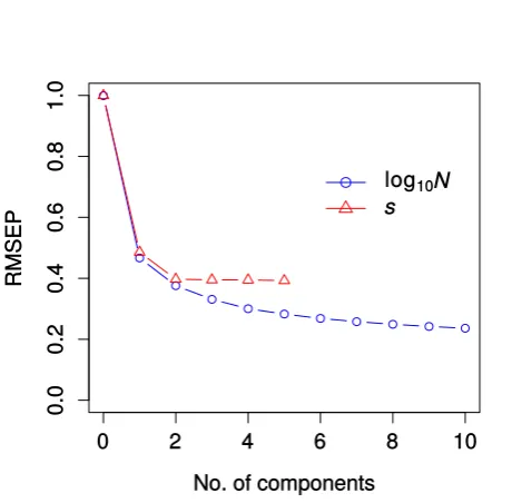
Figure S1: Prediction error for partial least squares analysis (PLS). The root mean squared prediction error (RMSEP) is shown for parametersNe and sas a function of increasing number

L

σ

χ

s

l

N

e

ξ

l

F

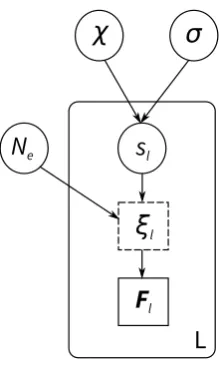
l

Figure S2: Directed acyclic graph describing the Wright-Fisher model examined in this study. Solid circles represent parameters to be estimated. The dashed square represents the full data, which is summerized here by a vector of statistics Fl, indicated by a solid square. Nodes

A

B

C

D

E

F

D E

F F

D E

ε(log10Ne) ε(log10σ) ε(χ)

Figure S3: Accuracy in estimating Ne and DFE parameters σ and χ jointly. (A,B,C)

Sets of simulations of 100 loci were conducted for combinations of parametersσandχ over a grid

from their prior range and we evaluated the median approximation error (=estimate-true) over 25

replicates. Color gradients indicate the extent of overestimation (red) or underestimation (blue) of each parameter. These results suggest very high accuracy when estimatingNewith maximum

≈0.04or 1% of the prior range and rather low forσ(about 10% of the prior range). In contrast, is rather large forχ, spanning up to 75% of the prior range. This is due to several combinations

ofχ and σleading to very similar shapes of the truncated GPD. This is illustrated in panels D,

A

B

C

D

Figure S4: Accuracy in inferring demographic and selection parameters using the PLS 5/2 set of statistics. Results were obtained with ABC-PaSS using ve and two PLS components forNeand eachs, respectively (PLS 5/2). Shown are the true versus estimated posterior medians

for parameters Ne (A), s per locus (B), χ and σ of the Generalized Pareto distribution (C and

D, respectively). Boxplots summarize results from 25 replicate simulations, each with 100 loci. Uniform priors over the whole ranges shown were used. (A, B):Ne assumed in the simulations is

represented as a color gradient of red (lowNe) to yellow (highNe). (C,D): Parameters µandNe

A

B

C

D

Figure S5: Accuracy in inferring demographic and selection parameters using the PLS 3/1 set of statistics. Results were obtained with ABC-PaSS using three and one PLS components forNeand eachs, respectively (PLS 5/2). Shown are the true versus estimated posterior medians

for parameters Ne (A), s per locus (B), χ and σ of the Generalized Pareto distribution (C and

D, respectively). Boxplots summarize results from 25 replicate simulations, each with 100 loci. Uniform priors over the whole ranges shown were used. (A, B):Ne assumed in the simulations is

represented as a color gradient of red (lowNe) to yellow (highNe). (C,D): Parameters µandNe

were xed to 0 and103_{, respectively,log}

A

B

C

D

Figure S6: Allele trajectories (A, C) and posterior estimates forNes(B, D) for control

A

B

C

D

Figure S7: Inferred demography and selection for experimental evolution of Infuenza using the PLS 3/1 set of statistics. We show results for the no-drug (control) and drug-treated Inuenza in grey and orange, respectively. Shown are the posterior distributions for log10Ne (A) andlog10σ andχ(B). In panel C, we plotted the modal distribution of tness eects (DFE) with thick lines

by integrating over the posterior of its parameters. The thin lines represent the DFEs obtained by drawing 100 samples from the posterior ofσandχ. Dashed lines in panels A and C correspond to

the prior distributions. In panel D, the posterior estimates forN esper locus versus the position of

Simulation set Parameter Method RMSE Pearsons R2

Set 1

s

LC 1/1 0.0700 0.970

PLS 3/1 0.0809 0.960

PLS 5/2 0.0743 0.966

log10(Ne)

LC 1/1 0.178 0.969

PLS 3/1 0.199 0.962

PLS 5/2 0.171 0.972

Set 2

s

LC 1/1 0.0191 0.954

PLS 3/1 0.0390 0.957

PLS 5/2 0.0195 0.953

log10(Ne)

LC 1/1 0.0292

-PLS 3/1 0.0390

-PLS 5/2 0.0485

-χ

LC 1/1 0.126 0.911

PLS 3/1 0.127 0.910

PLS 5/2 0.140 0.895

Set 3

s

LC 1/1 0.0226 0.987

PLS 3/1 0.0228 0.986

PLS 5/2 0.0227 0.986

log10(Ne)

LC 1/1 0.0427

-PLS 3/1 0.189

-PLS 5/2 0.374

-log10(σ)

LC 1/1 0.0783 0.988

PLS 3/1 0.0776 0.989

PLS 5/2 0.0844 0.984

Set 4

s

LC 1/1 0.0258 0.982

PLS 3/1 0.0259 0.981

PLS 5/2 0.0254 0.981

log10(Ne)

LC 1/1 0.0577

-PLS 3/1 0.0889

-PLS 5/2 0.351

-log10(σ)

LC 1/1 0.0191 0.961

PLS 3/1 0.0180 0.968

PLS 5/2 0.0167 0.968

χ

LC 1/1 0.306 0.667

PLS 3/1 0.306 0.659

PLS 5/2 0.291 0.666

Table S1: Performance of ABC-PaSS coupled with dierent dimension reduction tech-niques in Wright-Fisher simulations. We computed the root mean square error (RMSE) and Pearson's correlation (R2_{) between true and estimated parameter values using three dierent} di-mension reduction strategies: a single linear combination per parameter calculated according to Theorem 2 (LC 1/1), three and one PLS components for parameterslog10Ne ands, respectively

(PLS 3/1), and ve and two PLS components for parameters log10Ne and s, respectively (PLS

5/2). Results shown are for four sets of 25 replicate simulations: Set 1 assumed uniform priors for

Neands(U[0.5,4.5]andU[0,1], respectively), Sets 2-4 assumed a generalised pareto distribution

forswith hyperparamersσ andχ. For Set 2 we varied χ(U[−0.2,1]) and keptσxed (= 0.01),

for set 3 we variedlog10σ (U[−2.5,−0.5]) and kept χ xed (= 0.5) and for Set 4 we varied both

σand χ. For Sets 2-4 we performed simulations only for log10Ne = 3, thus R2 is not calculable