ABSTRACT
NIX, ANISHA MAHESH. Investigating the Links Among Stereotypes, Self-Image, and Career Commitment to the Sciences. (Under the direction of Mary B. Wyer).
Women have historically been underrepresented in the science, technology, engineering, and mathematics (STEM) fields. One reason for this continued
underrepresentation might be existing stereotypes of STEM fields, as well as the lack of historical role models within these fields. A longitudinal analysis conducted over a one-semester period in an introductory Chemistry course was conducted to explore the effects of a curriculum intervention that introduced the contributions of women to chemistry on students’ stereotypes about STEM fields, self perceptions, and their commitment to STEM fields.
Investigating the Links Among Stereotypes, Self-Image, and Career Commitment to the Sciences
by
Anisha Mahesh Nix
A thesis submitted to the Graduate Faculty of North Carolina State University
in partial fulfillment of the requirements for the degree of
Master of Science
Psychology
Raleigh, North Carolina 2009
APPROVED BY:
_______________________________ ______________________________
Dennis O. Gray Shevaun Neupert
DEDICATION
This work is dedicated to my family. To my mother, whose support and guidance have been invaluable in my education and my life. To my father, who has always believed in my ability to achieve any goal. To my husband, whose love and support have made it possible for me to achieve this particular goal.
BIOGRAPHY
Anisha Nix was born in India, where she spent the first nine years of her life. Upon relocating with her family to the U.S., she spent most of the remainder of her childhood and adolescence in Grayslake, IL. She attended Virginia Polytechnic Institute and State
University and graduated in December, 2005 with a Bachelor of Science in Psychology and a Bachelor of Arts in Spanish. She went on to attend graduate school at North Carolina State University, where her primary research interest was the underrepresentation of women in the sciences.
ACKNOWLEDGMENTS
I would like to acknowledge the many people who have been instrumental in the completion of this project. First, I would like to thank my advisor, Mary Wyer, who has unwaveringly supported me through numerous changes and edits and whose guidance has helped me navigate the maze of graduate school for the past three years.
I would also like to thank my other committee members, Dennis Gray and Shevaun Neupert, who have provided me with insightful questions, thoughtful answers, and a push in the right direction.
I am indebted to my peers in the Stereotypes lab, both past and present, who have shown me the ropes and have been there through the setbacks and celebrations of this process.
This project could not have been carried out without Maria Oliver-Hoyo and Ana Ison, of the Chemistry department, who were invaluable in the creation of the intervention and in the data collection process.
TABLE OF CONTENTS
LIST OF TABLES ...vii
LIST OF FIGURES...viii
INTRODUCTION... 1
LITERATURE REVIEW ... 2
Career Development ... 2
Attrition and Persistence in STEM Majors ... 10
Self Concept ... 13
Gender and Occupational Stereotypes ... 14
Stereotype Threat... 20
Difference in Interests... 22
Past Interventions ... 24
PURPOSE OF STUDY ... 26
METHOD ... 28
Research Design ... 28
Setting and Population ... 28
Procedures ... 29
Survey Instrument... 31
RESULTS ... 33
Stereotypes of Scientists ... 34
Fit Score ... 42
Group Differences in Fit ... 43
Fit and Career Commitment ... 43
Effects of Gender... 45
Exploratory Analyses... 50
Major... 51
Self Image... 57
Individual Level Beliefs about Scientists... 58
DISCUSSION ... 61
Major Results ... 63
Limitations ... 66
Conclusions and Implications ... 67
Future Directions ... 69
REFERENCES... 71
APPENDICES ... 83
Appendix A: In-Class Modules ... 84
Appendix B: Online Modules... 90
Appendix C: Careers in Science Survey ... 98
Appendix D: Intervention Timeline... 118
LIST OF TABLES
Table 1. Items on Stereotypes of Scientists Scale... 35
Table 2. Exploratory Factor Analysis Results for Observations of Scientists Scale, Time 1... 40
Table 3. Exploratory Factor Analysis Results for Career Commitment Scale, Time 1... 44
Table 4. Analysis of Variance Results, Gender... 48
Table 5. Hierarchical Regression Results... 50
Table 6. Analysis of Variance Results, Major... 56
Table 7. Analysis of Variance Results, Total Fit Score... 60
LIST OF FIGURES
Figure 1. Fit Scores by Time and Gender... 47
Figure 2. Career Scores by Major, Time 1... 52
Figure 3. Career Scores by Major, Time 2... 53
Figure 4. Career Scores by Major and Gender, Time 1... 54
Figure 5. Career Scores by Major and Gender, Time 2... 55
Introduction
According to statistics from the National Science Foundation (2006), women earned 42.6% of all Bachelor's degrees that were awarded in 1966. By 2004, women were earning over half the Bachelor’s degrees in all fields combined, with 57.6% percent of all degrees being awarded to women. Despite this overall growth in women’s
educational attainment, there are still dramatic discrepancies in the degrees earned by men and women by field.
In some fields, women have been on the higher end of the degree earning
spectrum, with 40% of Psychology Bachelor’s degrees going to women in 1966 and over 77% in 2004. There is similar growth in the agricultural and biological sciences, with 25% of Bachelor’s degrees awarded to women in 1966 and over 60% in 2004 (NSF, 2006).
Chemistry, where men and women have reached equity in undergraduate degree earning, women are underrepresented at higher level degrees, earning just 31% of PhDs as
compared with 51% of Bachelor’s degrees in 2004. Though the uneven pattern across fields has been apparent for decades, the reasons for it are not. This paper focuses on four factors that are suggested by major theoretical and empirical approaches: (1) career development, (2) stereotypes about science and mathematics, (3) self-image, and (4) stereotypes about gender.
Literature Review
Career 1Development
One of the most basic ideas in the career counseling literature is that there must be some level of congruence between a worker’s personal characteristics and the career’s requirements. Without this congruence, outcomes such as attrition, low job satisfaction, and low commitment are more likely (Ployhart, Weekley, & Baughman, 2006).
Holland’s Career Theory introduces the idea that individuals make decisions by matching their personal characteristics with the characteristics that they believe are needed in that occupation (Holland, 1997). Holland came up with a catalogue of different personality types as determined by personal characteristics. He then matched those personality types to the type of environment found in various occupations. In order to maximize constructs such as job satisfaction and performance, he theorized that individuals should enter fields
that fit their personality type. Although Holland did not focus specifically on STEM, his work suggests the pivotal idea that in order to have a productive and fulfilling work experience, there should first be a high degree of congruence between one’s self-concept regarding work-related characteristics and one’s perceptions about what characteristics are needed to do that work.
Super’s Vocational Theory (Super, Savickas, & Super, 1996) also emphasizes the need for congruence between individual and occupational characteristics. However, Super et al.’s focus examined this congruence in the context of life stages. They theorized that individuals’ career trajectory must match their life trajectory in terms of maturation and family and personal commitments. Thus, Super et al. suggest that career progression is reflected by individuals’ plans for their personal lives.
Most career development theories see career decision-making as a narrowing of interests that occurs in relation to maturation (Brown & Brooks, 1996; Oyserman, Grant, & Ager, 1995). However, most of these theories were constructed by studying the career trajectories of men, so their applicability to women is unclear. It has been suggested that women and men have different occupational opportunities and that women’s
The idea of possible selves plays a large role in the career decision making
process of women. The term “possible selves” refers to the idea that individuals visualize themselves in various careers when making decisions about careers; possible selves are shaped by interactions and experiences during adolescence and early adulthood
(Pizzolato, 2006). Since this is also the time during which career interests are beginning to be strengthened, possible selves have a rather substantial influence on career decision making. Peer influences have been found to be important in shaping possible selves, and since gender is extremely salient in terms of group membership, it is reasonable that gender identity is vital during the formulation of an individual’s possible selves (Pizzolato, 2006).
In addition to visualizing their career itself, individuals also picture how that career will shape their outside life. While choosing a career involves examination of one’s goals and aspirations, it might be a more complex process for women. Since women have traditionally been responsible for a larger portion of the housekeeping and child rearing tasks, they might be more inclined to avoid or leave an occupation if they feel that they will not be able to devote sufficient time or energy to these tasks. Women who place high importance on family roles are more likely to move from a gender non-traditional career, such as STEM careers, to a non-traditional career, such as teaching or nursing (Sax & Bryant, 2006). Haber (1980) found women who were pursuing
immediate career saw themselves as being less feminine than did women who were majoring in a field that was based in academia and required further study, such as an undergraduate or graduate education, prior to entering a profession (Wulff & Steitz, 1997).
Patterns in women’s home lives also come into play when women are making career decisions. Beginning in the mid to late twenties, women’s home commitment is negatively related to their career commitment, but men’s levels of home and career commitment do not show this same pattern (Farmer, 1997; Farmer, Wardrop, &
Anderson, 1995). Thus, there’s some evidence that women might feel that they have to choose between being more committed at home or at their job, whereas men do not feel this pressure. Moreover, working mothers report feeling both stress and guilt in trying to balance their personal and professional lives (Guendouzi, 2006). This phenomenon suggests that women’s role as caretaker is so engrained in societal attitudes that when they choose to fulfill outside interests, such as a career, they feel that they are somehow doing a disservice to their role as a mother, wife, or family member. Thus, even though women may be highly talented in STEM fields, if they believe that a STEM career is incompatible with their other personal goals, they are forced to compromise either their career or personal goals.
fairly consistent, they placed greater value on autonomy at the end of the three year period (Madill, Montgomerie, & Stewin, 2000). This indicates that early in women’s college experience, they begin to see themselves more as individuals. Lips (2004) found that women’s current and possible selves in high school are fairly congruent, whereas by college, women’s future selves are more gender constrained than their current selves, which indicates that they see themselves as being more constrained by gender roles in the future than in the present. Moreover, high school women are more likely than college women to see a high powered career as being a possibility for them. Thus, in addition to a narrowing of interests, women’s occupational choice process is also affected by their perceptions of gender roles as they mature, both in terms of their career and their personal lives.
Neither Holland nor Super specifically addresses the influence of demographic variables such as gender on their theories. However, gender plays an important role in shaping the constructs that Holland and Super considered in their theories. Holland focuses heavily on self-concept, which is influenced by social relationships and patterns of reinforcement and experiences (Rogers, 1947; Purkey, Raheim, & Cage, 1983). Since children from a very young age are exposed to differential experiences and reinforcement based on gender, self-concept is tied to gender (Martin & Ruble, 2004).
Gender can also be applied to Super’s theory, as it deals with life experiences and stages. Although men and women take on more equal roles at home now than they have in the past, on average, women are still responsible for more of the homemaking and childrearing duties than are men (Baxter, Hewitt, & Haynes, 2008). Therefore, women’s life experiences and stages are different from those than men undergo.
Career outcomes such as job performance, job satisfaction, and career
commitment have all been linked to how well one’s career of choice fits his or her needs, interests, and personality (Ployhart, Weekley, & Baughman, 2006). Individuals who are undergoing the process of choosing a career rely on their own perceptions and
their perceptions of the requirements and environment within various careers (Holland, 1997).
Gender complicates the career choice process, as men and women are likely to consider different career options because of their perceptions of what is required within various careers. While aptitude for math has been linked to entry into STEM fields, Hollinger (1985) found that self-perceptions about math ability alone are not adequate predictors of whether women enter STEM fields. Self-perceptions about such personality characteristics as friendliness and creativity, as well as perceptions about one’s
mechanical and manual ability are all important in predicting entry into gender non-traditional careers. Thus, a change in self-perceptions might result in a drastic change in career choice.
In addition to self-perceptions, perceptions about the environment within their future career might also influence women’s career decision-making. Role modeling and individual assistance and encouragement, especially by female instructors, positively influence women’s decisions in science and engineering (Madill, Ciccocioppo, Stewin, Armour, & Montgomerie, 2004). Since individuals rarely have the opportunity to see a career as an “insider” before deciding to enter it, they rely on experiences of other individuals who are already working in various fields. Madill et al. suggest that the availability of female role models allows women who are making career related decision to explore such factors as family-friendliness, amount of education needed, or
Finding individuals who are similar to themselves in the field of their choice who can serve as a mentor often bolsters individuals’ career persistence (Subotnik & Steiner, 1993). Women who left the sciences mentioned that they were not able to find a suitable female mentor in college, which contributed to their decision to enter a different field. Conversely, many of those who stayed in the sciences reported that they had one or more female mentors who provided them with professional support and introductions to important people in the field. Furthermore, while role models and mentors in general are related to more positive outcomes, there is evidence suggesting that the positive or negative nature of the mentoring relationship can also be influential. More positive mentoring experiences are related to higher level career aspirations, especially in women who already have high career choice self-efficacy (Nauta, Epperson, & Kahn, 1998).
In addition to the lack of contemporary mentors, another issue within STEM fields is the lack of historical female role models. Since work within these fields has historically been done by men, female students are not exposed to female scientists who have done similar work; this is especially true because historically, work that has been done by women has been misrepresented as having been done by men (Derrick, 1982). Furthermore, there is often a lack of personal information about both men and women within these courses, as it is expected that the science that is taught will stand on its own merit. The lack of humans and human experiences within the course material might be detrimental to women’s learning process (Rosser, 1990), thus further encouraging them to avoid or leave the field.
Attrition and Persistence in STEM Majors
rapid rate than women’s levels of the same constructs (Farmer, Wardrop, & Anderson, 1995).
One of the key predictors of persistence in STEM fields is congruence between one’s interests and characteristics and the interests and characteristics of a given
discipline (Schaefers, Epperson, & Nauta, 1997). Thus, if there are gendered patterns of attrition from STEM fields, there may also be gendered patterns in the congruence of self perceptions and perceptions of the field of study.
Parental support of non-traditional careers, or careers that have historically been largely occupied by men, has also been linked to both persistence and attrition of women in STEM majors. Parental support has been found to be one of the most important predictors of both self-efficacy and career choice, especially for non-traditional careers (Flores & O’Brien, 2002; Turner, Steward, & Lapan, 2004), but it does not specifically influence interest in the sciences (Quimby, Wolfson, & Seyala, 2007). Thus, it would seem that parents can provide the necessary support to encourage their daughters to consider non-traditional careers in general, rather than science-specific careers.
In addition to perceptions of a field that are gathered via mentoring relationships and general stereotypes about gendered occupations, they are also based on individuals’ experiences within that field. Women who left engineering, for example, reported a more negative environment than those who persisted in the field (Schaefers, Epperson, & Nauta, 1997). Thus, if women are faced with the challenges of majoring in a
nontraditional field and they have negative perceptions of the environment, they might be even less likely to persist than women who face similar challenges, but who perceive the same environment as being less negative. Women who leave STEM programs also often report that one of their primary reasons was the isolation that they felt in the competitive, isolative culture of the sciences (Madill, Montgomerie, & Stewin, 2000).
There is also evidence that women’s value systems play a role in whether they will persist in a given field. Women who move from a gender traditional to a gender non-traditional field during college tend to place greater value on status and have more liberal views on human behavior than those who stayed in or moved to a gender traditional field (Sax & Bryant, 2006).
Self-Concept
Gender and Occupational Stereotypes
Occupational stereotypes also often interact with gender stereotypes, and this interaction places women at a disadvantage. In the professional context, the ideal person is described as being autonomous and agentic, both of which are considered masculine traits, while in the private sphere, traits such as being more communal and personally attractive were emphasized (Echabe & Castro, 1999). Thus, in the workplace in general, men are seen as being closer to the ideal, and therefore, more successful.
From a very young age, children are socialized to display gender appropriate behaviors. They learn these behaviors in two primary ways: by observation and by more direct instruction or encouragement (Martin & Ruble, 2004). Beginning in infancy, children are able to distinguish men and women based on physical appearance and pitch of voice (Patterson & Werker, 2002). Moreover, parents often surround children with gender appropriate toys, clothing, etc from birth. The presence of these cues sends messages to children about how they should behave. Once they understand which gender group they themselves belong to, they are then able to imitate other individuals of that same gender (Martin & Ruble, 2004).
Children’s stereotypes about gender are formed early in development.
a given situation. However, stereotypes can be highly inaccurate as their function is to categorize individuals and situations based on superficial cues. Since children’s stereotypes about gender are developing at the same time as their gender identity, their stereotypes about gendered behaviors and interests influence whether they develop those behaviors and interests (Leinbach, Hort, & Fagot, 1997; Martin & Ruble, 2004). Gender identity is composed of internalized stereotypes, as well as external expectations for behavior. Internalized stereotypes become part of one’s self-concept, while certain external expectations are powerful enough to influence one’s choices. Thus, stereotypes function in multiple ways to determine behavior (Echabe & Castro, 1999).
In the early grades, parent perceptions of children’s ability serve as a better predictor of children’s grades than the children’s own self perceptions. Furthermore, parent perceptions tend to be dictated by gender stereotypes, even if evidence of their children’s performance does not support those stereotypes (Frome & Eccles, 1998). School-aged children’s gendered behaviors, however, are no longer reinforced only by parents, but also by peers and teachers. The idea, for example, that women lack talent or aptitude for math and science, is found as early as elementary school (Steele, 2003).
Children also show a sharp division in future aspirations. Even at age 6, children are more likely to say that they desire and would have a higher chance of success at a gender traditional career (Auger, Blackhurst, & Wahl, 2005). These ideas about which professions are appropriate for men and women continue throughout childhood
about novel jobs given some information about people who generally work that job (Shepelak, Ogden, & Tobin-Bennett, 1984). Moreover, these gender stereotypes are complex and contain information not only about which gender is appropriate for the job, but also about gender based sanctions that people of the opposite gender would face if they attempted to enter that profession. Thus, children are aware at a young age not only that there are professions that are appropriate for them based on gender, but also that if they attempt to cross gender lines in a professional context, there would be negative consequences to face 2(Shepelak, Ogden, & Tobin-Bennet, 1984).
Gender also shapes career choice via gender differences in values in human relationships. As early as grade 4, a difference can be seen in the values that boys and girls place on social behaviors. Boys endorse being more competitive, aggressive, and independent, while girls endorse being more compliant and dependent (Lupaschuk & Yewchuk, 1998). Thus, from an early age, women self select to enter fields which are perceived to present a better fit for compliance and dependence, while men plan for fields that are perceived to require competitiveness and independence. Girls and women are also told to choose a career that would make them happy, whereas boys and men are given the message that they should choose a career that will allow them to maximize their
2
earning potential (Madill, Montgomerie, & Stewin, 2000). Thus, from a very young age, boys are encouraged to enter careers that will promote financial success, while girls are encouraged to consider careers based on personal, rather than financial considerations.
Women’s beliefs about the roles that men and women should ideally hold also influence their career decisions. Students who have more egalitarian gender roles, or who believe that women and men should be of equal status, also have higher levels of career decision making self-efficacy (Gushue & Whitson, 2006) and women who choose more traditional careers hold more traditional gender attitudes than those who choose non-traditional careers (Murrel, Frieze, & Frost, 1991). Furthermore, women who hold more egalitarian gender attitudes are more likely to want to earn an advanced degree and to want a job that would allow them financial as well as advancement benefits (Colaner & Warner, 2005).
One meta-analysis found that gender differences in math self-efficacy increased as students progressed through high school and college, suggesting that stereotypes about gender and science might become more salient during this time period (Hyde, Fennema, Ryan, Frost, & Hopp, 1990). This might help explain why there is considerable attrition of women from the sciences as they enter and progress through college. This pattern persists and worsens at higher degree levels, with women earning a greater portion of the STEM degrees at the undergraduate level than at the graduate level (NSF, 2006).
being masculine, such as science and engineering, are seen as being more independent and less cooperative. They found also that individuals who worked in these masculine fields tend to see themselves as possessing the stereotypical characteristics associated with the occupation. Since learning has both academic and social components, if individuals lack the social support necessary in order to learn and pursue a career in science, they are less likely to persist in their aspirations. The identity that women take on as scientists must be compatible both with the science community and the cultural
community to which they belong (Brickhouse & Potter, 2001).
If women are reinforced for being communal and cooperative, they are more likely to believe that their personal characteristics do not match the characteristics that are prevalent in traditionally male fields. Keith and Cardador (2007) were able to categorize cognitions about science and technology into eight groups, one of which was agreement between an internalized image of scientists and self perceptions. They concluded that if there were a greater agreement between the internalized image of a scientist and an individual's self perceptions, the individual would be more likely to view science in a positive light and to participate in a science-related career. This suggests that if the fit between one’s stereotypes of STEM and self-perceptions is better, the individual would more likely choose and be committed to a STEM career.
In addition to the lack of congruence between stereotypes about women’s
held not only outside, but also within the STEM fields and women in STEM find themselves needing to work much harder than men in order to be judged as being competent (Foschi, 1996).
Although there is an idealized image of women being able to “have it all,” women are actually more likely to choose either career or family orientation and focus their efforts on the domain of their choice. One 1992 study found that by age 26, only 15% of women had combined high career aspirations or achievement with parenting, and women who had been higher in academic achievement as adolescents were more likely to be career as opposed to family oriented (Gustafson, Stattin, & Magnusson, 1992). Female college students who view their future work environment as being more equitable are more committed to their future careers and have greater career aspirations than women who stated that they expected negative outcomes based on gender in their field of choice (Farmer, 1997). Thus, if women have the stereotype that STEM fields are less family friendly, they may have lower career commitment, as well as lower career aspirations for STEM fields. Furthermore, parental input regarding women’s roles can also shape women’s career commitment. Career commitment is higher for women whose mothers emphasize their role as a career woman, regardless of whether these mothers also
emphasize family roles, whereas for women whose mothers emphasize family roles at the expense of career roles, career commitment is relatively low (Haber, 1980).
in STEM fields during the socialization process due to the stereotype that girls are not interested in computers and other forms of technology. Adya and Kaiser (2005), who compiled past research in order to create an explanatory model for women's career choices in the technology field suggest that early access to computer decreases the level of intimidation caused by technology and that same sex education might reduce bias against the technology field.
Stereotype Threat
In order to understand why even highly talented women leave STEM fields at higher rates than men, it is important to understand how gender-related stereotypes affect women's self-perceptions of performance. Steele and Aronson (1995) suggest that salient characteristics that differentiate individuals’ status based on demographic variables alter their expectations about relevant situations and that aspirations in turn are affected by expectations; one such demographic variable is gender (Correll, 2004). For example, if women are told that their characteristics are incompatible with a certain task, they will expect to be less likely to aspire to complete that task as they will have lower
expectations of success. This phenomenon is known as stereotype threat.
Furthermore, women who are more aware of belonging to a stigmatized group are more affected by negative stereotypes about that group than those who do not consider themselves part of a stigmatized group (Brown & Pinel, 2003). When women are in a group that contains more men, stereotype threat for gender is more prevalent (Inzlicht & Ben-Zeev, 2000). Thus, it is possible that in STEM fields that contain more men and in which the presence and accomplishments of women is downplayed, female students feel more threatened by their gender.
Stereotype threat is especially insidious because it makes women feel that they are not capable of accomplishing the tasks and meeting the challenges that are present in the STEM fields. In addition to simply making gender a salient self-characteristic, stereotype threat also raises the idea that performance on a task or in a subject is dependent on some innate trait associated with one’s gender. As a result, individual variance is downplayed and the importance of a group characteristic is overestimated. Undergraduate women in STEM fields report experiencing greater levels of stereotype threat and gender
discrimination than women in more gender traditional fields (Steele, James, & Barnett, 2002). This suggests that for women in STEM, gender is a more salient
self-characteristic in their day-to-day academic lives than it is for women in gender traditional fields and moreover, that it is a self-characteristic that is linked to lower performance.
than did men; however, when gender was not made salient, women and men set similar standards of success. Thus, women feel that they have to work harder to achieve success if they are considering their gendered identity, but not otherwise.
Difference in interests
James (1993) suggested that one reason why more women and people of color do not enter the sciences is because there is a disconnect between their attitudes and values and the attitudes and values that are prevalent in science. Theorists in feminist science studies have pointed to the predominance of white male scientists as influential in education, employment, and the content of STEM disciplines (Keller, 1982; Rosser, 1990). The questions asked and methods used to investigate those questions have largely excluded or marginalized the education, experiences, and interests of women and people of color (Boxer, 1998).
Teachers also reinforce male and female students in different ways (Sheridan & Henning-Stout, 1994). Males get more opportunity to practice abstract reasoning, while females are often asked questions that require recitation of fact (Morse & Handley, 1985). While it might seem that females are thus favored by teachers, this practice actually has a detrimental effect, as it reinforces the stereotype that females are unable to understand difficult material.
More positive feedback regarding performance has been linked to more positive self assessment of ability, but there is a gender effect as well, as males are more likely to have a positive self assessment of ability than females, even when they receive the same feedback (Correll, 2001). Conversely, women also are assessed more strictly in math and science and therefore must display higher levels of performance in order to achieve the same rating of competence that men get at lower performance levels (Foschi, 1996). Thus, gender differences in self image in math and science emerge from gender differences in perceptions of performance that exist regardless of actual performance.
In feminist theory about STEM, such characteristics as objectivity, rationality, and competitiveness are valued in STEM fields and in academia in general. However, these are characteristics that are stereotypically associated with men. Theorists argue that women, in contrast, are seen as being subjective, emotional or intuitive, and cooperative (Keller, 1982). In order to fit into the STEM fields, women must take on the
By the logic of this argument, if women see themselves as being cooperative and valuing situations in which they are able to work with a group of individuals, then they will see a disconnect between their personal characteristics and the environment that is stereotypical of STEM fields. This might cause women to avoid such fields altogether, as they believe that they do not possess the appropriate characteristics to succeed in the field.
In response to this argument, some scientists have asserted that science will be more attractive to women and minority students if it is presented as a process, rather than as an end result (Brickhouse, Carter, & Scantlebury, 1990; Rosser, 1990). In this
approach, scientists are not portrayed as being infallible and the decades or even centuries of work that are required, often by multiple scientists, in order to reach the end result of a scientific fact or theorem are made transparent to students. If this history and context were more visible, then women and minority students might be more inclined to pursue the sciences.
Past Interventions
usually taught as unchanging, scientific fact, without any discussion of how they came to be considered scientific facts. Brickhouse et al. (1990) suggest that science should instead be taught from a more constructionist perspective. This would expose students to the idea that knowledge is created under certain conditions based on certain assumptions.
Many of the interventions that have been developed to introduce women’s and underrepresented minority students’ participation in STEM fields have attempted to provide a more accurate picture of what STEM professions entail. Dispelling the myth that all STEM professionals must have certain innate characteristics (being good at math, working by oneself, etc) encourages a wider pool of students who consider STEM careers (Brickhouse et al. 1990; Rosser, 1990). A few of these interventions have sought to measure empirically the effects of such an intervention. One set of interventions
introduce real-world examples to course curricula in order to capture students’ interest in the material. However, the use of real-world examples in lectures and exams yield slightly contradictory results. Some programs and researchers have found that using real examples both in lecture and on exams supports students’ understanding of the material presented (Bennet & Lubben, 2006; Wenzel, 2001). However, if these real world examples are used only on exams, and not within regular class lectures, learning
Some interventions have found success in adding material about women’s contributions to STEM into the regular course content. This method significantly
improves students’ assessment of classroom climate (Wyer, Murphy-Medley, Damschen, Rosenfeld, & Wentworth, 2007). Furthermore, when students are exposed to information about women in science, their knowledge about female scientists in general increases (Damschen, Rosenfeld, Wyer, Murphy-Medley, Wentworth, & Haddad, 2005). However, neither of the above studies measured the effects of adding content about women to the curriculum on students’ stereotypes about science.
Purpose of Study
This study seeks to contribute to the empirical literature on how course
The study proposes to focus on the shift between pre- and post-test measures in responses to four key variables: stereotypes about scientists; fit between such stereotypes and self-image; career commitment, and gender. Six research questions frame the
proposed study:
1. What are chemistry students’ stereotypes of scientists at Time 1?
2. How does an intervention that introduces the contributions of women to science alter stereotypes about scientists from Time 1 to Time 2?
H2: The intervention group will have less defined stereotypes about scientists, as measured by a change in the mean factor score, at Time 2.
3. What is the fit between stereotypes about scientists and self-image at Time 1 for all students?
H3: The fit between stereotypes about scientists and self-image will be similar for students in the intervention and control groups at Time 1.
4. How does participation in the intervention affect fit between self-image and stereotypes of scientists?
H4: The intervention group will have better fit between self-image and
stereotypes of scientists, because of a change in their stereotypes of scientists, than the control group at Time 2.
H5: A better fit between self-image and stereotypes of scientists will be related to higher career commitment to science for all students.
6. How is gender related to the effects of the intervention?
H6: The intervention will be more salient for women than for men with respect to stereotypes, the fit between self-image and stereotypes, and career commitment.
Method
Research Design
The proposed study is a longitudinal analysis, using repeated measures data,of undergraduate students who were enrolled in an introductory Chemistry course during the Spring 2008 semester. It includes an intervention using a non-equivalent control group design.
Setting and Population
The study used repeated measures data that were collected in the spring semester of 2008 from an undergraduate Chemistry class at North Carolina State University. The intervention is part of a larger study on stereotypes of STEM that is being conducted at North Carolina State University and is funded by the National Science Foundation.
participants were in their first year at this university, 21% were in their second year, 2% were in their third year, and the remaining 5% were in their fourth or fifth year.
Procedures
A learning intervention that incorporated women's contributions to Chemistry was introduced in an introductory chemistry course. The content material for the intervention was developed by utilizing print and online sources that presented the biographies and the scientific work of five women. The work done by these women was represented in the context of the standard topics covered in the course. An individual set of slides with both scientific and personal information was created for each chemist represented in the intervention context. The slides were designed to be consistent with the majority of course content, so that the scientific information was fully integrated into core chemistry lessons. The intervention group received additional information via online modules.
In the third week of the semester, students received an email from the instructor alerting them about the project and asking them to look for an email from the
as a part of an NSF-funded project (Appendix C). Students were given two weeks to complete the survey. Once they had completed it, they were asked to email the lab to alert us about their participation. A unique ID was generated for each student based on the information the student used to log in to the web survey system. Out of the 281 students enrolled in the course, 207 students completed the survey and emailed the lab.
The Chemistry instructor and the researcher, Nix, determined when the classroom modules would be presented as consistent with class lecture content. Students who had completed the pre-test received an email alerting them to the availability of each
complementary online module. The classroom module consisted of 1-2 slides that outlined the scientific contributions made by the women; this part of the module
contained images of molecules and equations and was therefore congruent with the way that material is generally presented in the class. The online modules, while reinforcing the scientific information presented in class, also included information about the scientists' personal lives and educational and employment history.
A control group was devised from those students who completed the pre- and post-test surveys but did not complete any of the modules during the intervention timeframe (Appendix E). There were 41 students in the control group and 115 students in the intervention group.
open for one week each and took approximately 5 minutes to complete. Students were asked to read through one page of information, then answer one question about the material they had just seen. A reminder email was sent out to participating students who had not yet responded, to remind them that the module would close in 24 hours.
At the end of the semester, all students who had completed the pre-test were contacted and asked to complete the post-test survey. A total of 207 students were contacted and 156 students completed the post-test. Participants were given one week to complete the post-test, which took approximately 20 minutes. Participants were asked to provide us with their unique IDs on the post-test so that their responses could be linked with their pre-test results, as well as their module participation.
After the data collection was complete, all five online modules were opened for a period of three days in order to allow all students access to the information. The extra credit incentive represented 3-4% of the final grade, depending on whether students had completed just the surveys or the surveys and all 5 modules. The extra credit was awarded to all students who completed the pre- and post-test and modules, regardless of whether they were in the intervention or control group.
Survey Instrument
Observations about scientists; (3) Self-observations; (4) Career commitment; (5)
Observations about gender and ethnicity; (6) Observations about gender and ethnicity in scientific professions; (7) Background information; and (8) Demographic information. Of interest to this particular project were the data from the sections about scientists, self-observations, career steps, and demographic information.
There were 57 items on the scientist scale and 57 on the self-observations scale (scales 2 and 3, respectively, Appendix C). Each item on the scientist scale had a corresponding item on the self-observations scale. The Image of Scientists Scale (Smith & Krajkovich, 1979) was used to guide the development of the questions on the scientist and self-observations scales.
The career commitment scale (scale 4) had 26 items and was split up into two subsections with 13 items each. The first section measured the importance participants place on achieving certain career steps and goals, and the second section measured the likelihood that they will achieve those steps and goals. For the purposes of this study, we were interested primarily in students’ future plans for their career, so only the items on the likely sub-section were used for the analyses.
Results
Exclusion of Data
Sixty-seven participants who completed the pre-test were excluded from data analysis because they did not complete a post-test. Six participants were excluded from data analysis because they were missing more than 15% of either their pre- or post-test. Five participants were excluded from data analysis because they did not provide their unique ID on the post-test, and therefore, there was no way of determining whether they were in the intervention or control group. Two participants were excluded because they were missing over 15% of a relevant scale. Two participants were excluded because there was no variability in their answers on either their pre- or post-test. This left 126 participants who were included in the data analysis. Ninety-seven of these participants were in the intervention group and the remaining 29 were from the control group.
Power
general recommendation is to attempt to achieve a power of 0.80 or higher, the power for moderate and small effects is lower than recommended (Field, 2005).
Stereotypes of Scientists
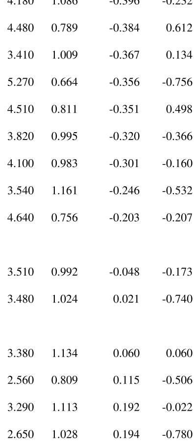
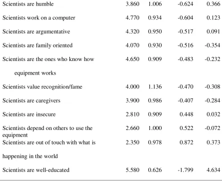
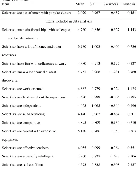
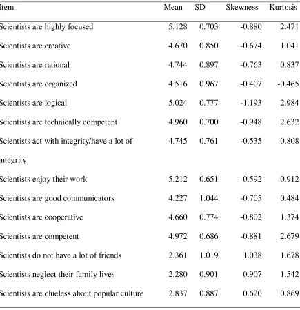
In order to answer research question 1, which asked what stereotypes chemistry students held at Time 1, skewness and kurtosis statistics were analyzed for the pre-test data on the Observations of Scientists scale. Since the focus of this project is on stereotypes, which are commonly shared perceptions of scientists, normally distributed items are not included in the data analysis. Sixteen items were removed because skewness was lower than .40, ten items were removed because kurtosis was lower than .40, and one item was removed because kurtosis was higher than 4.0 (Table 1).
Table 1
Items on Stereotypes of Scientists Scale
Item Mean SD Skewness Kurtosis
Items excluded from analysis because skewness was lower than .40
Scientists are effective leaders 4.180 1.086 -0.396 -0.232
Scientists are honest 4.480 0.789 -0.384 0.612
Scientists know a lot about popular culture 3.410 1.009 -0.367 0.134 Scientists design experiments 5.270 0.664 -0.356 -0.756
Scientists are collaborative 4.510 0.811 -0.351 0.498
Scientists are active socially 3.820 0.995 -0.320 -0.366
Scientists work obsessively 4.100 0.983 -0.301 -0.160
Scientists work regular hours 3.540 1.161 -0.246 -0.532 Scientists are able to learn to use new
equipment quickly
4.640 0.756 -0.203 -0.207
Scientists are emotional 3.510 0.992 -0.048 -0.173
Scientists depend on others to keep the equipment repaired
3.480 1.024 0.021 -0.740
Scientists are hip or cool 3.380 1.134 0.060 0.060
Scientists are absent minded 2.560 0.809 0.115 -0.506
Scientists are money oriented 3.290 1.113 0.192 -0.022
Table 1 Continued
Item Mean SD Skewness Kurtosis
Scientists are the ones who fix equipment that is broken
3.400 1.111 0.302 -0.455
Items excluded from data analysis because kurtosis was lower than .40 or higher than 4.0
Scientists are humble 3.860 1.006 -0.624 0.366
Scientists work on a computer 4.770 0.934 -0.604 0.123
Scientists are argumentative 4.320 0.950 -0.517 0.091
Scientists are family oriented 4.070 0.930 -0.516 -0.354 Scientists are the ones who know how
equipment works
4.650 0.909 -0.483 -0.232
Scientists value recognition/fame 4.000 1.136 -0.470 -0.308
Scientists are caregivers 3.900 0.986 -0.407 -0.284
Scientists are insecure 2.810 0.909 0.448 0.032
Scientists depend on others to use the equipment
2.660 1.000 0.522 -0.072 Scientists are out of touch with what is
happening in the world
2.350 0.978 0.872 0.373
Scientists are well-educated 5.580 0.626 -1.799 4.634
Items excluded because of correlation with partner item
Table 1 Continued
Item Mean SD Skewness Kurtosis
Scientists are out of touch with popular culture 3.020 0.967 0.457 0.454 Items included in data analysis
Scientists maintain friendships with colleagues in other departments
4.760 0.856 -0.927 1.443
Scientists have a lot of money and other resources
3.980 1.008 -0.400 0.786
Scientists have fun with colleagues at work 4.380 0.913 -0.692 0.527 Scientists know a lot about the latest
discoveries
4.751 0.968 -1.281 2.980
Scientists are work-oriented 4.882 0.779 -0.724 1.125
Scientists teach others about the equipment 4.480 0.799 -0.704 0.995
Scientists are independent 4.653 1.065 -0.966 0.996
Scientists are self-sacrificing 4.140 0.962 -0.664 0.601
Scientists are competitive 4.895 0.809 -0.634 0.710
Scientists are careful with expensive equipment
5.140 0.786 -1.156 2.763
Scientists are effective teachers 4.055 0.999 -0.764 0.551 Scientists are especially intelligent 4.900 0.827 -1.035 3.106
Table 1 Continued
Item Mean SD Skewness Kurtosis
Scientists are highly focused 5.128 0.703 -0.880 2.471
Scientists are creative 4.670 0.850 -0.674 1.041
Scientists are rational 4.744 0.897 -0.763 0.837
Scientists are organized 4.516 0.967 -0.407 -0.465
Scientists are logical 5.024 0.777 -1.193 2.984
Scientists are technically competent 4.960 0.700 -0.948 2.632 Scientists act with integrity/have a lot of
integrity
4.745 0.761 -0.535 0.808
Scientists enjoy their work 5.212 0.651 -0.592 0.912
Scientists are good communicators 4.227 1.044 -0.705 0.484
Scientists are cooperative 4.660 0.774 -0.802 1.374
Scientists are competent 4.972 0.686 -0.881 2.679
Scientists do not have a lot of friends 2.361 1.019 1.038 1.678 Scientists neglect their family lives 2.280 0.901 0.907 1.542 Scientists are clueless about popular culture 2.837 0.887 0.620 0.869
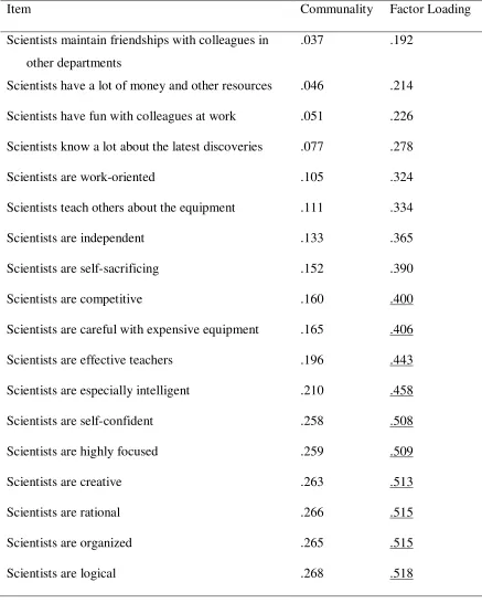
scree plot was generated using Principal Axis Factoring and based on the scree plot, it was determined that there were three viable factors.
A second EFA was then conducted, in which a forced three-factor solution was obtained using Principal Axis Factoring and a Promax Rotation. A factor loading of .40 or above indicated that an item loaded on a given factor. Items that had factor loadings of .399 or below were dropped. Items with comparable factor loadings on both factors were also dropped. In the three-factor solution, two of the factors had a high level of
correlation (R=.526) and as a result, multiple items loaded on both factors. Cronbach’s alphas for each factor on the three factor solution were also low (Factor 1: α = .673; Factor 2: α = .726; Factor 3: α = .484). Therefore, it was determined that a three factor solution was not viable for this scale.
A two-factor solution was then considered, but it was noted that all the items that had been negatively worded on the initial scale loaded on one factor. Since this is a documented problem with negatively worded questions (Spector, Van Katwyk, Brannick, & Chen, 1997), the following negatively worded items were removed from the analysis: “Scientists do not have a lot of friends,” “Scientists neglect their family life,” and
Table 2
Exploratory Factor Analysis Results for Observations of Scientists Scale, Time 1
Item Communality Factor Loading
Scientists maintain friendships with colleagues in other departments
.037 .192
Scientists have a lot of money and other resources .046 .214 Scientists have fun with colleagues at work .051 .226 Scientists know a lot about the latest discoveries .077 .278
Scientists are work-oriented .105 .324
Scientists teach others about the equipment .111 .334
Scientists are independent .133 .365
Scientists are self-sacrificing .152 .390
Scientists are competitive .160 .400
Scientists are careful with expensive equipment .165 .406
Scientists are effective teachers .196 .443
Scientists are especially intelligent .210 .458
Scientists are self-confident .258 .508
Scientists are highly focused .259 .509
Scientists are creative .263 .513
Scientists are rational .266 .515
Scientists are organized .265 .515
Table 2 Continued
Item Communality Factor Loading
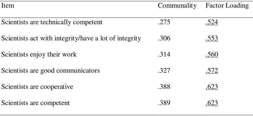
Scientists are technically competent .275 .524
Scientists act with integrity/have a lot of integrity .306 .553
Scientists enjoy their work .314 .560
Scientists are good communicators .327 .572
Scientists are cooperative .388 .623
Scientists are competent .389 .623
To test the second hypothesis, which stated that there will be a change in the mean factor score for the intervention group from Time 1 to Time 2, mean scores were
computed for each participant for their observations of scientists. A repeated measures ANOVA was conducted in order to determine the interaction of time (pre/post test) and group membership (intervention or control) on the mean factor scores. This analysis indicated that time was a significant predictor of the mean factor score (F (1) = 5.21, p = .02), but neither group membership (F (1) = 1.56, p = .21) nor the interaction between group membership and time (F (1) = .336, p = .56) predicted mean factor scores. Thus, there was a significant change in the mean factor scores from Time 1 to Time 2 for the full sample, but this change was not dependent on group membership.
in the mean factor scores of the control group and the intervention group on the Observations of Scientists scale at Time 1 and Time 2. This test revealed that in the control group, there were no significant changes in the mean factor score from Time 1 to Time 2, t(25) = 1.46, p = .16, η2 = .15. This indicates that there was no significant difference in the stereotypes of the control group from the pre- to the post-test.
In the intervention group, the t-test revealed that there was a significant difference between the mean factor scores at Time 1 and Time 2, t(89) = 2.79, p = .007, η2 = .14. There was a decrease in the mean factor scores from Time 1 to Time 2, indicating that participants were agreeing less strongly with stereotypes at Time 2 than at Time 1.
Fit Score
To test hypotheses 3-6, a difference score was created by subtracting each participant’s responses on the Observations of Scientists scale from his or her
Group Differences in Fit
In order to test hypothesis 3, which posited that the fit score would be similar for students in the intervention and control groups at Time 1, an independent samples t-test was conducted on the fit score at Time 1 comparing the mean fit scores of the
intervention group with the mean fit scores of the control group. This analysis returned non-significant results, t(112) = .08, p = .94, η2 = .01. This indicates that there was no difference in fit score at Time 1 between the intervention and control groups.
To test hypothesis 4, which posited that the intervention group would have significantly lower fit scores than the control group at Time 2, another independent samples t-test was conducted using Time 2 scores, with the fit score as the dependent variable and group membership as the independent variable. This test also returned non-significant results, t(111) = -.07, p = .94, η2 = .01. This indicates that after the
intervention, at Time 2, there was still no significant difference in fit score between the intervention and control groups.
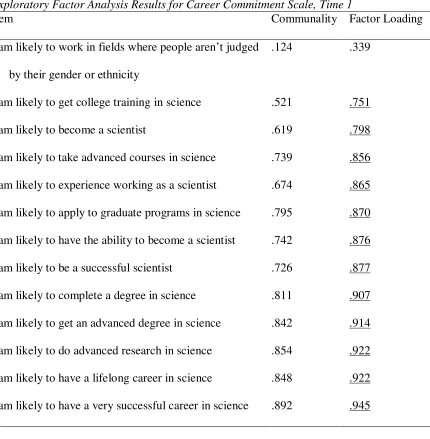
Fit and Career Commitment
The resulting analysis revealed one viable factor, which explained 73.62% of the variance on the scale and had a Cronbach’s alpha of .975.
Table 3
Exploratory Factor Analysis Results for Career Commitment Scale, Time 1
Item Communality Factor Loading
I am likely to work in fields where people aren’t judged by their gender or ethnicity
.124 .339
I am likely to get college training in science .521 .751
I am likely to become a scientist .619 .798
A mean score was then created for each participant on the resulting factor on the scale by summing the scores on each item and dividing by the total number of items in that factor to represent a range from low to high commitment on a scale of 1 to 6. At Time 1, the mean of this career commitment score for the full sample was 4.15, the standard deviation was 1.42, skewness was -.72, and kurtosis was -.69.
Since the Fit score was significantly positively skewed, a log transformation was conducted. Next, a Pearson’s correlation was conducted with the career commitment score as the dependent variable and the transformed fit score as the independent variable. The Pearson’s correlation was non-significant, r = -.14, p = .07, indicating that there is no significant relationship between the fit score and career commitment.
Effects of Gender
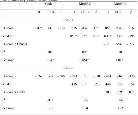
Next, a repeated measures 2x2 Analysis of Variance was conducted on the
intervention group to test the effects of gender on the relationship between time (pre/post test) and fit score (Table 4). This test had no significant results, revealing that neither time nor gender was a significant predictor of fit score and that there was no significant interaction between gender and time in predicting fit score. When the results were analyzed graphically, it appeared that men had a better fit between stereotypes of
Figure 1. Fit Scores by Time and Gender
Another set of ANOVAs was conducted to determine whether gender impacted the relationship between group membership (intervention/control) and fit score (Table 4). These tests revealed that the fit score was not significantly different across group or gender and furthermore, that there was no significant interaction between group and gender to determine fit score at either Time 1 or Time 2. Thus, gender did not influence the relationship between group membership and fit score at either time.
Table 4
Analysis of Variance Results, Gender
F Df p η2
Interaction of time and gender on fit score
Time .008 1 .931 <.001
Gender 2.41 1 .123 .023
Time*Gender 1.82 1 .181 .018
Interaction of group and gender on fit score at Time 1
Group .023 1 .880 <.001
Gender 1.36 1 .246 .012
Group*Gender .478 1 .491 .004
Interaction of group and gender on fit score at Time 2
Group .022 1 .883 <.001
Gender .091 1 .763 .001
Group*Gender .757 1 .386 .007
At Time 1, gender was found to be a significant predictor of career commitment such that women had higher career commitment than men, but there was no relationship between the fit score and career commitment, nor was there an interaction between gender and fit score to predict career commitment. At Time 2, there were no significant results, indicating that neither gender nor fit score significantly predicted career
Table 5
Hierarchical Regression Results, Gender
Model 1 Model 2 Model 3
B SE B β B SE B β B SE B β
Time 1
Fit score -.475 .410 -.125 -.676 .404 -.177 .060 .834 .016
Gender .856* .327 .278* .800* .332 .259*
Fit score * Gender -.961 .954 -.217
R2 .016 .090 .101
F change 1.342 6.851* 1.015
Time 2
Fit score -.167 .379 -.049 -.241 .381 -.070 -.464 .746 -.135
Gender .436 .321 .150 .448 .325 .154
Fit score*Gender .303 .869 .075
R2 .002 .025 .026
F change .195 1.84 .122
*significant at p = .05
Exploratory Analyses
were conducted. These analyses took into consideration the additional variables of major, self image, and individual level beliefs about scientists.
Major
Since the participant pool was an introductory Chemistry course, both STEM majors and non-majors frequently enroll in the course. Thus, an exploration of the effects of major was carried out. The initial survey listed a total of 37 possible majors. In order to complete these analyses, the major variable was recoded such that all participants were broken down into STEM majors, non-STEM majors, and those who reported that they were undecided or that their major was not listed. At Time 1, there were 83 (65.9%) STEM majors, 9 (7.1%) non-STEM majors, and 34 (27%) participants who were undecided or who marked their major as “Other.” At Time 2, there were 90 (71.4%) STEM majors, 7 (5.6%) non-STEM majors, and 29 (23%) of participants who were undecided or marked their major as “Other.”
participants’ career scores (p = .90). A graphical analysis (Figure 2) revealed that STEM majors had higher career scores than non-majors or undecided participants.
Figure 2. Career Scores by Major, Time 1
STEM majors continued to have higher career scores than non-majors or undecided participants.
Figure 3. Career Scores by Major, Time 2
gender (Table 6). Graphical analyses revealed that men who were non-STEM majors had higher career scores than women who were non-STEM majors, but that women who were STEM majors had higher career scores than men who were STEM majors. At Time 1 (Figure 4), undecided participants had similar career scores, regardless of gender, but at Time 2 (Figure 5), men in the undecided group had higher career scores than did women.
0
1
2
3
4
5
6
STEM
Non STEM
Undecided/Other
Major
C
a
re
e
r
s
c
o
re
Males
Females
0
1
2
3
4
5
6
STEM
NonSTEM
Undecided/Other
Major
C
a
re
e
r
S
c
o
re
Males
Females
Figure 5. Career Score by Major and Gender, Time 2
Table 6
Analysis of Variance Results, Major
F Df p η2
Interaction of major and gender on career score at Time 1
Major 26.42 2 <.001 .313
Gender .239 1 .626 .002
Major*Gender 3.08 2 .050 .050
Interaction of major and gender on career score at Time 2
Major 11.46 2 <.001 .165
Gender .908 1 .448 .005
Major*Gender 5.38 2 .036 .056
Interaction of major and gender on fit score at Time 1
Major .689 2 .504 .124
Gender 26.4 1 <.001 .196
Major*Gender 10.9 2 <.001 .168
Interaction of major and gender on fit score at Time 2
Major .600 2 .551 .011
Gender 1.82 1 .180 .017
Figure 6. Fit Score by Major and Gender, Time 1
Self Image
A self-image score was computed for each participant, based on his or her scores on the 16 self-image items that corresponded to the 16 scientist stereotype items that remained in the analyses after the EFA. An independent samples t-test was conducted to determine whether there were any differences in this self-image score across gender and
it revealed that there were no significant differences at Time 1 (t = -.145, p = .885) or at Time 2 (t = -.107, p = .915).
Individual Level Beliefs about Scientists
The Fit score that was used in all previous analyses was computed based on group level stereotypes about scientists and the self-image items that corresponded with these group level stereotypes. However, it is possible that individual level beliefs about scientists are more important than group level stereotypes when predicting the outcomes that are of interest in this study. Therefore, a second version of the Fit score was
computed using all the scientist and self-image items. First, a difference score was obtained for each set of corresponding scientist and self-image items, then the absolute value of this score was computed. Finally, all the absolute values were added together and then divided by the total number of paired items (56). This new variable was named “Total Fit.” At Time 1, Total Fit had a mean score of .950, a standard deviation of .347, skewness of .939, and kurtosis of .474. At Time 2, M = .899, SD = .402, skewness = .696, and kurtosis = .947.
All previous analyses that used the Fit score were conducted again, using the Total Fit score. First, independent samples t-tests were conducted at Time 1 and at Time 2 to determine whether there were differences on the Total Fit based on group
control group members on the Total Fit score at Time 1 (t = -.73, p = .47) or at Time 2 (t
= -.74, p = .46).
Next, a log transformation was conducted on the Total Fit score since it was significantly positively skewed and a Pearson’s correlation was conducted on the full sample (intervention and control group) at Time 1 to determine whether there was any relationship between Total Fit score and career commitment. This test revealed that there was a significant negative correlation between Total Fit score and career commitment (r
= -.22, p = .01). This indicates that individuals with higher Total Fit scores had lower career commitment. Since higher scores on Total Fit actually indicate a worse fit
between individual beliefs about scientists and self-image, this can be interpreted to mean that individuals with better fit between individual beliefs about scientists and self-image have higher career commitment to STEM.
Table 7
Analysis of Variance Results, Total Fit Score
F Df p η2
Interaction of group and gender on total fit score at Time 1
Group .296 1 .588
Gender .458 1 .500
Group*Gender 2.76 1 .100
Interaction of group and gender on total fit score at Time 2
Group .271 1 .604
Gender 1.72 1 .193
Group*Gender .908 1 .343
Table 8
Hierarchical Regression Results, Total Fit Score
Model 1 Model 2 Model 3
B SE B β B SE B β B SE B β
Time 1
Fit score -.887* .449 -.222* -1.3* .431 -.314* -1.39 .803 -.348
Gender 1.15* .326 .381* .977 .928 .324
Fit score * Gender .187 .954 .075
R2 .049 .164 .153
F change 3.90* 12.4* .039
Time 2
Fit score -.162 .415 -.047 -.276 .436 -.080 -1.10 .872 -.319
Gender .326 .374 .110 -.601 .928 -.203
Fit score*Gender 1.10 1.01 .466
R2 .002 .013 .030
F change .152 .759 1.19
*significant at p = .05
Discussion
relatively new field of study and rarely has research been devoted to the effects of students’ stereotypes on their career commitments. Furthermore, most of the interventions that have been developed and empirically analyzed have focused on practical outcomes such as course grades and evaluation of classroom climates, rather than a broader change in students’ views of STEM fields (Bennet & Lubben, 2006; Brickhouse, Carter, and Scantlebury, 1990; Wenzel, 2001; Wight & Burn, 1991). Thus, it is unclear what stereotypes students currently hold about science and scientists.
However, according to career commitment literature, students’ views of the environment within STEM fields could be extremely important to long-term retention (Holland, 1997, Ployhart, Weekley, & Baughman, 2006). Furthermore, the extent to which they feel that their personal characteristics match their preconceptions about STEM fields could be expected to influence persistence in the face of challenges within these fields (Schaefers, Epperson, & Nauta, 1997).
The current study explored student stereotypes in one area of STEM, which is helpful in building subject-specific knowledge about stereotypes. A learning intervention that focused on introducing women’s achievements to chemistry was piloted.
Stereotypes and career commitment were measured both before and after the