Load Bearing Capacity of Degraded Nuclear Piping

(1)

18th International Conference on Structural Mechanics in Reactor Technology (SMiRT 18) Beijing, China, August 7-12, 2005 SMiRT18-G08-3

LOAD BEARING CAPACITY OF DEGRADED NUCLEAR PIPING

E. Roos, K.-H. Herter, X. Schuler

MPA, University of Stuttgart, Pfaffenwaldring 32, D-70569 Stuttgart, Germany

Phone: +49 711 685 2601, Fax: +49 711 685 3053

E-mail: xaver.schuler@mpa.uni-stuttgart.de

J. Chattopadhyay, B.K. Dutta, H.S. Kushwaha

Bhabha Atomic Research Centre (BARC), RSD, Hall-7, Mumbai – 400085, India

E-mail: jchatt@apsara.barc.ernet.in

ABSTRACT

Integrity assessment of piping components with postulated cracks is important for safe and reliable operation of power plants. While various equations and methods are available for prediction of the load bearing capacity of pipes and elbows, it is very important to choose the correct equation and method whose predictions are consistent, safe but not too conservative with respect to the experimental results. Towards this goal, a comprehensive Component Integrity Assessment Program was initiated under a joint MPA-BARC collaborative program where a large number of austenitic and ferritic pipes and elbows of nominal diameter of 50 – 400 mm with various crack configurations and sizes were tested. These test results along with results of previous tests were analysed with various available limit load equations present and also with the R6 method. Based on the comparison of these test results and predictions, the correct equation and method are recommended to reliably predict the load bearing capacity of flawed pipes and elbows reliably.

Keywords: Integrity assessment, piping, leak-before-break (LBB) behaviour, analytical/numerical and

experimental investigations, engineering and fracture mechanics methods, limit load calculations

1. INTRODUCTION

The investigation of the failure behaviour of pipes has been an evolutionary process that was initiated from the gas and oil industry to understand large breaks occurring in pipeline systems. The main work in piping systems started about 1950. Since that time numerous investigations in the experimental and numerical field were performed so that the failure behaviour and failure load of pipes could be well assessed and hence the safety margin also. With the start of operation of commercial nuclear power plants there was an additional need for tools to assess reliably the failure behaviour of piping systems under different loading and environmental conditions.

In all countries, power plants are designed, constructed and operated on the basis of safety criteria, guidelines and technical codes, for example ASME (2001). There are requirements also for nuclear power plants to take into account not only the stresses resulting from operating loads but also the impacts of accidents upon the integrity of pressurized components. Such accident considerations include extreme loads, for example, earthquake and postulated pipe failure. For these loading conditions it must be demonstrated that either catastrophic failures can be excluded or, otherwise, that resultant consequential damage will not lead to critical accident sequences. This is the object of the integrity concept. Therefore, it is very important that the analytical calculation methods for integrity assessment of degraded piping components are properly validated with respect to experimental results. Towards this goal, fracture tests have been carried out on cracked piping components made of ferritic and austenitic steel under various loading combination of internal pressure and bending moment. These test results have been further analysed by various analytical methods, e.g. plastic limit load (PLL), R6 method, etc. This paper describes the experimental procedure, test results and analysis.

(2)

There are various analytical methods, e.g. plastic limit load, R6 method, etc., to assess the integrity of piping components with cracks subjected to static loads. These methods are briefly described below.

2.1 Plastic Limit Load

For small size piping components or pipes made of very tough material, the role of fracture mechanics in assessment of integrity may not be significant. This is because the plastic zone near the crack tip engulfs the entire tensile ligament before the crack driving force exceeds the material fracture toughness. For these cases, the plastic limit load governs the load bearing capacity of the component rather than the unstable fracture load. There are various plastic limit load formulae for piping components. The plastic limit moment of a through-wall circumferentially cracked pipe subjected to bending moment is calculated as follows (Kanninen et al,1982) :

ML = 4R2 tσf [cos(θ/2) - 0.5 sin(θ)] (1)

where, R is the mean radius of the pipe cross section, t is the wall thickness, σf is the pipe material flow

stress taken as the average of yield and ultimate stress i.e. σf=0.5(σy+σu) and θ is the semi-crack angle. Kastner

et al (1981) have observed that the choice of flow stress has a great influence in the estimation of critical crack lengths (and hence the critical moments also), especially for large crack size. While using σf=(σy+σu)/2.4 for

axially cracked pipes under internal pressure, Kastner et al obtained all the experimental results conservatively with respect to the theoretical predictions. Moulin and Delliou (1996) also suggest a reduction factor of ‘0.85’ to Eq. (1) to account for crack propagation at maximum moment. This is comparable to the definition of σf=(σy+σu)/2.4 instead of σf=(σy+σu)/2 in Eq. (1). For a conservative estimate of limit load, one can set the flow

stress equal to the yield stress i.e. σf=σy in Eq. (1).

In the case of combined internal pressure and bending moment, the plastic collapse moment is given as (Kanninen et al, 1982):

ML = 4R2 tσf [2cos(α/2) - 0.5 sin(θ)] (2)

with

α = 0.5θ + (pπRi2)/(4Rtσf) (3)

where p is the internal pressure and Ri is the internal radius of the pipe.

For an elbow with a through-wall circumferential crack under in-plane bending moment, the limit moment is given by Zahoor (1990), Miller (1988) and very recently by Chattopadhyay et al (2004). Zahoor (1990) and Miller (1988) do not differentiate between closing and opening mode of bending moment. However, it is well known that deformation characteristics of elbow under these two bending modes are distinctly different. Considering this aspect, Chattopadhyay et al (2004) give separate limit moment formulae for closing and opening moments. The limit moment equation given by Zahoor (1990) is :

    

  

      −       −

      −

=

3 2

0559 1 0485

0 2137

0 1

D a . D a . D

a .

M

ML o (4)

3 / 2 2 f o 0.935 D th

M = σ (5)

The range of applicability is a/D≤0.8 , h=4Rbt/D2 ≤0.5 and D/t≥15, where, a is the half crack length, D is the

mean diameter of the elbow cross section, Rb is the mean bend radius of the elbow, t is the elbow wall thickness,

h=4Rbt/D2 is the elbow factor and σf is the material flow stress, usually taken as the average of yield and ultimate

strengths.

The limit moment equation given by Miller (1988) is as follows:

ML = Mo [ 1.0 – 1.5(θ/π)] (6)

where, Mo is as defined in Eq. (5) and θ is the semi-circumferential crack angle.

The limit moment according to Chattopadhyay et al (2004) is as follows:

Closing mode

X M

ML = 0 (7)

(3)

M0 = 1.075 h2/3 (4R2tσy) (8)

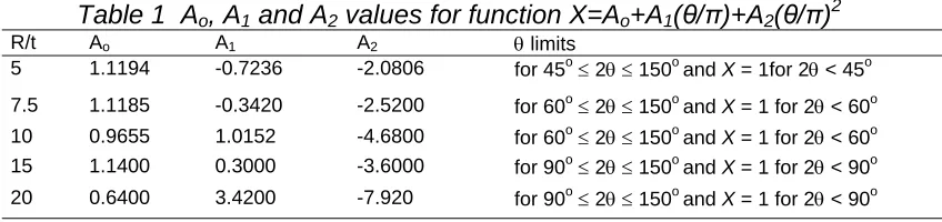
The function X is shown in Table 1.

Table 1 A

o

, A

1

and A

2

values for function X=A

o

+A

1

(

θ

/

π

)+A

2

(

θ

/

π

)

2

R/t Ao A1 A2 θ limits

5 1.1194 -0.7236 -2.0806 for 45o≤ 2θ≤ 150o and X = 1for 2θ < 45o

7.5 1.1185 -0.3420 -2.5200 for 60o≤ 2θ≤ 150o and X = 1 for 2θ < 60o

10 0.9655 1.0152 -4.6800 for 60o≤ 2θ≤ 150o and X = 1 for 2θ < 60o

Opening mode

Same form as Eq. (7) used for 5≤R/t≤ 20 with Mo and X given as follows :

M0 = (1.0485 h1/3 – 0.0617) (4R2tσy) (9)

      π θ −

=1.127 1.8108

X or 45o≤ 2θ≤ 150o (10)



     π θ −

=1 0.8 or 0o≤ 2θ≤ 45o

The limit moment for a short radius elbow (Rb/D=1) with an axial through wall crack at the crown is given by

Zahoor (1990) as follows :

   

 

      − =

D a 15 . 0 1 M

M_L _o (11)

Mo is as defined in Eq. (5). The range of applicability is: a/D≤0.9 , h=4Rbt/D2 ≤0.5 and D/t≥15

2.2 R6 Approach

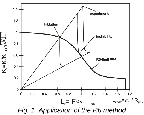
The R6-Method is based on the idea that, depending on the materials condition, failure of a component can take any form from brittle fracture to fully plastic deformation with the transition between the two extreme points being assumed to be continuous.

The limit curve was defined as follows:

Kr = (1 – 0.14 L ) (0.3 + 0.7exp.( – 0.65 L ) (12)

2 r

6 r

and

Lr(max) = σf / σy and σf = (σy + σf)/2 (13)

The loading parameters of the pipe are given by Lr=F/Fcollapse as ratio of actual load F to plastic limit load Fcollapse

and Kr=KI/KIc= J/Ji as ratio of actual stress intensity factor KI as a function of crack size and the fracture

mechanics material characteristic KIc for linear-elastic and Ji for elastic-plastic conditions (Milne et al, 1986).

In the above equation, J is derived from the linear elastic KI value. According to this concept, the onset of

stable crack extension occurs when the load point formed by Lr and Kr is on the limit curve. Instability is derived

from the load path, which forms a tangent to the limit curve, taking into consideration stable crack extension. A schematic diagram of the application of this procedure is shown in Figure 1. For this purpose, the constant load F acting in Lr is normalized by the crack-length-dependent limit load Fcollapse (a+∆a). The normalization of KI, for

example, for the applied J-integral, is carried out according to J=J(a+∆a) with the likewise crack-length-dependent KIc curve (JR (∆a)) being used as a material characteristic, taking into account also the crack extension.

However, for this procedure, it is important that piping component should have the same or less stress triaxiality (constraint) in the ligament of the cracked section compared to that of the fracture mechanics specimens.

(4)

σy

Fig. 1 Application of the R6 method

3. FRACTURE TESTS ON PIPING COMPONENTS

To validate various analytical methods for integrity assessment of degraded piping components as described above, a number of fracture tests have been carried out on pre-cracked pipes and elbows made of ferritic and austenitic steel under the comprehensive Component Integrity Test Program (Chattopadhyay et al, 2000, Chattopadhyay et al, 2005, Roos et al, 2000). These are described briefly in the following paragraphs.

3.1 Test Boundary Conditions 3.1.1 Material

The pipes of nominal diameters DN50, DN80 and DN300 were fabricated of the austenitic material X 10 CrNiNb 18 9 and those of nominal diameter DN200 from the material X 10 CrNiTi 18 9. In addition pipes and elbows of nominal diameters DN200 and DN400 were fabricated of the ferritic material SA333Gr6. The characteristic strength, ductility and fracture mechanics properties were determined as shown in Table 2. All the values are higher than the requirements given in the nuclear safety standards.

Table 2 Material properties

Pipe/ Material

Elbow

Yield Strength (0.2% proof stress)

σy (MPa)

Ultimate Tensile Strength

σu (MPa)

Young’s Modulus E (MPa)

Reduction of Area Z (%)

Elongation A5

(%)

Ji

(stretched zone) (N/mm)

DN400 SA333Gr6

Base metal 312 459 203000 70 41 236

DN300 X 10CrNiNb 18 9 Base metal Weld metal

253 442

577 635

197 000 170 500

71 52

61 37

213-361 80-117 DN200 X 10CrNiTi 18 9

Base metal Weld metal

227 467

579 695

197 800 196 600

78 48

60 35

302-398 73-146

DN200 SA333Gr6

Base metal 288 420 203000 70 36 220

DN80 X 10CrNiNb 18 9

259 619 198 500 80 58 229-258

288-317

DN50 X 10CrNiNb 18 9

260 636 191 300 78 56 229-258

288-317

3.1.2 Test Specimens and Set up

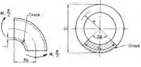
Test specimens consisted of pipes or elbows with through-wall or part-through circumferential cracks under combined internal pressure and bending moment or in some cases pure bending moment. Figures 2a and 2b show the crack configurations in the elbows. In the case of elbows, straight pipes of length 400-600 mm were welded on either side to allow free ovalisation of the elbow cross section. All the specimens were fatigue

(5)

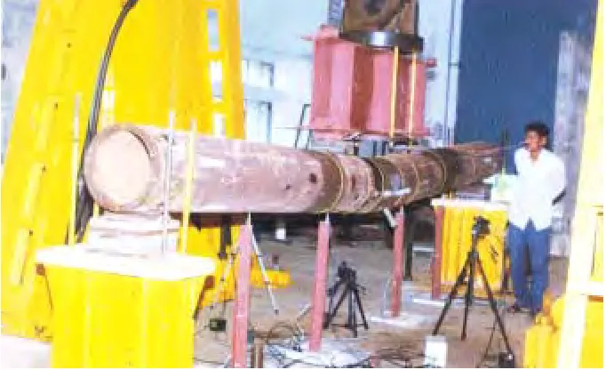
cracked by remote loading. Loading of the austenitic test pipes was achieved by internal pressure and a superimposed external bending moment using bending rigs specially made for these tests, Figure 3. The bending moment was introduced into the test pipe through a lever arm and extension pipes by means of two double acting (push-pull) hydraulic cylinders. In the case of ferritic pipes, moment loading was applied through the four point bending arrangement shown in Figure 4. In the case of elbows, the loading arrangement is shown in Figure 5. The moment loading was applied quasi-statically in all cases. Tables 3 and 4 give the details of the test specimens.

Fig. 2a. Sketch of elbow with through

wall circumferential crack at the

intrados

Fig. 2b Sketch of elbow with through

wall axial crack at the crown

3.2 Test Results 3.2.1 Austenitic pipes

Load Bearing and Deformation Behaviour

A characteristic feature for the description of the overall behavior is the applied loading plotted against the deformation (e.g. pipe bend angle). The high capacity for deformation of all pipes (with and without cracks) could be demonstrated. All the test pipes could be loaded up to the attainment of the maximum possible bend angle limited by the bending rig or beyond the maximum loading (peak load) of the test pipes without the occurrence of failure in the form of massive fracture (no unstable crack extension). The collapse load determined in accordance with ASME III. App. II-1430 was clearly exceeded in all the tests. The strain measurements showed the bending moment introduced was practically constant along the pipe axis and agreed with the moment determined from the hydraulic cylinder pressure.

Table 3 Test matrix of pipes

Pipe Dimensions Material Crack Four point

bending loading span (mm) Nominal

Diameter OD (mm)

Thickness (mm)

Depth (a/t)

Angle 2θ (o)

Internal pressure (MPa)

Outer Inner

DN400 406 32.3 SA333Gr6 1.0 96 – 158 0 5820 1480

DN300 331 32.1 X 10 CrNiNb 18 9 0.5 – 1.0 60 – 120 16 - -

DN200 219.1 14.2 X 10 CrNiTi 18 9 0.5 – 1.0 120 – 270 7 - -

DN200 219 15.1 SA333Gr6 1.0 66 – 157 0 4000 1480

DN80 88.9 8.8 X 10 CrNiNb 18 9 0.25 – 1.0 60 – 120 16 - -

DN50 60.3 8.8 X 10 CrNiNb 18 9 0.25 – 1.0 60 – 120 16 - -

As compared with the behaviour of uncracked pipes, cracks of depth up to a/t=0.75 (t wall thickness, a crack depth) and circumferential extent 2θ up to 120O (θ - half the crack circumferential angle) in the DN50 and DN80 pipes, of depth up to a/t=1.0 and circumferential extent 2θ up to 60o in the DN200 pipes and of depths up to a/t=0.5 and circumferential extent 2θ up to 120o in the DN300 pipes merely caused a small reduction in the overall load bearing capacity. Depending on the pipe and crack geometry, in the majority of the tests conducted the bending moment could be raised increasingly up to the maximum pipe bend angle so that by the end of the

(6)

tests the maximum load bearing capacity had still not been reached as is shown for example in Figures 6 to 8 for tests on pipes of DN300, DN200 and DN80 mm nominal diameter.

Fig. 3 Photograph of fracture test

set-up of austenitic pipe

Fig. 5 Photograph of fracture test

set-up of elbow

Fig. 4 Photograph of fracture test set-up of ferritic pipe under four point bending load

Failure Behaviour

(7)

Crack initiation took place each time clearly before the theoretical collapse load or before the maximum loading attained in the test. Crack initiation was determined by potential probe measurements and photographic records.

• Pipes of DN50 nominal diameter (austenitic material): In tests with defect dimensions a/t=0.25 with 2θ=120O and a/t=0.75 with 2θ=60O no crack initiation could be determined. In the remaining tests even with circumferential slits (a/t=1) only slight stable crack growth occurred.

• Pipes of DN80 nominal diameter (austenitic material): In tests with defect dimensions a/t=0.25 with 2θ=120O no crack initiation could be determined. In the remaining tests even with a circumferential through-wall crack (a/t=1) only stable crack growth occurred.

• Pipes of DN200 and DN300 nominal diameter (austenitic material): Stable crack growth occurred at times following crack initiation. At no time were indications of unstable crack propagation present.

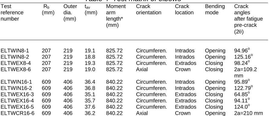
Table 4 Test matrix of elbows

Test reference number Rb (mm) Outer dia. (mm) tav (mm) Moment arm length* (mm) Crack orientation Crack location Bending mode Crack angles after fatigue pre-crack (2θ)

ELTWIN8-1 207 219 19.1 825.72 Circumferen. Intrados Opening 94.96o

ELTWEX8-4 207 219 19.3 825.72 Circumferen. Extrados Closing 98.24o

ELTWEX8-6 207 219 19.0 825.72 Axial Crown Closing 2a=109.2

mm

ELTWCR16-6 609 406 36.2 840.22 Axial Crown Opening 2a=210 mm

*Moment arm length is the perpendicular distance between the loading line and mid-section of elbow center-line for conversion of load to moment

PIPE ROTATION [Degree]

p pii= 16 MPa= 16 MPa T = 20 T = 20o o _CC Mb Oper.+Upset BE ND IN G M O M E NT [ k N m ] 0 200 400 600 1000

0 4 8 12 16 20 24 28

pipe without flaw

a/t = 1,0 2θ= 60o a/t = 1,0

2θ= 120o a/t = 0,5 2θ= 60o

without internal pressure

leakage

(Mb = 827 kNm)

p pii= 16 MPa= 16 MPa T = 20 T = 20o o _CC Mb Oper.+Upset BE ND IN G M O M E NT [ k N m ] 0 200 400 600 1000

0 4 8 12 16 20 24 28

pipe without flaw

a/t = 1,0 2θ= 60o a/t = 1,0

2θ= 120o a/t = 0,5 2θ= 60o

without internal pressure

leakage

(Mb = 827 kNm)

Fig. 6 Load bearing behaviour of

austen- itic pipes with nominal diameter

DN300 (OD 331 mm, t=32 mm) and

internal pressure 16 MPa at room

temperature

B E N D IN G MOME N T [N m] 0.00E+00 2.50E+04 5.00E+04 7.50E+04 1.00E+05 1.25E+05 1.50E+05 1.75E+05 2.00E+05

0 5 10 15 20 25 30 35

Circumf. weld 2θ=180o

a/t=0,7

pipe without flaw

2θ=180o a/t=0,7 B E N D IN G MOME N T [N m] 0.00E+00 2.50E+04 5.00E+04 7.50E+04 1.00E+05 1.25E+05 1.50E+05 1.75E+05 2.00E+05

0 5 10 15 20 25 30 35

a/t=0,7

2θ=180o a/t=0,7 0.00E+00 2.50E+04 5.00E+04 7.50E+04 1.00E+05 1.25E+05 1.50E+05 1.75E+05 2.00E+05

0 5 10 15 20 25 30 35

a/t=0,7

2θ=180o a/t=0,7

Fig. 7 Load bearing behaviour of

austen- itic pipes with nominal diameter

DN200 and internal pressure 7

MPa at room temperature

(8)

BE

ND

IN

G

M

O

M

E

N

T [k

Nm

]

0 5 10 15 20 25

0 4 8 12 16 20 24 28

M_b,collaps

leakage

pipe without

law a/t=0.25 2θ=120o

leakage

a/t=1.0 2θ=60o

a/t=0.75 2θ=60o

a/t=0.65 2θ=60o

weld a/t=0.4 2θ=120o

BE

ND

IN

G

M

O

M

E

N

T [k

Nm

]

0 5 10 15 20 25

0 4 8 12 16 20 24 28

M_b,collaps

leakage

pipe without

law a/t=0.25 2θ=120o

leakage

a/t=1.0 2θ=60o

a/t=0.75 2θ=60o

a/t=0.65 2θ=60o

weld a/t=0.4 2θ=120o

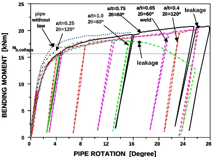
Fig. 8 Load bearing behaviour of austenitic pipes with nominal diameter DN80

In none of the tests carried out did a failure in the form of a massive fracture (large break) occur (no unstable crack propagation observed). Depending on the initial crack size and the pipe dimensions, no or only slight stable crack growth occurred (e.g. in DN50 and DN80 with defect dimensions a/t=0.25 and 2θ=120O) ranging up to pronounced stable crack growth (e.g. in DN200 and DN300 with defect dimensions equal to or greater than a/t=0.5 and 2θ=120O). In the tests in which the maximum load was attained, in all cases stable crack extension occurred up to the maximum load after crack initiation. Even after passing beyond the maximum load no unstable crack behaviour appeared. Therefore, in the tests carried out up to leakage, leak-before-break behaviour could be proven under the given loading conditions.

3.2.2 Ferritic Pipes

Pipe fracture test results are expressed in the form of load vs. load-line-displacement of the four point bending arrangement and load vs. crack growth curves. Crack growth has been measured by an image processing technique as described in (Chattopadhyay et al, 2000). Figure 9 shows the load vs. load-line-displacement curves for various pipes. The crack grows out-of-plane in the case of carbon steel pipes. The amount of crack growth is slightly different at the two crack tips. To construct the load vs. crack growth curves and generate the component J-R curves, the average projected crack growth in the plane of the initial crack is taken. Figure 10 shows the load vs. crack growth curves for various pipes.

0 50 100 150 200 250

0 200 400 600 800

DN200, 2θ = 126o DN200, 2θ = 94o

DN200, 2θ = 66o DN400, 2θ = 158o

DN400, 2θ = 126o DN400, 2θ = 96o

Load (kN)

Load line displacement (mm)

Fig. 9 Load vs. load-line-displacement

curves for various through wall

cracked ferritic pipes

0 20 40 60 80

0 200 400 600 800

DN200, 2θ = 126o DN200, 2θ = 94o DN200, 2θ = 66o DN400, 2θ = 158o

DN400, 2θ = 126o DN400, 2θ = 96o

Load (kN)

Average projected crack extension (mm)

Fig. 10 Load vs. crack growth curves

for various through wall cracked ferritic

pipes

(9)

3.2.3 Ferritic Elbows

Figures 11 and 12 show the load vs. load-line-displacement curves for 200 and 400 mm nominal diameter elbow specimens. The figure also shows the limit loads calculated by the ASME recommended twice elastic slope method. It may be noted from Figures 11 and 12 that elbows under closing moment reached the maximum load and then the load drops after the peak value indicating instability of the structure. However, elbows under opening moment reached the maximum load asymptotically without showing any drooping behavior. This is compatible with the observations of Kussmaul et al (1995).

The crack grows out-of-plane in the case of carbon steel elbows also. The amount of crack growth is slightly different at the two crack tips. To construct the load vs. crack growth curves, the average projected crack growth in the plane of the initial crack is considered. It may be noted that crack growth, observed by the image processing technique, is on the outer surface. To get the mean value, crack growth on the outer surface has been multiplied by (R/Ro). This assumes that the crack front is radial across the thickness of the elbow. No crack

growth has been observed during fracture tests of axially cracked elbows. Figures 13 and 14 show the photograph of crack growth at the end of experiment of two elbows.

0 30 60 90 120 150

0 40 80 120 160

ELTWIN8-1 (2θ = 94.960

, Opening)

ELTWIN8-2 (2θ = 125.160

, Opening)

ELTWEX8-4 (2θ = 98.240

, Closing) ELTWCR8-6 (2a = 109.2 mm, Closing) TES collapse load

Lo

ad (k

N)

Total load-line-displacement (mm)

Fig.11 Experimental load-deflection

curves from 200 mm NB elbows

0 40 80 120 160 200

0 300 600 900 1200 1500

ELTWIN16-1 (2θ = 95.89o, Opening) ELTWIN16-2 (2θ = 122.79o

, Opening) ELTWEX16-3 (2θ = 64.85o, Closing) ELTWEX16-4 (2θ = 94.11o

, Closing) ELTWEX16-5 (2θ = 124o, Closing) ELTWCR16-6 (2a = 210 mm, Opening) TES Collapse load

Loa

d (k

N)

Load line displacement (mm)

Fig.12 Experimental load-deflection

curves from 400 mm nominal diameter

elbows

Fig.13 Crack growth at end of test of

DN400 mm elbow ELTWEX16-5

(2

θ

=124

o

,Closing moment)

20

Fatigue pre-crack

Fig.14 Crack growth at the end of

experi- ment of DN200 mm through wall

axially cracked elbow (Test no.

ELTWCR8-6, 2a=109 mm,

closing moment). No crack growth was

observed.

Fatigue

pre-crack Stable crack

(10)

4. COMPARISON OF EXPERIMENTAL RESULTS WITH THEORY 4.1 Austenitic Pipes

From the tests carried out at MPA Stuttgart and accessible published data, results of tests on straight pipes (nominal diameter of 50 mm to 300 mm and wall thickness from 8 mm to 30 mm) made of austenitic materials are available. In addition the failure moments have been calculated in accordance with the PLL, with the stipulation that by suitable choice of flow stress σf the calculated failure moment should correspond with the

experimentally determined maximum moment. Figure15 shows examples for pipes of nominal diameter DN200. The good agreement of the commonly applied PLL methods with the experiments is demonstrated. To estimate the loadings (moments) at crack initiation, the R6-Method was applied to the pipe and crack geometries investigated. It turned out that independent of the pipe dimensions and crack type (surface crack or through-wall crack) the R6-Method is the most suitable for estimating the loading at crack initiation and in comparison with the test results without exception provided similar or conservative values as shown by way of example on pipes of DN200 nominal diameter in Figure 16.

0 50 100 150 200 250 300 B e n d in

g M

o m e n t M b [k N m ]

0 30 60 90 120 150 180 210 240 270

Circumferential Crack Length [Degree]

Crack depth 3.65 mm (a/t = 0.25) Crack depth 7.30 mm (a/t = 0.50) Crack depth 10.95 mm (a/t = 0.75) Crack depth 14.60 mm (a/t = 1.00) Experimental Data

D

o= 218 mm, t = 14.6 mm p_i = 7 MPa

σ_u = 582 MPa σ_y = 228 MPa σ_f = (σ_y+σ_u)/2.4 = 338 MPa

a/t=1.0 a/t=1.0 a/t=1.0 a/t=0.7 a/t=0.5 a/t=0.5 a/t=1.0 Without Crack a/t=0.7 a/t=0.7 a/t=1.0 a/t=0.4 a/t=0.7

Fig.15 Failure moments as compared

with experimental data for DN200 pipes

calculated using the plastic limit load

(PLL) concept

0 50 100 150 200 250 300 B e n d in g m o m e n t M b [k N m ]

0 30 60 90 120 150 180 210 240 270

Crack angle [degree]

Experimental initiation Experimental maximum load Limit load calcualtion by PLL Initiation by R6 Instability by R6

Outside Diameter D_o= 218 mm

Wall thickness t = 14.6 mm Crack depth a/t = 1.0

Internal pressure 7 MPa

Material: X 10 CrNiTi 18 9 σ_f = (σ_y+σ_u)/2.4 σ

y = 228 MPa σ_u = 582 MPa

Fig.16 R6-Method and limit load calcu-

lations

(

σ

f

= [

σ

y

+

σ

u

]/2.4) for pipes

with

DN200

4.2 Ferritic Pipes

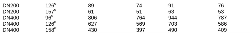
In this section, limit load analyses of fracture test results of through-wall circumferentially cracked ferritic pipes are performed. The limit loads are calculated using Eqs. (1 to 3) as described in Section 2.1. Table 5 shows the comparison of the experimentally observed maximum moment with the predictions of limit moments as per Eq. (1), with σf=σy, σf=(σy+σu)/2 and σf=(σy+σu)/2.4 . It may be seen that use of σf=σy and σf=(σy+σu)/2.4 gave

conservative results for all cases. Use of flow stress as the average of yield and ultimate stress gave quite close matching with the DN200 mm pipes. However, it gave non-conservative results in the case of DN400 mm pipes. This is because the DN200 mm pipes failed mostly in plastic collapse without much crack growth (<8 mm) until the maximum load is attained, whereas the DN400 mm pipes had stable crack growth in the range of 15 – 21 mm before the attainment of maximum load. Figure 17 shows the comparison of experimental maximum moments with the predictions as per Eq. (1) with σf=σy.

Table 5 Comparison of maximum experimental moments with theoretical predictions

Test

specification

Initial crack angle (2θ)

Experimental max. moment (kN-m)

Predicted moments using Eq.(1) (kN-m)

σf = σy σf = 0.5(σy + σu) σf = (σy + σu)/2.4

DN200 66o 155 125 153 128

DN200 94o 124 100 123 102

(11)

DN200 126o 89 74 91 76

DN200 157o 61 51 63 53

DN400 96o 806 764 944 787

DN400 126o 627 569 703 586

DN400 158o 430 397 490 409

4.3 Ferritic Elbows

The experimentally observed twice elastic slope collapse moments are compared with the theoretical predictions by Chattopadhyay et al (2004) through Eqs. (7-10), Miller (1988) through Eqs. (5,6) and Zahoor (1990) through Eqs. (4, 5 and 11). The weakening factors (ML/M0) for closing bending using the Eqs. (7 and 8)

proposed by Chattopadhyay et al (2004) for intermediate R/t have been linearly interpolated between two adjacent R/t values. To get the corresponding moment from the experimental load, load is multiplied by the perpendicular distance between the load line and middle of elbow axis which are shown in Table 4. Although this distance changes during loading of the elbow, the change has been found to be negligible compared to the initial distance and hence has not been accounted for in the calculation. In terms of applicability

0 30 60 90 120 150 180

0,0 0,2 0,4 0,6 0,8 1,0

Theoretical (σ_f = σ_y)

Experiment (DN 200 mm pipes) Experiment (DN 400 mm pipes)

M

o

m

e

nt /

4R

2 tσ

y

Circumferential crack angle (2θ), deg.

Fig.17 Comparison of theoret. limit moment (init. crack angle) with exp. maximum

moment

of Eqs. (4 and 5) and (11), although the limits of elbow factor (h=4Rbt/D2 ≤0.5) and crack length (a/D<0.8 or 0.9)

are satisfied, the condition of D/t≥15 is violated here. The flow stress of the material required as input in both Miller’s and Zahoor’s equations (Eq. 5) is defined as the average of yield and ultimate strength, which are shown in Table 2. Table 6 shows the comparison of theoretical and experimental moment values. It may be seen that the predictions by Miller (1988) is too conservative. The prediction of Chattopadhyay et al (2004) is quite close to the test results. The prediction of Zahoor (1990) was not consistent with respect to conservatism and not so accurate also.

5. CONCLUSIONS

Fracture tests on cracked austenitic and ferritic pipes and elbows of sizes ranging from nominal diameter 50 to 400 mm have been carried out. The test results have been analysed and compared with the theoretical predictions by plastic limit load and R6 approaches. From these analyses, it is recommended for safe assessment of pipes within the dimensions and materials covered in this study to use the plastic limit load concept using σf=(σy+σu)/2.4 and for other cases to use σf=σy. For through-wall circumferentially cracked elbows, it is

recommended to use the limit load Eqs. (7-10) recently proposed by Chattopadhyay et al (2004). It is also seen from this study that the R6 method is quite accurate in prediction of crack initiation loads.

Table 6 Comparison of experimental twice elastic slope collapse moments with

predictions (the brackets indicate the percent. difference with respect to

experimental values)

Predicted Collapse moment (kN-m)

Test no. Experimental

collapse moment (kN-m) Chattopadhyay et al (2004),

Eqs.(7-10)

Miller (1988), Eqs.(5,6)

Zahoor (1990), Eqs.(4,5,11)

ELTWIN8-1 98.4 101.1 (-2.7%)* 82.3 (16.4%) 112.8 (-14.6%)

(12)

ELTWIN8-2 80.0 76.0 (5%) 63.6 (20.5%) 92.65 (-15.8%)

ELTWEX8-4 108.7 100.2 (7.8%) 82 (24.6%) 113.2 (-4.1%)

ELTWEX8-6 117.2 - - 129.5 (-10.5%)

ELTWIN16-1 857.0 847.1 (1.2%) 807.9 (5.7%) 1109.6 (-29.5%)

ELTWIN16-2 699.1 678.8 (2.9%) 669.2 (4.3%) 971.8 (-39%)

ELTWEX16-3 1161.2 1092.3 (5.9%) 923.4 (20.5%) 1153.6 (0.7%)

ELTWEX16-4 985.6 962.1 (2.4%) 792.5 (19.6%) 1083.3 (-9.9%)

ELTWEX16-5 792.3 819.4 (-3.4%) 682.8 (13.8%) 993.1 (-25.3%)

ELTWCR16-6 > test range - - -

* % difference = [(experim. – predicted) /experim.] × 100%

REFERENCES

ASME Boiler and Pressure Vessel Code, Sec.III, (2001), American Society of Mechanical Engineers

J.Chattopadhyay, B.K.Dutta and H.S.Kushwaha, (2000), “Experimental and analytical study of three point bend specimens and through wall circumferentially cracked straight pipe”, International Journal of Pressure Vessels and Piping77, pp 455 – 471

J.Chattopadhyay, A.K.S.Tomar, B.K:Dutta and H.S.Kushwaha, (2004), “Closed-form collapse moment equations of through wall circumferentially cracked elbows subjected to in-plane bending moment”, Journal of Pressure Vessel Technology, ASME Transactions 126, pp 307 – 317

J.Chattopadhyay, T.V.Pavankumar, B.K.Dutta and H.S.Kushwaha, (2005), “Fracture experiments on throughwall cracked elbows under in-plane bending moments : Test results and theoretical/numerical analyses”,

Engineering Fracture Mechanics , (in press)

M.F.Kanninen, A.Zahoor, G.M.Wilkowski, I.Abousayed, C.Marschall, D.Broek, S.Sampath, H.Rhee and J.Ahmad, (1982), “Instability Predictions for Circumferentially Cracked Type 304 Stainless Steel Pipes Under Dynamic Loading”, EPRI-NP-2347, Vol.1 & 2, Electric Power Research Institute, Palo Alto, CA

W.Kastner, E.Rohrich, W.Schmitt and R.Steinbuch, (1981), “Critical Crack Sizes in Ductile Piping”, Int. Journal of Pressure Vessel and Piping9, pp 197 – 219

K.Kussmaul, H.K.Diem, D.Uhlmann and E.Kobes, (1995), “Pipe Bend Behaviour at Load Levels Beyond Design” Proceedings of 13th International Conference on Structural Mechanics in Reactor Technology, SMiRT. Brazil, G, pp 187-198.

A.G.Miller, (1988), “Review of Limit Loads of Structures Containing Defects”, Int. J. of Pres. Ves. and Piping 32, pp 197 – 327.

I.Milne, R.A. Ainsworth, A.R. Dowling and A.T. Stewart; "Assessment of the integrity of structures containing defects". R/H/R6 - Rev. 3, Central Electricity Generating Board, May, 1986

D.Moulin and P.Delliou, (1996), “French Experimental Studies of Circumferentially Through-Wall Cracked Austenitic Pipes under Static Bending”, Int. J. of Pressure Vessel and Piping65, pp 343 - 352

E.Roos, K.-H.Herter and F.Ottremba, (2000), “Testing of Pressure Vessels, Piping and Tubing”, ASM Handbook, Vol.8, Mechanical Testing and Evaluation, Oct., pp 873 - 885

A.Zahoor, (1990), Ductile Fracture Handbook, Vol.3