ABSTRACT
GRIMES, HARTLEY RAY. The Longitudinal Shear Behavior of Carbon Fiber Grid Reinforced Concrete Toppings. (Under the direction of Dr. Rudolf Seracino.)
Precast double-tee (DT) floor systems with cast-in-place concrete toppings reinforced with welded wire fabric (WWF) often suffer from durability problems along the longitudinal joints of adjacent DTs. The high strain demand along these joints leads to cracking of the concrete topping, exposing the steel reinforcement to an aggressive environment resulting in corrosion. Carbon fiber grid (G-Grid) reinforcement is proposed as a replacement for the WWF to address this problem.
This thesis presents an experimental program designed to investigate the longitudinal shear behavior of C-Grid reinforced concrete. Twenty-two single-shear test specimens were designed to simulate the joint of adjacent DTs with topping. The objective was to obtain the fundamental shear-slip behavior and compare it to that of WWF reinforced specimens. Parameters included the reinforcement ratio and grid orientation. In addition, this thesis also looks at, through direct tension tests, C-Grid’s potential to interfere with the bond between the DT and the topping. It was found that, at least in the small-scale tests, steps should be taken to prevent this premature cold joint debonding. Two methods – chairing the C-Grid, or significantly roughening the DT surface – were shown to be adequate to prevent this phenomenon.
The Longitudinal Shear Behavior of Carbon Fiber Grid Reinforced
Concrete Toppings
by
Hartley Ray Grimes
A thesis submitted to the Graduate Faculty of North Carolina State University
In partial fulfillment of the Requirements for the Degree of
Master of Science
Civil Engineering
Raleigh, North Carolina 2009
APPROVED BY:
______________________________ ______________________________
Dr. Sami Rizkalla Dr. Emmett Sumner
______________________________ Dr. Rudolf Seracino
DEDICATION
BIOGRAPHY
ACKNOWLEDGEMENTS
Firstly, the author wishes to express his thanks to Dr. Rudolf Seracino, his advisor, committee chair, and mentor for the last two and half years as well as the primary investigator for this research. Dr. Seracino’s supervision, guidance, and wisdom made this research a fulfilling and rewarding experience for the author. In addition, the author would like to extend his gratitude to the rest of his committee, Dr. Sami Rizkalla and Dr. Emmett Sumner, for their assistance in guiding this research to its completion. The author feels very fortunate to have worked with such a knowledgeable and affable committee.
The author would like to thank the Research and Development Committee of the Precast Concrete Institute for generously providing funding for this research through the Daniel P. Jenny Fellowship. For supplying essential financial, material, and technical support the author is particularly thankful to John Carson and Andrew Broadway of Chomarat and Harry Gleich of Metromont. In addition, the author would like to extend his appreciation to Greg Blaszak of BG International for his input and direction.
The author would also like to recognize the efforts of the Constructed Facilities Lab staff, including Jerry Atkinson, William Dunleavy, and Greg Lucier who were instrumental in instructing and assisting the author with the use, setup, and procedures for the various lab equipment, machinery, and electronics used to conduct the research. In addition, the author extends his gratitude to Diana Lotito, Renee Howard, and Amy Yonai for their help with administrative matters and procedures.
Special thanks are due to graduate students Barney Frankl, Vivek Hariharan, Dillon Lunn, Adolfo Obregon-Salinas, Maggie Williams, and John Wylie for their advice and support over the course of his graduate studies.
TABLE OF CONTENTS
LIST OF TABLES ...viii
LIST OF FIGURES ...ix
CHAPTER 1 INTRODUCTION ...1
1.1 GENERAL INFORMATION ...1
1.2 OBJECTIVE ...3
1.3 SCOPE...4
CHAPTER 2 LITERATURE REVIEW...5
2.1 INTRODUCTION...5
2.2 SHRINKAGE CRACKING...5
2.3 BOND STRENGTH OF TWO CONCRETE LAYERS ...6
2.3.1 Surface Roughness...6
2.3.2 Moisture Level of the Existing Concrete Surface ... 10
2.3.3 Methods of Testing Bond Strength... 11
2.4 TESTING LONGITUDIONAL SHEAR STRENGTH ... 13
2.5 SHEAR-FRICTION MODELS... 15
2.5.1 ACI 318-08... 15
2.5.2 6th Edition of the PCI Design Handbook ... 17
2.5.3 Mattock et al ... 18
2.5.4 Oehlers & Bradford... 24
CHAPTER 3 EFFECT OF C-GRID ON THE COLD JOINT BOND... 29
3.1 INTRODUCTION... 29
3.2 MATERIALS AND METHODS ... 29
3.2.1 Casting of Slabs ... 29
3.2.2 Coring of Specimens... 37
3.2.3 Experimental Procedure ... 40
3.3 RESULTS ... 44
3.3.1 C-Grid Floating... 44
3.3.2 Direct Tension Tests ... 47
3.4 DISCUSSION ... 52
3.4.1 C-Grid Float... 52
3.4.2 Direct Tension Tests ... 54
CHAPTER 4 LONGITUDINAL SHEAR-SLIP BEHAVIOR OF C-GRID REINFORCED CONCRETE ... 56
4.1 INTRODUCTION... 56
4.2 MATERIALS AND METHODS ... 56
4.2.1 Specimens... 56
4.2.2 Experimental Procedure ... 61
4.4 DISCUSSION ... 72
4.4.1 General Observations ... 72
4.4.2 C-Grid Orientation ... 72
4.4.3 Premature Debonding of the Cold Joint (Interface)... 73
4.4.4 Shear-Friction ... 75
CHAPTER 5 FURTHER STUDY OF LONGITUDIONAL SHEAR-SLIP BEHAVIOR OF C-GRID REINFORCED CONCRETE ... 77
5.1 INTRODUCTION... 77
5.2 MATERIALS AND METHODS ... 77
5.2.1 Specimens... 77
5.2.2 Experimental Procedure ... 84
5.3 RESULTS ... 84
5.4 DISCUSSION ... 94
5.4.1 Cold Joint Bond Integrity... 94
5.4.2 Comparison with WWF Reinforcement... 96
5.4.3 Other Observations ... 97
CHAPTER 6 MODELING C-GRID REINFORCED CONCRETE SHEAR CAPACITY ... 99
6.1 OVERVIEW ... 99
6.2 LONGITUDINAL SHEAR-FRICTION MODELS... 102
6.2.1 ACI 318-08... 102
6.2.2 6th Edition of the PCI Design Handbook ... 103
6.2.3 Oehlers & Bradford (Modified Mattock Model) ... 105
6.3 COMPARISON OF SHEAR-FRICTION MODELS TO EXPERIMENTAL DATA... 109
6.3.1 General ... 109
6.3.2 Comparison of ACI 318-08 to Experimental Data ... 113
6.3.3 Comparison of 6th Edition of PCI Design Handbook to Experimental Data... 115
6.3.4 Comparison of Oehlers & Bradford to Experimental Data... 117
6.4 DISCUSSION ... 123
CHAPTER 7 CONCLUSIONS ... 125
7.1 OVERVIEW ... 125
7.2 FURTHER RESEARCH ... 127
REFERENCES ... 128
APPENDICES ... 130
Appendix A : C-Grid Float Raw Data... 131
Appendix B : Tension Test Raw Data... 133
Appendix C : Concrete Compressive Strength ... 134
Appendix D : Carbon Fiber Grid Tensile Strength ... 137
Appendix F : Calculation of Difference between Measured and Predicted Shear
LIST OF TABLES
Table 2-1 CSP preparation methods ... 8
Table 2-2 Adaptation of the Mattock model to different circumstances ... 25
Table 3-1 C-Grid dimensional properties... 31
Table 3-2 Schedule of cores ... 39
Table 3-3 Float results summary ... 45
Table 3-4 Tension test summary... 48
Table 3-5 Failure plane profiles... 52
Table 4-1 Shear specimen schedule ... 58
Table 4-2 Single shear test results ... 66
Table 4-3 C-Grid strand loading conditions vs. resistance mode ... 73
Table 5-1 Shear specimen schedule (second series) ... 80
Table 5-2 WWF dimensional properties ... 80
Table 5-3 Shear test results (second series)... 86
Table 6-1 Summary of experimental data ... 101
Table 6-2 Constants c1 and c2... 107
Table 6-3 Summary of conservativeness of the shear-friction models ... 112
Table A-1 C-Grid float ... 131
Table B-1 Tension test data ... 133
Table C-1 Concrete compressive strength... 136
Table D-1 C-Grid strengths ... 140
Table E-1 WWF strengths ... 145
Table F-1 Calculated shear capacities... 147
LIST OF FIGURES
Figure 1-1 Precast DT system and longitudinal shear ... 2
Figure 1-2 Typical C-Grid and WWF ... 3
Figure 2-1 CSP tablets... 8
Figure 2-2 Methods for testing bond strength (Hindo 1990) ... 12
Figure 2-3 Single-shear test specimens diagram (Mattock & Hawkins 1972)... 14
Figure 2-4 Comparison of shear-transfer strength (Mattock & Hawkins 1972) ... 20
Figure 2-5 Effect of concrete strength on shear-transfer (Mattock & Hawkins 1972) ... 21
Figure 2-6 Corbel type push off specimen (Mattock et al 1975)... 22
Figure 2-7 Altered model (Mattock et al 1975)... 23
Figure 2-8 Modified Mattock model (Oehlers & Bradford 1995)... 27
Figure 3-1 C-Grid sizes ... 32
Figure 3-2 Restraining methods... 33
Figure 3-3 Close-up of FC and RC chairs ... 34
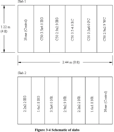
Figure 3-4 Schematic of slabs... 35
Figure 3-5 Slabs prior to casting of top layer ... 36
Figure 3-6 Marking and coring of slabs ... 38
Figure 3-7 Measuring C-Grid float in cores ... 40
Figure 3-8 Steel attachments ... 41
Figure 3-9 Jig for curing of epoxy ... 42
Figure 3-10 Epoxy curing of specimens ... 42
Figure 3-11 Schematic of specimen... 43
Figure 3-12 Specimen in MTS machine ... 44
Figure 3-13 C-Grid location after casting ... 46
Figure 3-14 Average tensile stress as a function of C-Grid size and restraint ... 49
Figure 3-15 Average tensile stress as a function of the final C-Grid location ... 50
Figure 3-16 Typical core failure planes ... 51
Figure 4-1 Shear specimen diagram... 59
Figure 4-2 Rectangular C-Grid orientations ... 60
Figure 4-3 Square C-Grid orientations... 60
Figure 4-4 Shear specimen rig ... 62
Figure 4-5 Shear specimen instrumentation and final test setup ... 62
Figure 4-6 Shear specimen failure modes ... 65
Figure 4-7 2.9x2.9 C-Grids with varying orientation ... 67
Figure 4-8 3.5x4.0 C-Grids with varying orientation ... 68
Figure 4-9 Diagonally oriented C-Grids with varying size ... 69
Figure 4-10 Perpendicularly oriented C-Grids with varying size... 70
Figure 4-11 Control specimens with compatibility comparison... 71
Figure 5-1 Surface roughness (of bottom layer of concrete)... 81
Figure 5-2 C-Grid placement methods... 82
Figure 5-3 WWF sizes (WC-CSP-4) ... 83
Figure 5-4 C150 2.4 C-Grid ... 83
Figure 5-5 Specimen B18 pre-peak load cracking... 85
Figure 5-6 Typical failure with no visible cracking (B20)... 85
Figure 5-7 Control Specimens (Second Series)... 88
Figure 5-8 WWF reinforced specimens ... 89
Figure 5-9 Comparison of WWF and C-Grid specimens (second series)... 90
Figure 5-10 Chaired C-Grid on a smooth surface finish (FC-CSP-4) ... 91
Figure 5-11 C-Grids laid flat on a rough surface finish (NR-CSP-8)... 92
Figure 5-12 Comparison of 1.6x1.8 strong oriented C-Grid from both test series... 93
Figure 5-13 Rough surface finish profile view... 95
Figure 6-1 Experimental data ... 111
Figure 6-2 Comparison of ACI 318-08 shear-friction model... 114
Figure 6-3 Comparison of PCI 6th ed. design handbook shear-friction model... 116
Figure 6-4 Comparison of Oehlers & Bradford mean shear-friction model (first series) ... 119
Figure 6-5 Comparison of Oehlers & Bradford mean shear-friction model (second series) ... 120
Figure 6-6 Comparison of Oehlers & Bradford design shear-friction model ... 121
Figure 6-7 Comparison of Oehlers & Bradford simplified design shear-friction model... 122
Figure C-1 Testing of compressive cylinders... 135
Figure D-1 Preparation of C-Grid coupons ... 139
Figure D-2 Testing of C-Grid coupons ... 139
Figure E-1 Testing of WWF coupons ... 143
CHAPTER 1 INTRODUCTION
1.1 GENERAL INFORMATION
In a typical Precast/Prestressed Double Tee (Precast DT) deck system a cast-in-place concrete topping, typically 50 to 75 mm (2 to 3 in) in thickness, is often cast on site. Amongst other things, this topping makes the entire system more rigid, especially at the longitudinal joints between two Precast DT elements. This cast-in-place topping is typically reinforced with some quantity of Welded Wire Fabric (WWF), which is simply a matrix of regularly spaced longitudinal and transverse steel wire welded together. This reinforcement is responsible for crack control of the cast-in-place topping as well as aiding in the shear transfer between the precast elements.
Figure 1-1 Precast DT system and longitudinal shear
1.2 OBJECTIVE
The main objective of this research was to determine if Carbon Fiber Grid is a suitable replacement of WWF as reinforcement of cast-in-place toppings of Precast DT systems. Currently, Carbon Fiber Grid is a proprietary material with the commercial name “C-Grid” which is produced by Chomarat North America headquartered in Anderson, SC and it is manufactured in France as well. C-Grid is a material composed of regularly spaced longitudinal and transverse strands of Carbon Fibers held together by an epoxy resin. See Figure 1-2 for a visual comparison of C-Grid to WWF.
(a) C-Grid (b) WWF
Figure 1-2 Typical C-Grid and WWF
Since Carbon Fibers are not vulnerable to corrosion like WWF, C-Grid’s suitability as a substitution for WWF as reinforcement in cast-in-place toppings will be determined by its performance related to four factors: the first two being issues unique to C-Grid, and the last two being comparisons of C-Grid to WWF.
with the cold joint bond formed between the top of the flange of the Precast DT and the cast-in-place topping (premature debonding). If premature debonding is an issue then solutions can be devised in order to avoid it. The third factor is if the shear-slip behavior of a C-Grid reinforced concrete topping is similar to that of a WWF reinforced concrete topping. The fourth and final factor is if the longitudinal shear capacity of the C-Grid reinforced toppings can be predicted using shear-friction models originally intended for use with steel reinforcement.
1.3 SCOPE
CHAPTER 2 LITERATURE REVIEW
2.1 INTRODUCTION
This Chapter presents a review of the literature relevant to the experimental program and analytical work of this research. First, a review of Carbon Fiber Grid’s (C-Grid) ability to mitigate shrinkage cracking is presented, as this is one of the reasons for adding reinforcement to cast-in-place toppings.
In addition, factors that affect the bond strength of two concrete layers are discussed. It is important to maintain the bond integrity between the cast-in-place topping and the precast deck/flange; otherwise, the structural performance will be compromised. Issues affecting bond strength include surface roughness of the existing concrete layer, which is the Precast/Prestressed Double Tee (Precast DT) within the scope of this research, and the moisture condition of said layer. Also discussed are the various methods available to test the bond strength and deciding which is best suited for the objectives and scope of this research.
Lastly, a survey of the literature is conducted reviewing various methods used to test the longitudinal shear of steel reinforced concrete as well as the development of shear-friction (or shear-transfer) models. These methods and models will be adapted to use with C-Grid reinforcement in order to compare its performance with that of Welded Wire Fabric (WWF).
2.2 SHRINKAGE CRACKING
Crack control is one of the main reasons why reinforcement is added to cast-in-place concrete toppings of precast systems. Shrinkage can be detrimental to a concrete topping as the precast element it is cast on is not shrinking, resulting in differential contraction producing internal stresses. The stresses can be enough to cause cracking in thin toppings or cause large deflections and stresses in the reinforcement (Stuart 2006). Based on this research, C-Grid has been shown to be a suitable material to control shrinkage cracking and therefore C-Grid’s ability to resist longitudinal shear needs to be determined.
2.3 BOND STRENGTH OF TWO CONCRETE LAYERS
The scope of this research involves simulating a precast Double Tee flange deck with a cast-in-place topping. This process involves casting a fresh layer of concrete (the topping) on top of another layer of concrete that has already hardened and cured (the Precast DT flange), resulting in a cold joint bond at the interface of the two layers of concrete. The strength of this bond is critical; premature debonding of the two results in the whole system being compromised, and is to be avoided.
Therefore, it is important to examine the literature that studies the bond strength and the various properties that might affect it. Since this experimental program involves testing the bond strength of two layers of concrete (with C-Grid reinforcement), it is important to select an appropriate method of the many that exist.
2.3.1 Surface Roughness
The literature indicates that the bond strength of concrete is dependent in large part on the surface roughness of concrete. Studies done by Santos et al (2007), Júlio et al (2004), Cleland & Long (1997), and Austin et al (1995) clearly show that a rougher concrete surface results in a stronger bond between the two concrete surfaces, all other things being equal.
of the actual concrete profile. Mathematical models are presented, such as the “average roughness”, “mean peak-to-valley height”, and “maximum peak-to-valley height”. However, as Santos points out, a method to obtain an appropriate profile of the concrete surface is required. Of the various methods used to obtain this surface profile some are destructive, such as that presented by Abu-Tair et al (2000) which involved the extracting of a core and using a line of needles placed against the concrete surface to obtain its profile. The literature appears to prefer the use of non-destructive optical type methods such as that used by Maerz et al (2001) which use laser profilimetry to produce a map of the concrete surface.
Figure 2-1 CSP tablets
Table 2-1 CSP preparation methods Concrete
Surface Profile
Representative Surface Preparation Method
1 Acid Etching
2 Grinding
3 Light Shotblasting
4 Light Scarification
5 Medium Shotblast
6 Medium Scarification 7 Heavy Abrasive Blast
8 Scabbing
9 Heavy Scarification
was found that CSP-9 represented a reduction of surface roughness (in between CSP-7 and CSP-8). Otherwise, Matana found the CSP tablets to be a reasonable measure of surface roughness, though it recommends avoiding the use of CSP-9.
Due to the time consuming nature of the quantitative methods, it was decided to use the ICRI standard Concrete Surface Profile system to measure the roughness of concrete surfaces used in the experimental program of this research. When in the field or at a precast concrete plant, it is much more convenient to use the ICRI profiles to quickly inspect and determine the concrete surface roughness versus a time consuming analytical model which requires a detailed mapping of the concrete surface. Concrete surfaces in the experimental program are finished to a surface roughness corresponding to CSP-4. If a rougher surface is required, a surface roughness corresponding to CSP-8 will be used (as opposed to CSP-9, for reasons discussed previously).
In the field there are many methods commonly used to increase the surface roughness of a pre-existing concrete surface. Júlio et al (2004) studied three methods, including sand-blasting, wire-brushing, and chipping with jackhammers with the study finding higher average bond strengths using the sand blasting method, where the chipping method was the worst performer. The literature in general recommends that chipping, especially with a jackhammer, be avoided as it damages the concrete.
It would be best however if the concrete surface could be finished to the desired roughness when it is cast. Indeed, since the concrete surface roughness of concern in this research is that of the Precast DT flange, it can be easily specified and produced at the plant rather than roughened in the field after the concrete has set. In the event that the surface has to be roughened after the precast element has been produced, hydrojetting is the recommend method, followed by sandblasting; chipping should be avoided.
2.3.2 Moisture Level of the Existing Concrete Surface
Another variable that can affect the bond strength between two concrete layers is the moisture level of the (old) concrete surface before the second (new) layer is cast. Emmons (1993) states that an excessively dry surface could reduce the bond strength since it may absorb water from the new layer, resulting in shrinkage. Conversely, too much water might clog the pores of the old layer of concrete. Emmons believes the best condition is “saturated surface dry”. Chorinsky (1986) had similar feelings on the subject, stating also that a dry surface might hinder the chemical reaction of the cement mortar at its most critical point, the interface between the two layers of concrete, and also that a overly wet surface could increase the water/cement ratio at said critical point.
Neither of these had any experimental data to back up these theories, therefore Austin et al (1995), experimented with four types of surface wetness ranging from air surface dry (ASD) to saturated surface wet (SSW). They found that the bond strengths of both ASD and SSW extremes were not as strong, but within the variation measured by the authors. Cleland & Long (1997) conducted similar tests with surface wetness conditions ranging from oven dry to saturated surface wet extremes. Their results were more conclusive with the extremes performing considerably worse than the moderate laboratory dry and saturated surface dry conditions, which performed equally better.
limited to ensure no standing water was present before casting of the simulated cast-in-place topping layer.
2.3.3 Methods of Testing Bond Strength
Since part of this research program involves the testing of bond strength between two layers of concrete, it is important to select a method of testing that is both relatively straightforward and accurate. In the literature, there are many methods for testing the bond strength between two layers of concrete, which can vary depending on whether the specimens are procured from the field or produced in laboratory conditions and whether the specimens are tested on site (in-situ) or in the laboratory.
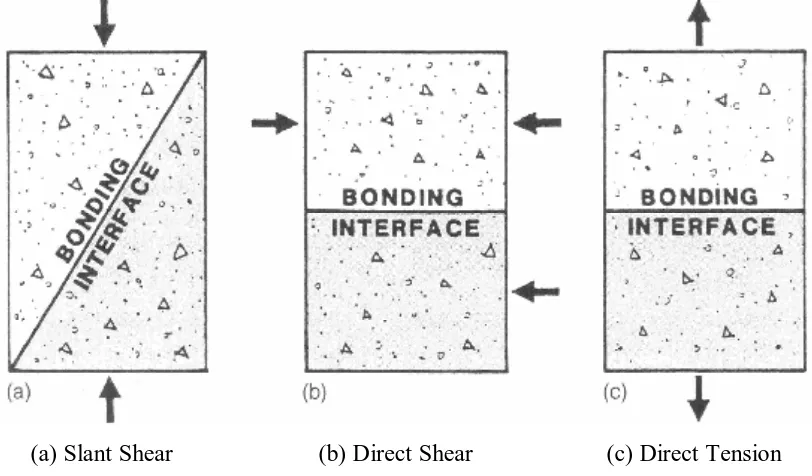
(a) Slant Shear (b) Direct Shear (c) Direct Tension Figure 2-2 Methods for testing bond strength (Hindo 1990)
Other testing methods exist such as those discussed by Wall et al (1986) where it was found that the slant shear test is the most accurate and least variable method of testing bond strength between two concrete layers, however it should be noted that the authors were only considering methods that involve both laboratory preparation and testing. The other tests conducted were an indirect tension test and flexural type test. For similar reasons as the slant shear tests, the other tests use specimens that could not be obtained from the field.
Another means of testing the bond strength used in the literature is the pull-off test. The pull-off test is a form of the Direct Tension but modified. Instead of completely coring a specimen and testing it in the laboratory, the specimen is only partially cored; specifically it is cored completely through the topping layer and partially into the original layer. Therefore, both production and testing of the specimen are conducted in the field.
method are Talbot et al (1994), Austin et al (1995), Cleland & Long (1997), and Júlio et al (2004). It appears to be the most common test method in use.
With regard to the other test methods, the next most common is the slant shear test. According to Emmons (1993), this method is prone to overestimating the actual bond strength, particularly since it is a laboratory only test. Júlio (2004), which used both the slant shear and pull-off tests, found that a direct correlation between the two tests exists. The factor was determined to be 0.1855, indicating the slant shear tests resulted in bond strengths over five times that of the pull-off tests.
In this experimental program, it was decided to use the direct tension test method to determine the concrete-to-concrete bond strength, where the top layer of concrete simulates the cast-in-place topping reinforced with C-Grid and bottom layer simulates the Precast DT. One of the goals of this research, namely to determine whether C-Grid deflects from its placed position during casting of the topping, requires the entire profile of the core to be visible and undamaged. The pull-off method would destroy the core before it could be examined. Another reason for using the direct tension method is that it is easier to ensure each test is conducted in similar (laboratory) conditions.
2.4 TESTING LONGITUDIONAL SHEAR STRENGTH
(a) push-off (b) pull-off (c) modified push-off Figure 2-3 Single-shear test specimens diagram (Mattock & Hawkins 1972)
2.5 SHEAR-FRICTION MODELS
This section of the literature review will focus on models for the shear capacity of a steel reinforced concrete section. They are often referred to as friction (or shear-transfer) models.
The models presented here will be later modified for the purposes of this research in Chapter 6. The motivation for reviewing these shear-friction models is to use them to predict the shear strength of C-Grid reinforced concrete, despite the fact that these were originally developed for steel reinforced concrete.
A typical shear-friction model considers a cracked concrete element (along the line of shear) in which the two concrete faces slip against one another due to the applied shear force. The amount of resistance due to friction depends on the roughness of the cracked concrete faces as well as the magnitude of the normal force acting on the concrete element. In this case, compressive normal forces will contribute to the shear-friction resistance, while tensile normal forces will reduce it. One component of this normal force is the axial strength of the transverse reinforcement. As the cracked concrete faces begin to slip, they also begin to dilate. This will induce tension in the reinforcement as it resists the crack dilation. As a result, in order to maintain equilibrium, there is a resultant compressive force normal to the cracked concrete faces. This can be thought of as a passive or internal normal force. Active or externally applied forces normal to the cracked concrete faces are another potential component of overall normal force. Although these components come from different sources (internal or external), they both affect the shear resistance through shear-friction. It should also be noted that dowel action, in which the reinforcement resists the applied shear force as it deforms along the shear plane, may also be included in the shear-friction model.
2.5.1 ACI 318-08
Vn = Avf yf µ [2-1]
were Vn is the nominal shear strength of the section, Avf is the area of shear reinforcement, fy is the yield strength of the shear reinforcement, with a limit specified by the code of 413.7 MPa (60,000 psi), and μ is the coefficient of friction as described in Eq. [2-2] below. Although it is not directly stated in the design equation, a strength reduction factor φ of 0.65 is applied for design. The coefficient of friction is determined by the manner in which the concrete plane in shear was constructed:
1.4 Concrete placed monolithically
1.0 Concrete placed against hardened concrete with surface intentionally roughened. 0.6 Concrete placed against hardened concrete
not intentionally roughened. 0.7 Co
λ λ
µ = λ
λ ncrete anchored to structural steel by headed studs or reinforcing bars
[2-2]
where λ is a correction factor related to the unit weight of concrete, which is taken as 1.0 for normalweight concrete.
In addition, the ACI 318 code specifies two upper limits to the shear strength, which are: ' 0.2 800 c c c
Vn f A
Vn A
≤
≤ [2-3]
where Ac is the area of the concrete section resisting shear transfer. The code commentary states the reason for this limit is that Eq. [2-1] becomes un-conservative at higher values.
Although the primary design equation is dimensionally correct, the limit states are not, so it is important to either only use the prescribed units of inches and pounds or otherwise alter the equations for SI metric units.
2.5.2 6th Edition of the PCI Design Handbook
Another shear-friction model is presented in the sixth edition of the Precast/Prestress Design Handbook PCI (2004) §4.3.6. Like the previous model in Section 2.5.1 this model does not account for the strength of the concrete in its determination of shear force being transferred. In addition, the model is not dimensionally correct and requires modification in order to use units other than inches and pounds. Lastly the model equation is setup to give a minimum area of shear reinforcement for a given ultimate shear force with appropriate safety factors, as opposed to solving for a resistance with a known or assumed amount of reinforcement. The equation is:
1000 u vf y e cr e u V A f A V = φ µ λ µ µ = [2-4]
where φ is the strength reduction factor, Avf is the area of reinforcement, fy is the yield strength of the reinforcement with a limit of 413.7 MPa (60,000 psi), Vu is the applied factored shear force, μ and μe are shear-friction coefficients, and Acr is the area of the crack interface.
The PCI model further defines the shear-friction coefficients based on the method of concrete placement at the point of shear transfer. The coefficient μ is defined as:
1.4 Monolithically cast concrete
1.0 Concrete to hardened concrete with roughened surface 0.6 Concrete to concrete
0.7 Concrete to steel
where λ is a factor for use with lightweight concrete (i.e. λ = 1.0 for normalweight concrete). The coefficient μe is given an upper bound limit based on the crack interface condition:
3.4 Monolithically cast concrete
2.9 Concrete to hardened concrete with roughened surface 2.2 Concrete to concrete
2.4 Concrete to steel
e ≤ ≤ µ = ≤ ≤ [2-6]
In the PCI model, no upper bound limit for the shear force is given.
2.5.3 Mattock et al
Another model which has been introduced and developed in the literature is a model first seen in Mattock & Hawkins (1972), which was based off of research done by Hofbeck et al (1969); and further studied by Mattock et al (1975).
Hofbeck et al (1969) used push off specimens (see Figure 2-3 for an illustration) to test the shear transfer along a plane of concrete. Though no design model was presented, the authors observed three things. First, they felt that concrete strength did not play a significant role in the overall shear transfer strength. Secondly, they found that an increase in the amount of reinforcement resulted in a proportional increase in shear strength except (and this is their third finding) up to a certain point. Therefore, they proposed an upper bound limit that is governed by the concrete strength.
These conclusions were reached again in Mattock & Hawkins (1972) which sought to model the shear transfer of concrete using a variety of single-shear type push off and pull-off specimens, as illustrated in Figure 2-3 from the paper. Many of the specimens and graphs published in this article originated from Hofbeck et al (1969).
Based off these results, an equation was developed to model the shear transfer across a crack in monolithic concrete:
200 0.8( )
u y Nx
v = psi+ pf + σ [2-7]
applied direct stress perpendicular to the shear plane. The value of 200 psi is the contribution to shear resistance that the (cracked) concrete plane along the shear plane will provide (presumably through friction and aggregate interlock).
Along with this there is an upper bound imposed on this model that is: '
0.3
u c
v ≤ f [2-8]
where fc’ is the compressive strength of the concrete.
Also, a restriction on the sum of the reinforcement strength parameter pfy and externally applied force parameter σNx is imposed:
200
y Nx
pf + σ ≥ psi [2-9]
This is justified by the understanding that an insufficient amount of force being applied normal to the plane of shear transfer will result in a lower than expected contribution to the shear resistance by the friction of the concrete, which itself is set as a fixed 200 psi in Eq. [2-7].
Figure 2-4 Comparison of shear-transfer strength (Mattock & Hawkins 1972)
Figure 2-5 Effect of concrete strength on shear-transfer (Mattock & Hawkins 1972)
The authors explain that, beyond vu of 700-800 psi, the strength of the concrete (or lack thereof) causes the relationship between vu and pfy to break down. This is why the authors proposed an upper limit to vu of 0.3fc’ (see Eq. [2-8]), which in the case of the fifth series (in Figure 2-5), is 750 psi, about where the two series begin to deviate. Below this upper bound cut-off, the behavior between the two series of specimens is the same, despite different concrete strengths. So in effect, the authors are saying that the shear transfer strength becomes dependent on the concrete strength after a certain point.
Also, consider that a design equation should always consider a cracked concrete interface – as the authors noted – since any number of things not related to the applied load can cause the section to crack, such as shrinkage or handling.
This model is used again by Mattock et al (1975) to predict the behavior of initially cracked concrete both with and without the direct shear stress term σNx. In this paper, the experimental specimens were corbels (as seen in Figure 2-6) and push off specimens as seen in Figure 2-3a.
Figure 2-6 Corbel type push off specimen (Mattock et al 1975)
However, the paper used a different equation; the reason for this seems to be modifying the model to calculate the mean strength, as opposed to producing a conservative (characteristic) design equation. The modified equation is:
400 0.8( )
u y Nx
This can be seen by the graph of this altered model versus the experimental data in Figure 2-7. One can see the plotted curve of the altered model goes roughly down the center of the experimental scatter, as opposed to a design model which would be expected to be a lower bound of the scatter in order to be conservative. This demonstrates that the equation can be modified relatively easily to suit different purposes; which is done in future work by Oehlers & Bradford (1995, 1999).
2.5.4 Oehlers & Bradford
This shear-transfer model across concrete is further studied and modified in two separate books by Oehlers & Bradford (1995 and 1999) which refers to the work from Section 2.5.3 as the Mattock Model. The first book (1995) introduces different nomenclature to the Mattock model from Mattock & Hawkins (1972) and adapts it to SI metric units of N and mm. The adapted equation takes the form:
( )
1.4 MPa 0.8 0.8
u ch lock dow fric
lock
dow yr
fric nf
v v v v
v v pf v = + + = = = σ [2-11]
where vlock is the strength attributed to interface interlock, vdow is the dowel resistance, vfric is the active frictional resistance, and (vu)ch is the characteristic (design) shear strength of a cracked shear plane, σnf is the stress normal to the shear plane, and pfyr is the yield stress of the reinforcing material per unit area of the shear plane.
The book proceeds to make several modifications and additions to the Mattock model. The first is the modification of the vlock term to – instead of being a constant value of 1.4 MPa (200 psi) –a function of the tensile strength fct.
This is reasonable considering how much the understanding of aggregate interlock has progressed from the time of the original publishing of the Mattock model (1972) to the writing of Oehlers & Bradford (1995). Recall that Hofbeck et al (1969) and Mattock & Hawkins (1972) observed that concrete strength became a factor at a certain shear strength value; therefore, it would be reasonable to allow the concrete strength to be a factor for any shear strength value. The book considers the tensile strength of the concrete to be the primary contributor to aggregate interlock forces. Therefore, the term for vlock becomes:
0.66
lock ct
v = f [2-12]
(1.4 MPa) for vlock and a concrete strength of predominately 4000 psi (27.6MPa). Substituting 27.6 MPa for fc’ in Eq [2-12] results in a vlock of 1.4MPa. This factor of 0.66, which was not given a name by Oehlers & Bradford, is defined for convenience as the concrete/statistical coefficient Γ for the purposes of this literature review and research.
Oehlers & Bradford (1995) further developed the original Mattock model by deriving different values of Γ for different scenarios and statistical considerations. For instance, in Mattock et al (1975) as discussed in the previous Section, the Mattock model can be easily changed to predict the mean (average) values as opposed to calculating lower bound characteristic (design) values. Oehlers & Bradford (1995) adequately changed the Mattock model from a characteristic (design) to a mean model by using a value of 1.1 for Γ.
In addition to that, the strength of an uncracked concrete shear plane (note all previous values were under the assumption of a cracked concrete shear plane) can be arrived at by using a Γ of 1.6. Therefore, the model can be used in many applications for both predicting actual (mean) strength or as a conservative design model (characteristic) for cracked and uncracked situations as given in Table 2-2. Note that there is no Γ value for the characteristic uncracked condition. This is because it would be imprudent to design with the assumption that the shear resisting concrete section will remain uncracked for its service life, an inherently un-conservative assumption.
Table 2-2 Adaptation of the Mattock model to different circumstances Concrete Condition Mean Characteristic
Initially Cracked Γ = 1.1 Γ= 0.66 Initially Uncracked Γ = 1.6 N/A
as given by the following expression but indirectly describe what happens when the lower bound, which is given in Eq. [2-13], is not met.
0.66
yr nf ct
pf + σ ≥ f [2-13]
Below this lower bound, Oehlers & Bradford show the shear strength decreasing in a parabolic manner to zero when pfyr is zero. The graph is reproduced in Figure 2-8 and the region in question is the dashed-line parabola 0B. Note a similar parabolic curve from Mattock et al (1975) in Figure 2-7. The point of the lower bound limit is point B where the parabola and the linear portion BC intersect. Note that as the parabola 0B approaches point B, the slope approaches that of the slope of the line BC.
Figure 2-8 Modified Mattock model (Oehlers & Bradford 1995)
Oehlers & Bradford (1999) is a continuation of their previous work that presents one more modification to the Mattock Model. That is simply transforming the equation to a per unit length basis. The model is now written in terms of shear flow given by:
0.66 0.8 0.8
ch ct p tr yr nf
Q = f L + A f + F [2-14]
where Qch is the shear flow strength, fct is the tensile strength of the concrete, Lp is the depth of the shear plane, Atr is the area of transverse reinforcement per unit length, fyr is the yield strength of the transverse reinforcement, and Fnf is the normal force per unit length. A specific definition for fct, using units of N and mm, is given as:
' 0.4
ct c
f = f [2-15]
The upper limit is rewritten as: ' 0.3
ch c p
Q ≤ f L [2-16]
0.8(A ftr yr +Fnf)≥0.53f Lct p [2-17]
Equation [2-17] can be simplified and written as: 0.66
tr yr nf ct p
A f +F ≥ f L [2-18]
Finally, Eq. [2-14] can be rewritten to include the modifications of Oehlers & Bradford (1995), mainly the introduction of the concrete/statistical coefficient Γ as introduced in Table 2-2:
0.8 0.8
where:
0.66 characteristic strength of cracked concrete 1.1 mean strength of cracked concrete, 1.6 mean strength of uncracked concrete
ch ct p tr yr nf
Q = Γf L + A f + F
Γ =
[2-19]
CHAPTER 3 EFFECT OF C-GRID ON THE COLD JOINT BOND
3.1 INTRODUCTION
In this Chapter, two objectives are addressed regarding the feasibility of the use of Carbon Fiber Grid (C-Grid) instead of Welded Wire Fabric (WWF) as reinforcement in cast-in-place topping slabs of Precast/Prestressed Double Tee (Precast DT) systems. The first is to determine the amount, if any, that C-Grid may deflect vertically during casting of the topping on top of the Precast DT. This effect will be referred to as “floating”. This is of concern because C-Grid is a very light material, approximately 10% the density of steel. It is also flexible and not likely to be restrained against upward or downward deflection. If the C-Grid floats too much from its expected position, then calculations (such as flexural analysis) which assume the C-Grid is at its original placed location will obviously be inaccurate.
The second objective is to determine the amount, if any, that the location of the C-Grid during casting of the topping compromises the cold joint bond (interface) between the two layers of concrete cast at different times. This is of concern since the quality of the bond affects the integrity of the structural floor system and the ability of it to provide adequate diaphragm action. In that case, there might be a concrete cover requirement for sufficient concrete to concrete (cold joint) bond.
These objectives are achieved primarily by cored direct tension tests, which are utilized to test the bond strength of the cold joint bond for reasons discussed in Section 2.3.3. The use of cored cylinders from a C-Grid reinforced slab allows its profile to be observed visually to inspect for floating of the C-Grid reinforcement.
3.2 MATERIALS AND METHODS
3.2.1 Casting of Slabs
a typical specified concrete strength of fc’ = 34.5 MPa (5000 psi) and thickness t = 90 mm (2.75 in). The bottom layer was given a surface roughness finish of CSP-4 (as discussed in Section 2.3.1. The top layer simulates the cast-in-place topping, with a typical specified concrete strength of fc’= 20.7 MPa (3000 psi) and thickness t = 70 mm (2.75 in). The top layer was cast four weeks after the first. Before the top layer was cast, the surface of the bottom layer was wetted to a degree such that there was no standing water on the surface before casting. Given the hot temperatures in which the top layer was cast – approximately 32-35 ºC (90-95 ºF) – this pre-wetting was deemed important, as discussed in Section 2.3.2.
Before casting of the top layer, several sizes of C-Grid (see Table 3-1 and Figure 3-1) were placed on top of the bottom layer using various chairing or restraining methods as shown in Figure 3-2 and Figure 3-3. The C-Grids were placed in intervals along the slab to allow for thirteen different variations including two controls of plain concrete topping (no C-Grid reinforcement). A schematic of the two slabs, Slab 1 and Slab 2, is shown in Figure 3-4 and Figure 3-5 shows the actual slabs with the bottom layer of concrete cast and the C-Grid reinforcement in place, awaiting the top layer of concrete.
The four sizes of C-Grid, in order of increasing strand spacing and hence lower reinforcement ratios, are C50 1.6x1.8, C50 2.2x2.2, C50 2.9x2.9, and C50 3.5x4.0 (as the strength properties of the Grid are not critical here, they are given in Chapter 4). These Grids are representative of those used in current applications. For comparative purposes, C-Grids with relatively lower or higher strand spacing (and hence higher or lower reinforcement ratios) are referred to as being more or less dense, respectively.
10 mm (0.4 in). Two different shapes were used, Figure 3-3 illustrates the different shapes, which for convenience are referred to as flat cylindrical rubber chairs (“flat chair” or “FC”) and roller shaped rubber chairs (roller chair or “RC”). The fifth method simply used a ferris-wheel shaped plastic chair (“ferris-wheel chair or “WC”) normally used to chair steel WWF by 25 mm (1 in).
Laying the C-Grids flat with no restraint would be the quickest and cheapest way of placing the C-Grid; however, this is also likely to be more susceptible to floating. Chairing options are being considered because the C-Grid will be offset from the interface of the two concrete layers, likely reducing the affect on the bonded interface. However, the chaired C-Grid may “float” both up or down from its initial position during casting.
Table 3-1 C-Grid dimensional properties C-Grid Designation Longitudinal Spacing† mm (in) Transverse Spacing† mm (in) C50 - 40x44
(C50 - 1.6x1.8)
40.64 (1.6)
45.72 (1.8) C50 - 56x56
(C50 - 2.2x2.2)
55.88 (2.2)
55.88 (2.2) C50 - 72x72
(C50 - 2.9x2.9)
73.66 (2.9)
73.66 (2.9) C50 - 89x102
(C50 - 3.5x4.0)
(a) C50 1.6 x 1.8 (b) C50 2.2 x 2.2
(c) C50 2.9 x 2.9 (d) C50 3.5 x 4.0
(a) “NR” No Restraint, C-Grid laid flat (b) “HG” C-Grid secured by Hot Glue (c) “FC” Flat cylindrical rubber Chairs
(a) “FC” type
(b) “RC” type
(a) Slab 1
(b) Slab 2
3.2.2 Coring of Specimens
(a) Core locations marked and numbered
(b) Specimens being cored
Table 3-2 Schedule of cores
Specimen No. C-Grid Restraint Specimen No. C-Grid Restraint
A1 C50 2.9x2.9 WC A22 C50 1.6x1.8 NR
A2 C50 2.9x2.9 WC A23 C50 1.6x1.8 NR
A3 C50 2.9x2.9 WC A24 C50 1.6x1.8 NR
A4 C50 3.5x4.0 FC A25 C50 2.2x2.2 NR
A5 C50 3.5x4.0 FC A26 C50 2.2x2.2 NR
A6 C50 3.5x4.0 FC A27 C50 2.2x2.2 NR
A7 C50 3.5x4.0 RC A28 C50 2.9x2.9 NR
A8 C50 3.5x4.0 RC A29 C50 2.9x2.9 NR
A9 C50 3.5x4.0 RC A30 C50 2.9x2.9 NR
A10 C50 2.9x2.9 HG A31 C50 3.5x4.0 NR
A11 C50 2.9x2.9 HG A32 C50 3.5x4.0 NR
A12 C50 2.9x2.9 HG A33 C50 3.5x4.0 NR
A13 C50 3.5x4.0 HG A34 C50 1.6x1.8 HG
A14 C50 3.5x4.0 HG A35 C50 1.6x1.8 HG
A15 C50 3.5x4.0 HG A36 C50 1.6x1.8 HG
A16† None N/A A37 C50 2.2x2.2 HG
A17† None N/A A38 C50 2.2x2.2 HG
A18† None N/A A39 C50 2.2x2.2 HG
A19† None N/A
A20† None N/A
A21† None N/A
†
3.2.3 Experimental Procedure
Around the circumference of the cored cylinder it is possible to identify and measure the level of both the cold joint (interface) plane between the two concrete layers (which appears as a line between two different textures of concrete) and the plane of the C-Grid strands (which appear in cross-section) in the top layer. Therefore, the edge-to-edge distance between the C-Grid and the cold joint was measured at four equally spaced points along the circumference of each cylinder (see Figure 3-7). For each cylinder, the four values are averaged and this value is termed the “final location”. The float (vertical displacement as a result of the casting process) is quantified by comparing the final location with the “initial location”, which depends on the restraining method used.
Figure 3-7 Measuring C-Grid float in cores
which consist of a flat 152.4 mm (6 in) diameter base welded to a 25.4 mm (1 in) diameter rod with stiffeners (Figure 3-8), were epoxy glued to the top and bottom face of the specimen. So that the epoxy may cure properly and to ensure vertical alignment of the steel attachments, (to produce pure axial load) a steel frame jig (Figure 3-9) was used to secure the specimen while the epoxy cures. The epoxy was allowed to cure for a minimum of 72 hours prior to testing as seen in Figure 3-10. A schematic of the finished specimen is illustrated in Figure 3-11. Each specimen was then tested in an MTS testing machine to apply a direct tension force to the core (Figure 3-12).
(a) Specimen loaded in MTS (b) Specimen failure in MTS Figure 3-12 Specimen in MTS machine
3.3 RESULTS
3.3.1 C-Grid Floating
The initial location of the C-Grid is 0 mm for HG and NR restraints (since they are laid flat on the concrete surface), 25.4 mm (1 in) for WC, and 9.5 mm (0.375 in) for FC and RC relative to the interface.
as the extreme values (maximum, minimum, and the difference between the two). Appendix A contains the raw data for the C-Grid final locations and float calculations.
Note that, because specimen A4 (one of the three C50 3.5x4.0 flat chair specimens) is so different from the rest of the specimens of that sample (and indeed, of all the cores), the calculations for 3.5x4.0 FC are repeated twice in the table. The entry with an asterisk (*) is calculated without specimen A4 included as it can be considered an outlier. It is apparent by visual inspection of this specimen that the plane of the C-Grid strands is considerably eccentric as opposed to parallel with the plane of interface as was the case with all other specimens.
Figure 3-13 is a graphical representation of the initial and final location of the C-Grid scaled relative to the actual size of the cores, that is, the vertical axis spans 140 mm (5.5 in) which is the overall height of the cored cylinders with 0 mm being the interface between the two concrete layers.
Table 3-3 Float results summary
Specimen Set Average Float mm Standard Deviation mm Float as % of 70mm† Max mm Min mm
(Max - Min) mm
(Max - Min) as a % of 70mm
1.6x1.8 NR 3.08 1.23 4.4% 6 1.5 4.5 6.4%
2.2x2.2 NR 5.08 0.40 7.3% 7.5 4 3.5 5.0%
2.9x2.9 NR 4.54 1.04 6.5% 6.5 1.5 5 7.1%
3.5x4.0 NR 1.50 0.38 2.1% 2 0.5 1.5 2.1%
1.6x1.8 HG 2.92 0.26 4.2% 4 1.5 2.5 3.6%
2.2x2.2 HG 1.96 0.19 2.8% 3 1 2 2.9%
2.9x2.9 HG 4.21 0.88 6.0% 7 2 5 7.1%
3.5x4.0 HG 1.38 0.13 2.0% 2.5 0.5 2 2.9%
3.5x4.0 FC -0.83 8.24 -1.2% 19 -8 27 38.6%
3.5x4.0 FC* -5.83 1.33 -8.3% -2.5 -8 5.5 7.9%
3.5x4.0 RC -5.75 1.31 -8.2% -1 -7 6 8.6%
2.9x2.9 WC -12.75 3.15 -18.2% -3 -17.5 14.5 20.7% *
Specimen A4 excluded †
3.3.2 Direct Tension Tests
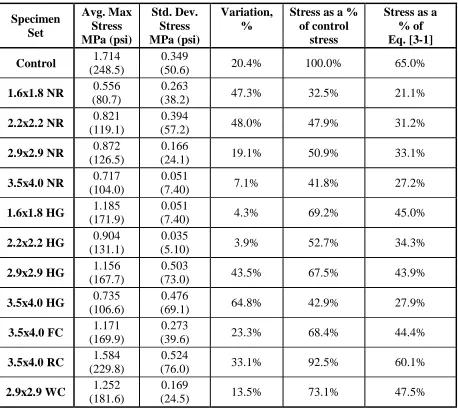
Appendix B contains the raw data for the breaking (maximum) load and stress of each individual core along with the average stress and average stress as a percentage of the control stress for each specimen set. Table 3-4 summarizes the tension test data and includes: average stress, standard deviation of stress, the percentage variation (standard deviation divided by average stress), the stress as a percentage of the average control stress (no C-Grid), and the stress as a percentage of the tensile strength of concrete used in the topping.
The tensile strength can be found by using the following equation from ACI 318-08: 6
t c
f′= f′ . [3-1]
Note Eq. [3-1] is not dimensionally correct and requires the use of psi units. From Appendix C, the compressive strength of concrete was determined to be fc’ = 28.01 MPa (4062 psi) for the top layer and fc’ = 50.41 MPa (7312 psi) for the bottom layer. Since the upper layer is the weaker of the two, it controls; this results in a tensile strength ft’ = 2.65 MPa (382 psi) according to Eq. [3-1].
Figure 3-14 contains a graph of tensile stress on the ordinate and the specimens arranged on the abscissa according to the C-Grid spacing in the given specimen. Also shown as lines is the average tensile stress of the control stress and the ACI 318-08 tensile strength. Figure 3-15 combines both the average stress from this section and average final positions from Table 3-3. Other graphs were produced in order to determine if the tensile (bond) strength is influenced by the following characteristics: C-Grid size (Figure 3-14), C-Grid restraint (Figure 3-14), or the final location (Figure 3-15).
Table 3-4 Tension test summary Specimen Set Avg. Max Stress MPa (psi) Std. Dev. Stress MPa (psi) Variation, %
Stress as a % of control
stress
Stress as a % of Eq. [3-1] Control 1.714
(248.5)
0.349
(50.6) 20.4% 100.0% 65.0%
1.6x1.8 NR 0.556 (80.7)
0.263
(38.2) 47.3% 32.5% 21.1%
2.2x2.2 NR 0.821 (119.1)
0.394
(57.2) 48.0% 47.9% 31.2%
2.9x2.9 NR 0.872 (126.5)
0.166
(24.1) 19.1% 50.9% 33.1%
3.5x4.0 NR 0.717 (104.0)
0.051
(7.40) 7.1% 41.8% 27.2%
1.6x1.8 HG 1.185 (171.9)
0.051
(7.40) 4.3% 69.2% 45.0%
2.2x2.2 HG 0.904 (131.1)
0.035
(5.10) 3.9% 52.7% 34.3%
2.9x2.9 HG 1.156 (167.7)
0.503
(73.0) 43.5% 67.5% 43.9%
3.5x4.0 HG 0.735 (106.6)
0.476
(69.1) 64.8% 42.9% 27.9%
3.5x4.0 FC 1.171 (169.9)
0.273
(39.6) 23.3% 68.4% 44.4%
3.5x4.0 RC 1.584 (229.8)
0.524
(76.0) 33.1% 92.5% 60.1%
2.9x2.9 WC 1.252 (181.6)
0.169
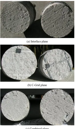
(a) Interface plane
(b) C-Grid plane
Table 3-5 Failure plane profiles Specimen Set Specimen No. Failure Profile† Specimen Set Specimen No. Failure Profile† 2.9x2.9 WC 1 Interface 1.6x1.8 NR 22 Combined 2.9x2.9 WC 2 Interface 1.6x1.8 NR 23 Combined 2.9x2.9 WC 3 Combined 1.6x1.8 NR 24 Interface
3.5x4.0 FC 4 Interface 2.2x2.2 NR 25 Interface 3.5x4.0 FC 5 Interface 2.2x2.2 NR 26 Interface 3.5x4.0 FC 6 Combined 2.2x2.2 NR 27 Interface
3.5x4.0 RC 7 C-Grid 2.9x2.9 NR 28 Interface
3.5x4.0 RC 8 C-Grid 2.9x2.9 NR 29 Interface
3.5x4.0 RC 9 Interface 2.9x2.9 NR 30 Interface 3.5x4.0 HG 10 Combined 3.5x4.0 NR 31 Combined 3.5x4.0 HG 11 Combined 3.5x4.0 NR 32 Combined 3.5x4.0 HG 12 Combined 3.5x4.0 NR 33 Combined 2.9x2.9 HG 13 Interface 1.6x1.8 HG 34 Interface 2.9x2.9 HG 14 Combined 1.6x1.8 HG 35 Combined 2.9x2.9 HG 15 Combined 1.6x1.8 HG 36 Combined Control 16 Interface 2.2x2.2 HG 37 Interface Control 17 Interface 2.2x2.2 HG 38 Combined Control 18 Interface 2.2x2.2 HG 39 Interface
Control 19 Interface
Control 20 Interface
Control 21 Interface †
See Figure 3-16
3.4 DISCUSSION
3.4.1 C-Grid Float
Core four, which is an outlier, is believed to be caused by disturbance during construction. The concrete vibrator or a concrete shovel could have easily shifted the C-Grid in the area around the core out of place. Caution must be observed when casting C-Grid reinforced concrete, including ensuring that all concrete tools do not impact the C-Grid. Excluding the outlier, the largest individual specimen float was +5.38 mm (0.211 in).
Both the No Restraint and the Hot Glue specimens maintained their position very well. Interestingly enough, there is not a lot of difference in float between the various C-Grid sizes as well as the two restraint methods themselves. C-Grid sizes 1.6x1.8 and 3.5x4.0 performed the best while 2.2x2.2 and 2.9x2.9 floated a few millimeters more. Considering though that the largest float was 5.4 mm (0.21 in) individually and 5.1 mm (0.20 in) on average, it can be said that float is not a concern with these methods of restraint and with all of these C-Grids since 5.4 mm and 5.1 mm are 7.7% and 7.3% of the height of the top layer of concrete, respectively. If one desires to place the C-Grid flat against the surface of the Precast DT, there really is not a need to Hot Glue (or otherwise secure) the C-Grid.
The chairing methods of restraint all suffered, to varying degree, from downward movement from their initial location. This is most likely caused by the weight of the concrete bearing down on the C-Grid. In the case of the RC and FC chairs, the weight of the concrete also has the potential to compress the rubber chairs. Overall, this downward movement should not pose much of a problem as long as the chairs are closely spaced. It is possible that the experiment exaggerated this effect since only 0.30 by 1.22 m (1 by 4 ft) strips of C-Grid were used in the Slabs, as opposed to a continuous roll of C-Grid. All of them deflected to approximately just over halfway between the intended location and the interface line. The FC chaired C-Grids floated, on average, -5.83 mm from an initial height of 10 mm (58.3%), the RC chaired C-Grids floated -5.75 mm from 10 mm (57.5%), and the WC chaired C-Grid floated -12.75 mm from 25 mm (51.0%).
test fair, no one was allowed to step on the slabs during casting, however in a practical application construction workers would have to walk on the top of the Precast DT and would end up stepping on the C-Grid. This is another reason to recommend against the use of wheel chairs. As the RC and FC chairs are constructed of flexible rubber and are only 10 mm in height, they are far less susceptible to damage from construction and being stepped on.
3.4.2 Direct Tension Tests
As a result of having two layers of concrete with a cold joint, the strength drops 35% from the ACI 318-08 tensile strength (if the core was one uniform layer instead of two). In addition, having any form of C-Grid drops the strength further, ranging from 21% to 60% of f t’.
When the specimens were broken, the two faces where failure had occurred were observed and pictured (samples of which are shown in Figure 3-16). In many of these, it was clear where the C-Grid had interfered with the concrete paste from the top layer being able to flow under the C-Grid and bond to the existing layer of concrete. The evidence is the discoloration/indentation of the bottom surface matching the shape of the C-Grid and the voids that appear in this region (unlike the rest of the failure plane, which was compacted well). This does not occur in Figure 3-16(a) since that was a specimen with no C-Grid. This could certainly be responsible for the reduction of the bond strength of the cold joint.
Based on Figure 3-14, the strength varies on the type of restraint used rather than the type of C-Grid used. For instance, all the Hot Glue specimens are (by varying amounts) stronger than the No Restraint specimens. In addition, all the chaired specimens are stronger than any non-chaired C-Grids. The best performer was the Roller Chairs at 93% the control strength. Conversely, when looking at just C-Grid size, no apparent trend was observed.
varying amounts, on all of these factors combined (C-Grid size, height, and restraint method).
Lastly, one should notice the considerable range of values of the peak load for specimens of the same C-Grid size and restraint. Variations range from 4% to 65%, with the average being 27%. This suggests that bond strength can contain localized weak spots and that quality control is very important, specifically ensuring compaction near the interface of both layers of concrete.
CHAPTER 4 LONGITUDINAL SHEAR-SLIP BEHAVIOR OF C-GRID REINFORCED CONCRETE
4.1 INTRODUCTION
The objective of this Chapter is to quantify the effect of Carbon Fiber Grid (C-Grid) on the longitudinal shear strength and shear-slip relationship of a cast-in-place concrete topping of a Precast/Prestressed Double Tee (Precast DT) system using small-scale single-shear tests to determine the fundamental longitudinal single-shear-slip response. Since the longitudinal joint between two Precast DT sections is the weakest plane, this experiment focuses on the longitudinal shear strength at this location. Various C-Grid sizes and orientations of C-Grid (the angle of the C-Grid fibers relative to the line of shear) were tested.
4.2 MATERIALS AND METHODS
4.2.1 Specimens
was cast with a discontinuity (gap) along the line of shear. This gap, which was about 3 mm (1/8 in) in width, represents the joint between the two Precast DTs. The top layer simulates the cast-in-place topping, with a specified concrete strength of fc’ = 20.7 MPa (3000 psi) and thickness t = 70 mm (2.75 in). The top layer was cast four weeks after the first layer was cast. As was described in Chapter 3, the surface of the bottom layer of concrete was pre-wetted, but no standing water was present when the top layer of concrete was cast (recall the discussion from Section 2.3.2). Note that the specimens of this Chapter were constructed at the same time as the Slabs of Chapter 3 and with the same batches of concrete for the top and bottom layers. However the measured concrete strengths were slightly different given that specimens A1-A39 from Chapter 3 were tested at a different time then specimens B1-B10 of this Chapter, see Appendix A.
The result is a specimen in which only the top layer of concrete (the topping) and C-Grid reinforcement resist the shear force. This set up assumes the Precast DT shapes are not connected together in any way (effectively the tests represent a worst-case scenario).
Before casting of the top layer, several sizes (the same sizes from Chapter 3) and orientations of C-Grid were placed flat on top of the bottom layer of concrete (restraint method “NR”, from Figure 3-2). Combining this and the surface layer roughness applied to the top of the bottom layer the Reinforcement Placement Method can be termed (for future reference) as NR-CSP-4 for these single-shear tests. Details of the dimensional and material properties of Grid are found in Table 3-1 and Appendix D, respectively (note that the C-Grid used in this series of tests was from the same batch used throughout this research).
Figure 4-2 illustrates the various C-Grid orientations used in rectangular and square C-Grids, respectively. Rectangular C-Grids (C50 - 1.6x1.8, C50 - 3.5x4.0) are those with unequal strand spacing in the transverse and longitudinal direction, hence a “strong” and “weak” orientation. Square C-Grids (C50 – 2.2x2.2, C50 – 2.9x2.9) are those with equal strand spacing in both directions, and can be placed so that the strands are oriented at a 0º/90º angle or a ±45º angle, hence “perpendicular” and “diagonal” orientations, respectively. Note that, with regard to the number of strands crossing the shear line and diagonally oriented C-Grids, all strands crossing were counted, regardless if the strand was +45 º or -45º, the reason for this is explained in Appendix D. Also note that specimens with identical C-Grid size and orientation have the same number of strands crossing the shear line (for example, B2 and B5 both have C50 2.2x2.2 oriented perpendicularly and have eight strands crossing the line of shear).
Table 4-1 Shear specimen schedule
Specimen C-Grid Top Layer of Concrete
Orientation of C-Grid
Strands Crossing Shear Line
B1 (ctrl) None Continuous None N/A
B2 (ctrl) C50 2.2x2.2 Discontinuous Perpendicular 8
B3 C50 1.6x1.8 Continuous Strong 11
B4 C50 1.6x1.8 Continuous Weak 9
B5 C50 2.2x2.2 Continuous Perpendicular 8 B6 C50 2.9x2.9 Continuous Perpendicular 6
B7 C50 3.5x4.0 Continuous Strong 5
B8 C50 3.5x4.0 Continuous Weak 4
B9 C50 2.2x2.2 Continuous Diagonal 12
(a) Strong Orientation (more strands) (b) Weak Orientation (fewer strands) Figure 4-2 Rectangular C-Grid orientations