DataSlicer: Enabling Data Selection for Visual Data Exploration

DataSlicer: Enabling Data Selection

For Visual Data Exploration

Farid Alborzi, Rada Chirkova,

Pallavi Deo, Christopher Healey,

Gargi Pingale, Vaira Selvakani

Email: {falborz,rychirko,psdeo, healey,gpingal,vbselvak}@ncsu.edu

Juan Reutter

Pontificia Universidad Catolica de Chile Email: [email protected]

Surajit Chaudhuri

Abstract—Determining how to select and transform the data for visualization is one of the hardest problems faced by data-unfamiliar or inexperienced users when performing a visual exploration to solve an analytical task. Our main hypothesis is that for many data sets and common analytical tasks, such as finding outliers or general trends in data, there are relatively few “data slices” that are key to providing effective visualizations for the task. By focusing human users on appropriate and suitably transformed parts of the underlying data sets, these data slices can help the users carry their task to correct completion.

To verify this hypothesis, we develop a framework that permits us to capture exemplary data slices in an exploration task, and to explore and parse visual-exploration sequences into a format that makes them distinct and easy to compare. We develop a recommendation system, DataSlicer, that matches a “currently viewed” data slice with the most promising “next effective” data slices for the given exploration task. We report the results of controlled experiments with an implementation of the DataSlicer system, using four common analytical task types. The experiments demonstrate statistically significant improvements in accuracy and exploration speed versus users without access to our system.

I. INTRODUCTION

Data-intensive systems accompanied by visualization tools are being increasingly used for interactive data explorations [25], [26], [19], [22], [28], [18], [27]. These and other systems provide useful tools that help data analysts in their exploratory tasks of visually identifying trends, patterns, and outliers of interest. The visualizations make it more efficient to find task-relevant types of objects in exploratory data analysis, especially in presence of very large data. The reason is, visualizations allow analysts to leverage their domain expertise, knowledge of context, and ability to manage ambiguity in ways that a fully automated system cannot.

Due to the exploratory nature of their tasks, analysts often face a wide variety of visualization options to choose from. As pointed out in [28], it is not the visualization per se that is the main challenge. Indeed, once the data to visualize have been selected and transformed (e.g., grouped and aggregated in an appropriate way), users can take advantage of a visualization tool to provide an appropriate and effective visual presentation of the resulting data. In this paper we look into exploratory data analysis under the assumption that we have access to such presentationsolutions, and focus instead on the issue of determining which “data slices” would be the most helpful to the user in addressing the task at hand when visualized. Here,

the term data slice refers to the outcome of the process that involves selecting the data of interest from the given data set, as well as potentially applying transformations (e.g., grouping and aggregation) to the selected data.

The issue of identifying the data slices that are appropriate for the given task is a challenge for inexperienced users or those not familiar with the data at hand. The reason is that, typically, only a small fraction of the available data slices results in task-relevant visualizations, while all the other options fails to help the user with her task. This may force such users to examine a large number of options, to find those that lead to relevant visualizations for their exploration or analysis task. While clearly a challenge in presence of large-scale data, this is a hard problem even when the data set is small.

Our Focus: Our focus is on analytical tasks of common interest, such as detection of outliers or trends, that users often perform in visual exploratory analysis of data. Our objective is to improve the user experience by suggesting to her those data slices that, when visualized, present correct solutions to her task in a prominent way. Solving this problem would be instrumental in helping casual or inexperienced users to effectively conduct explorations of potentially unfamiliar data sets, in a number of application domains and for a spectrum of exploration objectives. For our study, we assume that a user begins work by declaring the task that she plans to perform. We also assume that she is able to identify a correct solution for her task (e.g., an outlier) when the solution is presented to her prominently in a visualization of some data slice.

Proposed Solution:We address the combinatorial explosion in data-slice selection by basing data-slice suggestions on the stage at which the user is in solving her task, and (when available) on expert knowledge of the domain, task, and data set. In this emphasis on, and appreciation of, expert knowledge in solving complex data problems, our effort is in line with the research directions such as that of DeepDive [21], [24].

As an illustration, consider a relational table storing infor-mation obtained from [4] (see [15] for the details) on major earthquakes worldwide from 1900 through 2013. The data set has 17 attributes and 8289 data points, please see Fig. 1(a) for a fragment of the data.

Place

AVG of Dep.

AVG of Mag.

NUM. of Rec.

Guadeloupe 100.0 7.4 1

Antigua and Barbuda

16.9 6.6 4

Martinique 102.0 7.0 3

East of Do-minica

11.2 7.2 1

(a) A fragment of the data set [4] (b) A visualization using dimensionsaverage mag-nitude(of earthquakes at location),number of earth-quakes(at location), anddepth(of earthquake)

(c) A visualization using only theaverage magnitude

dimension (bigger circles represent greater average magnitude)

Fig. 1. Visual exploration (part 1) in search of earthquake-magnitude outliers in Central America using data set [4], please see experimental task 1 in Section VII. The arrows in (b) and (c) highlight the visualizations of the “Guadeloupe” data point shown in (a); this data point is one of the answers to task 1.

(a) A visualization using the average magnitude di-mension (darker tones represent greater magnitude)

(b) Box plot showing outlier values of average earthquake magnitude

(c) A visualization showing the answers (magnitude-outlier earthquake locations) prominently on the map

Fig. 2. Visual exploration (part 2) in search of earthquake magnitude outliers in Central America using data set [4], please see experimental task 1 in Section VII. The sequence (b)–(c) is an expert solution to the task. The arrows in (a) and (c) highlight the “Guadeloupe” answer data point, please see Fig. 1.

to examine a map showing locations and other information about the earthquakes in the data set. One such visualization is shown in Fig. 1(b). The key point to note is that this visualization is unlikely to be helpful to those users who are not familiar with the data set. For instance, the arrow in Fig. 1(b) is pointing to one correct answer (Guadeloupe in Fig. 1(a)) for this exploration task; observe that the visualization is not conducive to finding that answer, as the data point in question does not stand out in the visualization.

One explanation for the relative ineffectiveness of the visu-alization of Fig. 1(b) for the exploration task at hand is that Fig. 1(b) shows not only the location and magnitude, but also other information about each earthquake. Suppose the analyst eliminates those features of the data that are irrelevant to the task at hand; the resulting visualization could be as in Fig. 1(c) or 2(a).1 _{Interestingly and perhaps counterintuitively, we have} found that these visualizations are not very helpful either to human viewers performing this task on the data set [4], again because the answers do not all stand out visually.

A more effective way to address this exploratory task is for the user to first examine a box plot showing the earthquake-magnitude mean and outlier whiskers; please see Fig. 2(b) for the visualization. Once the cutoff value for outlier earthquake magnitude has been found, the user can effectively construct a correct answer for her task by filtering out the irrelevant data. The result is visualized in Fig. 2(c).

The data slice depicted in Fig. 2(b) is not related to the data slices used to construct Figures 1(b)–2(a). The difference goes beyond removing irrelevant data features and, in fact, represents a drastically different choice of both the data dimensions and of their grouping layout. We found that if

1_{The difference between Figures 1(c) and 2(a) is just in the visual}

repre-sentation of the values of earthquake magnitude.

a user is unable to find a data slice that would be effective at presenting prominently the outlier values of earthquake magnitude in the data set, then suggesting to her the data slice (and straightforward visual presentation) of Fig. 2(b) would typically enable her to proceed efficiently to constructing the data slice of Fig. 2(c). Moreover, if the user is not sure how to proceed even after examining Fig. 2(b), then she should find the data slice (and the map presentation) of Fig. 2(c) a helpful suggestion for the final stage of her overall task.

In our experiments with this data set and user task (Section VII), we found that for humans looking for earthquake-magnitude outliers for the first time, it is not trivial to come up with an effective first-step visualization such as the box plot of Fig. 2(b). Moreover, even though the data set [4] has relatively few (17) data attributes, it is impractical to enumerate all the possible data slices by brute force, in the hope of eventually identifying and visualizing a useful choice such as the data in Fig. 2(b). Indeed, a seemingly natural but suboptimal choice of the initial visualization to look at — such as those in Figures 1(b)–2(a) — is not necessarily conducive to finding the answers to the exploration task in question. While clearly a challenge in presence of large-scale data, this effect may be present even in those cases where the data sets are small by today’s measures. (Recall that the earthquakes data set [4] has 8289 records.) Note that relatively minor (“local”) modifications of initially suboptimal data choices to visualize, such as in the transition between Figures 1(b)–1(c), do not necessarily make the resulting visualization any more helpful to the user than the previous choice.

manifestations of the domain and data-set knowledge that is relevant to the task at hand. As we argue in this paper and cor-roborate with our preliminary experiments (see Section VII), the data-slice choices made by domain experts may help other users of the data set solve similar exploration/analysis tasks in a more correct and efficient fashion. To substantiate and verify these claims, we use the specific measures (as in, e.g., [12], [13]) of: result accuracy, understood as the average number of correct solutions found, and of user efficiency (speed), understood as the average number of data-specification steps taken to find a correct visualization for the task.

Significant advances have been made lately in developing various facets of visual solutions for data exploration and analysis. Major projects, including those in [3], [1], [7], [28], [22], [29], focus on determining which data slices could be useful to human viewers when visualized. (We provide an overview of these projects in Section II.) Typically, data slices in these and other projects are suggested to the users based on generic expectations about what a user might find interesting in the data, rather than in the context of a particular task that the user might be facing, or of the user’s stage in solving the task. Thus, to the best of our understanding, the solutions in the literature still fail to solve the problem of how to efficiently lead casual or inexperienced human users to visualizations of the data that summarize in an effective and prominent way the data points of interest for the user’s exploratory-analysis task. As observed via the preliminary experiments reported in this paper, solving two distinct visual-exploration/analysis tasks on the samedata set may lead to distinct sequences of data slices, with the data slices in each sequence being of value in the context, and perhaps at the specific stage, of just one of these tasks but not the other. (Please see the discussion of experimental tasks 3 and 4 in Section VII.) In addition, to the best of our knowledge, suggesting (sequences of) data slices that would be helpful in solving at least one of these tasks, that of determining trends in the data, cannot be done using tools such as, for instance, SeeDB [28], [22].

The specific contributions that we report are as follows:

• We develop a formal framework for capturing data slices of interest in a given class of visual-exploration tasks, and for providing appropriately visualized user-specific modifications of each data slice. The data structures in the framework are scalable in the size of the data set, and typically do not need to be modified as the contents of the data set change over time.

• We develop prediction software that matches a “currently viewed” data slice with the most promising “next effective” data slice for the given type of exploration task on the data.

• We implement our framework and prediction system,

DataSlicer, in tandem with commercial visualization software.

• Finally, we provide results from controlled experiments with 48 volunteers. The experiments demonstrate, for four common types of visual-analysis tasks, statistically significant improvements in accuracy and exploration speed versus users without access to our system.

Organization:After reviweing related work in Section II, we present a high-level description of our framework in Section III. Section IV outlines our main algorithms, and Section V describes construction of our data structures. The architecture of the DataSlicer system is detailed in Section VI. Section VII reports the experimental results, and Section VIII concludes.

II. RELATEDWORK

Significant advances have been made lately in developing various facets of visual solutions for data exploration and analysis. In this space, we focus mainly on projects that concentrate on the problem of finding the right visualization, e.g., [1], [22], [28], [29]. We refer the reader to the survey [14] for a more general discussion of data-exploration techniques.

The system architecture in this current project is based on the connection between SQL queries and visualizations, which is at the core of commercial tools such as Tableau [15], [26]. Our data-slice format, as detailed in Section IV-A, has been inspired by, and is similar to, the formalization of visualizations provided in [26]. At the same time, the main purpose of that formalization in [26] is for the visualization system to keep track of the current visualization, as it is being actively managed by the user, rather than by the system itself. In this current paper, the main purpose of the data-slice format is to match the user’s current visualization with the stored past visualizations, and to recommend back to the user the best “next-step” data slice for her visualization sequence.

As in [9], [10], we view the task of constructing visualiza-tions as a two-step process: One first decides on the data slice that is to be shown, and then chooses an appropriate visual specification for this data slice. Several projects, including [9], [10], [11], have focused in this space on (semi) automatic recommendation of the best visual specification for a given task and data slice. However, the built-in assumption in those projects is that the appropriate data slice has been chosen. Our work is orthogonal to these efforts, in that we aim at choosing the best data slice, and assume that the visual specifications are given. In the future we expect to be able to combine forces, to create a system that can help users to select both the appropriate data and the best presentation.

Regarding the problem of choosing the appropriate data slice, the first connection that comes to mind is the problem of choosing the adequate SQL query for a given task. This problem has received substantial attention in the database community (see, e.g., [8], [17], [2]). At the same time, our work is more closely related to those projects that focus on learning which data need to be presented using a visual interface, rather than on constructing directly the appropriate SQL query. Here we have systems such as Vizdeck [16] and Charles [23], which aim to recommend the best visualization based on statistical properties of the data. There are also systems that recommend visualizations based on the user feedback [1], [3], [7]. The system called SeeDB [28], [22] automatically generates “interesting visualizations” based on those data slices where the trend deviates in a statistically significant way from the trend on the overall data set. Further, [29] describes a vision of an automated system, which can explore past user decisions with the goal of discovering further operations on the data of potential interest to the same user.

than data-dependent, recommendations, please see discussion in Section VII of experimental tasks 3 and 4 performed on the samedata set.) Further, we work with the hypothesis that previous users, when faced with the same typeof task, could guide the system as to which data slices (or sequences thereof), along with their visualizations, are or are not interesting for the current user. In its emphasis on domain knowledge for the given task and data set, our approach is in line with research directions such as that of DeepDive [21], [24]. As a result, our approach can suggest to users data slices, such as those showing general trends on the data, that state-of-the-art systems cannot recommend to the best of our knowledge. (See discussion of experimental task 4 in Section VII.)

Finally, a good example of a collaborative tool for visual-izing data is AstroShelf [20]. This tool is specifically tailored for astrophysicists and, unlike ours, aims more at facilitating collaborations than recommending visualizations.

III. THEFRAMEWORK: ANOVERVIEW

In this section we describe the envisioned user experience with a visualization-enabled system, where the system would advance the user’s solving process by suggesting task-relevant data slices from the underlying data. We then outline our proposed approach to delivering such an experience.

A. The Intended User Experience

When presented with a visual-exploration or visual-analysis task, users need to make decisions on which data to visualize to solve the task. The default approach is for the user to construct various visualizations directly in a visualization tool, and to then keep improving or replacing them until one or more visualizations that are effective for the task are found. This can be time- and resource-consuming (cf. [28]). Our goal is to alleviate or eliminate the inefficiencies in solving the data-selection part of the user’s visual-analysis task.

Our proposed system is designed to serve as a back-end of a standalone visualization tool. At any given time in working on the task, users may ask the system to suggest visualizations that would be useful for solving the task. If so requested, the system would analyze the current user’s session and would recommend an (appropriately visualized) data slice based on the history of previous users who were involved in solving similar tasks. When analyzing the sequences of previous users, the system would assign higher priority to those data slices that were labeled by previous users as interesting; for instance, a data slice is considered interesting if past users spent a considerable amount of time looking at its visualization(s).

Consider, for example, the task of finding earthquake-magnitude outliers in Central America using the data set [4], as presented in Section I. A user may start her work on this task by constructing a visualization similar to those of Fig. 1(b) or 2(a). If she is overwhelmed by the amount of potentially relevant information in the visualizations, she would ask the system for a recommendation. The system would then analyze the user’s currently viewed data slice, and would determine that the most successful past sequences involving the data slice of Fig. 2(a) would next switch to the data slice presented in Fig. 2(b), and then to that of Fig. 2(c). The two latter data slices, in that order and augmented by the current session’s filtering conditions (Central America), would end up being recommended back to the user. The system would determine appropriate visualizations for the recommended data slices by using either the current user’s visualization preferences in her

current session or (if not available) by rules in the system. The user would then have everything she needs to solve the task of finding magnitude-outlier earthquakes. For the framework and system introduced in this paper, the claim of this example is corroborated by our experimental results, please see in Section VII a discussion of experimental task 1.

B. The Proposed Approach: Data Sequences via Graphs Our proposed framework and system are designed to work with users who create sequences of appropriately visualized data slices. A sequence could be exploratory, with the user trying to determine which individual (single) data slice works best for addressing her current task. Alternatively, a sequence could be part of a solution that calls for construction of mul-tiple consecutive data slices, as in the earthquake-magnitude task of Sections I and III-A. Either way, we use the graph representation to encode all the sequences of data slices for a type of task on a data set; we call the resulting graph the data-slice graph for this task and data set. In a data-slice graph, nodes encode data slices, together with any appropriate visualizations, and directed edges encode transitions between consecutive data slices in past user sessions.

When users ask for recommendations, our system matches their current session with the information stored in the data-slice graph, based on node similarity. Our approach can use any algorithm for measuring similarity between nodes; please see Section IV-B for a specific instantiation. The system then recommends to the user those data slices that were the most helpful, at the matched point in the graph, to previous users working on tasks of the same type. Again, our approach can use any algorithm for determining whether a node is helpful — interesting — enough to a user. (For instance, in our experiments we considered a data slice interesting if its visualization has been examined by at least one user for an amount of time above a fixed threshold.) To enable the recommendation feature, each node in the data-slice graph is marked as either “interesting” or “not interesting.”

The number of data slices that one could construct using a data set with even a few attributes may be prohibitively large for computational purposes. It may not be practical or even feasible to represent and store all the possibilities explicitly. Instead, since our goal is to present the user with a specific data slice, we manipulate abstractions from visualizations using the relational model, similarly to what was done in [26].

More precisely, we map each data slice to a (simplified) relational-algebra expression, and work instead with simple relational queries. Moreover, we store as nodes in a data-slice graph only those relational-algebra expressions that were featured in at least one sequence executed for the same type of task on the data set at hand by at least one previous user.

IV. THEDATASLICERSYSTEM

In this section we describe the DataSlicer framework and system. We start with a brief description of our theoretical framework for specifying sequences of data slices and their accompanying visualizations. We then discuss how the frame-work parses sequences and stores them in a data-slice graph, and explain how this graph is used to recommend to users data slices for addressing their task on the data set.

A. Data-Slice Sequences and Graphs

We represent each visual depiction of data as a tuple Vis= hD, Si. Here,D is thedata specification, which contains the information on the data slice in the visual depiction. Further,

S is the visual specification, with information regarding how the data slice is to be visually presented, including the type of visualization (e.g., box plot or pie chart), colors, shapes, and so on. Consider, for instance, Fig. 1(b), which visualizes information on earthquakes in Central America. To create this visualization, we first need the latitude and longitude for each observation in the data set; this will tell us how to place each observation on the map. Fig. 1(b) also shows three additional attributes for each observation point: the average magnitude, the number of records,and the average depth of the earthquakes. Each attribute is shown using a different visual cue: We use the dot color to represent magnitude, the dot size to represent the number of records, and the dot label for the average earthquake depth. The visualization terminology for each of these attributes is a layer; in general, each layer is assigned a different visual cue.

Thus, thedataspecificationDfor Fig. 1(b) will state which information to extract about the data points to be shown: the latitude, longitude, magnitude, number of records, and depth, see Fig. 3. The visualspecificationV for Fig. 1(b) states that the visualization needs to show the map of Central America, that each data point is to be shown as a dot, and what visual cue is asigned to each of the layers: color for average magnitude, size for number of records, and label for average depth.

Our data-specification format has been inspired by, and is similar to, the formal definition of visualizations provided in [26]. (Please see Section II for a discussion of the difference between [26] and this project in the use of the formalism.) Similarly to [26], [28], we assume that the data to be specified come from a single relational table.2 _{To define a data} specifi-cation on a relation R, the following information is required:

1. The fields applicable to the data set. These are either attributes of R(calledsimple fields),orcomplex fieldsformed by combining two or more fields using the operations of concatenation (+), cross product (×), and nesting (/) [26].

Examples of complex fields are: Age_group × Region,

which corresponds to the product of these attributes; and Quarter/Month, corresponding to the set of all months per quarter. We also allow aggregation over simple and/or complex fields, using operatorsSUM,MIN,MAX, or AVG.

2. How the data from these fields are extracted. This amounts to specifying how the data are being grouped and which filters are currently active. Here we also provide infor-mation about which fields are being mapped to the visual axes XandY,and about what fields are being rendered as layers.

2_{If two or more relations are to be visualized, one could join them and treat}

the result as a single relation to be visually represented. This is a common approach in commercial data-visualization systems.

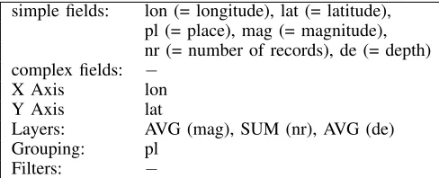
simple fields: lon (= longitude), lat (= latitude), pl (= place), mag (= magnitude), nr (= number of records), de (= depth) complex fields: −

X Axis lon

Y Axis lat

Layers: AVG (mag), SUM (nr), AVG (de)

Grouping: pl

Filters: −

Fig. 3. The data specification for the visualization of Fig. 1(b).

As an example of a data specification, consider again the visualization in Fig. 1(b). In this data specification, X corre-sponds to longitude, Yto latitude, and there are three layers: AVG(magnitude), SUM(number of records) and AVG(depth). We also need to mention that the data are being grouped by the value of “place.” (The attribute “place” is a usual construct included in geographical data sets; it is used to group the data points by their geographical location.) The full data specification for Fig. 1(b) is shown in Fig. 3.

Formally, a data specification is a tuple (X, Y, Layers,

Filters, Grouping), where X and Y are the fields rendered respectively as the X and Y axis, Layers is the set of fields rendered as layers, Filters is the set of filters in use, and Grouping is the set of attributes being grouped. Continuing with our example, the data specification for Fig. 1(b) is

(lon, lat, { AVG (mag), SUM (nr), AVG (de) }, pl, - ).

Intuitively, a data specification is a template for a SQL query of the form3

SELECT <fields to be displayed> FROM <data set>

WHERE <filters on nonaggregated fields>

GROUP BY <grouping specification, X and Y axis> HAVING <filters on aggregated fields>

The connection between data specifications and SQL is important, as it provides flexibility when communicating with the log of visualization systems: We can either capture their data specifications, or we can capture SQL queries and produce specifications ourselves. For our example, the query is

SELECT Latitude, Longitude, AVG(magnitude), SUM(number of records), AVG(depth) FROM Earthquakes

WHERE Latitude < 49.5 AND Latitude > 5.3 AND Longitude < -24.5 AND Longitude > -128.7 GROUP BY Place

(Sometimes we may need the visual specification to generate the SQL query for a given data specification. For example, in this case we have restricted the Latitude and the Longitude, but this information is stored in the visual specification.)

The Navigation Algebra:We now specify operations on data specifications. The purpose is to enable transitions from one data specification to the next in a visual-exploration sequence that a user generates on the data. The basic operations for transforming data specifications are as follows:

• Add or remove a filter condition;

• Add or remove a field to/from the SELECTcondition (that is, the fields rendered as a layer),X axis, orY axis;

3_{This is the way specifications are generated in, e.g., the Polaris prototype}

• Add or remove a field to/from grouping specification; and

• Modify the specification of a complex field by adding or removing an operation (such as ×or +).

(In most systems, one can directly replace a field Awith a fieldB.For technical reasons, we choose to model this action with two operations: removing Aand then adding B.)

We use the Navigation Algebra to represent how users navi-gate between visualization in a step-by-step fashion. Consider, for example, a user going from the visualization of Fig. 1(b) to that of Fig. 1(c). We can model this as a sequence of three data specifications, starting with

(lon, lat, { AVG (mag), SUM (nr), AVG (de) }, pl, - ),

then removing depth, to obtain

(lon, lat, { AVG (mag), SUM (nr) }, pl, - ),

and then removing the number of records, to arrive at

(lon, lat, { AVG (mag) }, pl, - ),

which corresponds to the data specification of Fig. 1(c). Sequences and Data-Slice Graphs: When working on a visual-exploration or visual-analysis task, users create what we call sequences of visualizations: Starting at a particular visualization (such as that of Fig. 1(b)), a user can create new visualizations (such as the one of Fig. 2(a)), by performing operations made available to them by the user interface – e.g., filtering the data, adding an extra attribute to the data specifi-cation, or changing the type of visualization. Each subsequent operation produces a new visualization in the sequence, and users continue in this fashion until completion of their task.

Our goal is to suggest to the user the slice of the data whose visualization is appropriate for the current stage of the user’s task on the data. Thus, we do not concentrate on those parts of the sequences where new visualizations are created by modifying the visual specification. Rather, we focus on the underlying sequence given by the changes in the data specifications. These changes are modeled using our Navigation Algebra as described above. Assuming that we have a log with visualization sequences generated by previous users, we construct what we call the Data-Slice Graph of this log: The nodes of this graph consist of all the data specifications occurring in the sequences in the log, and there is a directed edge from nodeD1to nodeD2if the log contains a

sequence whereD1andD2are consecutive data specifications.

As an example, Fig. 4(a) shows a data-slice graph for the task of finding outlier earthquakes in the data set [4] (Section I); this is task 1 in Section VII. The graph contains sequences generated by users who were solving the same type of task on the data set. Fig. 4(b) depicts a fragment of the graph, showing nodes with IDs14,13,8,9,23and24. Fig. 4(b) was generated by the user sequence(D8,D9,D23,D24,D23,D8,D13,D14).

That is, the user started in node 8, with the specification

D8 = ( longitude, latitude, {}, place, - ),

that is, assigning the earthquake longitude to the X axis, the latitude to theYaxis, and grouping byPlace. This specification corresponds to a visualization showing the map and just one dot for each place in that map where there has been at least one earthquake. (The grouping inD8means that all the earthquake

events in the same vicinity are grouped into a single tuple.) The user then went on to add a filter on the attribute Magnitude,

to filter out places where the average magnitude is not high enough. Note that rather than storing the precise filter, D8

stores just the fact that a filter was added. This allows us to store together all the data specifications with similar filters.

Continuing with the sequence, the user then added depth (node ID23with data specificationD23) and minimum depth

(24andD24), then removed the minimum depth to arrive back

at node 23. After this, the depth was removed (back to node 8), then the number of records was added (node13). Finally, the user removed the grouping clause (node 14), probably to see the entire data set at the same time.

Interesting Nodes:Some of the sequences of visualizations in a log may contain data that are important for the task assigned to the user. We denote these as interesting visual-izations, and mark them as interesting nodes in our data-slice graph.4For example, in our experiments with task 1 of Section VII, the nodes with IDs 9 and23in Fig. 4(b) were the most interesting to the human subjects. Since the data specification

D9 represents visualizations that are similar to that of Fig.

2(c), this confirms the intuition that the visualization in Fig. 2(c) is amongst the most informative for this type of task.

We distinguish between two types of users: experts and regular users. (This distinction is discussed in more detail in Section V-B.) We say that there is an expert (directed) edge from node D1 to nodeD2 if the sequence generatingD1 and

D2 was generated by an expert, and there is auser (directed)

edge if it was generated by a regular user. In addition, for each edge of the form (D1, D2) we maintain with the edge

the number of sequences in the log in whichD2 followedD1.

B. Algorithms to Match and Rank Data Slices

The main focus of our framework is on servicing user requests to recommend the next task-relevant data slice and its appropriate visualization. To continue with our example, suppose that a user is exploring the earthquakes data set for magnitude outliers in Central America, and is currently looking at the visualization of Fig. 1(b). The data specification for Fig. 1(b), as discussed in Section IV-A, is

(lon, lat, { AVG (mag), SUM (nr), AVG (de) }, pl, - ).

When the user asks for a recommendation, the system needs to perform the following two operations:

1. The data specification currently being examined by the user needs to be matched to a (data-specification) node in the data-slice graph. The easy special case is the current data specification being already represented by a node in the data-slice graph. In general, we need to locate in the graph one or more nodes that are closest to the current data specification, in terms of operations of the Navigation Algebra of Section IV-A. In our example, the data specification of Fig. 1(b) does not exists in the data-slice graph of Fig. 4(a), so we need to match it to the “best-match” node in the graph. The closest matches would be the nodes with IDs 8 and23. Intuitively, each of8 and23is just three operations away from the specification of Fig. 1(b). Indeed, to reach node 8 from Fig. 1(b), one needs to remove all three layers, and to reach node 23, we remove

4_{In general, determining whether a visualization is interesting to a user}

1 2 15 19 20 21 11 12 17 16 18 X Y Y X X X

(dmin, (p,t), . .) (dmin, p, . .)

(mag, p, . .)

(d, p, . .) (. (p,t), . .)

(.p, . .)

X

(. (d,dmin), p, .)

(. d, p, .)

Y

(n, p, . .) (t, . p, .) (. n, p, .)

Y,grp (. .p, .)

Y

X

Y 10

X, grp

(lon, . . .)

X,Y

3 4 5

13 7 23 6 8 9 14 22 24 (. (p,dmin), . .)

grp

grp Y

Y,grp Y

(. m, p, .) (. m, . .)

(. lat, . .) (lon, lat, p, .)

(lon, lat, p, m) (lon, lat, (p,d), m) (lon, lat, (d,dmin), m)

(lon, lat, p, n) (lon, lat, . .)

(lon, lat, . n)

Y grp grp fltr grp fltr grp grp, fltr fltr

An expert graph, each node defines (x, y, grouping, filter) values: d ≡ depth, dmin ≡ minimum depth,

lat ≡ latitutde, lon ≡ longitude, m ≡ magnitude, n ≡ number of records, p ≡ place, t ≡ time, . ≡ no value; each edge defines value transitions between two nodes: X ≡ x, Y ≡ y, grp ≡ grouping, fltr ≡ filter

(a) 1 2 15 19 20 21 11 12 17 16 18 X Y Y X X X

(d_min, (p,t), . .) (d_min, p, . .) (mag, p, . .)

(d, p, . .)

(. (p,t), . .)

(.p, . .)

X

(. (d,d_min), p, .)

(. d, p, .)

Y

(n, p, . .) (t, . p, .) (. n, p, .)

Y,grp (. .p, .)

Y

X

Y ₁₀

X, grp

(lon, . . .)

X,Y

3 4 5

13 7 23 6 8 9 14 22 24 (. (p,d_min), . .)

grp

grp Y

Y,grp Y

(. m, p, .) (. m, . .)

(. lat, . .)

(lon, lat, p, .)

(lon, lat, p, m) (lon, lat, (p,d), m)

(lon, lat, (d,dmin), m)

(lon, lat, p, n) (lon, lat, . .)

(lon, lat, . n)

Y grp grp fltr grp fltr grp grp, fltr fltr

An expert graph, each node defines (

x

,

y

,

grouping

,

filter

) values:

d

≡ depth,

d

≡ minimum depth,

lat

≡ latitutde,

lon

≡ longitude,

m

≡ magnitude,

n

≡ number of records,

p

≡ place,

t

≡ time, . ≡ no

value; each edge defines value transitions between two nodes:

X

≡

x

,

Y

≡

y

,

grp

≡

grouping

,

fltr

≡

filter

(b)

Fig. 4. (a) A data-slice graph for experimental Task 1 of Section VII. Each graph node is shown using its (x,y,grouping,f ilter) values, withd=depth,

dmin=minimum depth,lat=latitude,lon=longitude,m=magnitude,n=number of records,p=place,t=time, and .=no value. Edges define value

transitions between nodes, with X=x, Y=y, grp=grouping, fltr=f ilter. In (b), the bottom-right fragment of the graph is shown at higher resolution.

the magnitude and number of records, but introduce a filter on magnitude. We keep all such “best-match” nodes.

2. Once a match has been found, the system needs to find in the data-slice graph those “downstream” data specifications that are potentially interesting to the user and are at the same time the closest to the matched node, in terms of operations of the Navigation Algebra. In our example, this would correspond to nodes with IDs 9 and23.

The algorithm addressing the first challenge is called Match, please see Algorithm 1 for the pseudocode. The input of this algorithm is a data specification D, and we compute, for all nodes of the data-slice graph, the edit distance between

D and each of the specifications in the node of the stored data-slice graph G. (As mentioned in Section III, both this algorithm and the Rank Data Slice algorithm can use any distance measure, e.g., page rank. The edit distance shown in the pseudocode of Match is one specific choice made in our implementation described in Section VI.) We do not want to differentiate between the specifications where the X and the Y axis are switched, as they represent semantically the same object, and likewise for switching between layers and axis. Thus, we proceed as follows. For each node n in the graph we compute three distances between n and D: (1) The edit distance ds that considers only the fields assigned to the X andY axis and the layers inD andn; (2) the edit distancedg considering only the fields in the grouping clause; and (3) the edit distance df that considers only the filters in each of D andn. We then add the three values, and output all the nodes

n in the graph for which the resulting value is the lowest. We now look at addressing the second challenge listed above, making recommendations using the current match. Once we have matched a specification to a node in the data-slice graph, the next task is to retrieve the interesting “downstream” nodes in the graph that are the closest to the

matched node. We do this using our Rank Data Slices

algorithm, please see Algorithm 2 for the pseudocode. The algorithm works as follows. We assume that each nodekin the data-slice graph is given an “interestingness” value Ik. (Any interestingness measure will work for our purposes, as outlined in Section III.) We are also given a threshold T, with the objective of selecting only those nodes with an interestingness value above T, as well as the desired number M of output nodes. For each node n that is in the output of the Match function, we select all the nodes in the data-slice graph whose

interestingness value is greater than the thresholdT, and rank them in terms of their weighted-shortest-path distance to n. (Other distance measures could be used instead.) We then select and return the M nodes from this set that are closest ton; if there are not enough such nodes, we complete the list with the most interesting nodes overall according theI-values in the graph. (This might be necessary if, for instance, the user’s current visualization is not relevant to the task and thus cannot provide a useful input to the Matchalgorithm.)

Algorithm 1: Match Data Slices

Given: Data-slice graphGand maximal numberM of

nodes in the output.

Input: Data specificationD.

Output: The set of nodes of the data-slice graphGthat

is nearest to D in terms of edit distance.

foreach noden inGdo

ds=edit distance between the selection arguments of nandD;

da=edit distance between the filters ofn andD;

dg=edit distance between the grouping clauses of

nandD;

setdistance(n) =ds+da+dg;

returnup toM nodesninGwith the lowest values of

distance(n).

Algorithm 2: Rank Data Slices

Given: Data-slice graphG, maximal number of output

nodesM, interestingness value Ik for each nodek in

G, and interestingness thresholdT.

Input: A noden of the data-slice graphG.

Output: List ofM interesting nodes closest to n.

L=∅;

foreach nodem inGwithIm > T do compute

distance(m) =wheighted_shortest_path(n, m);

ifdistance(m)< inf initythen

add m to L;

SortL according to distance (ascending);

ifsize(L)>=M then

return theM first nodes ofL;

else

add toLthe M−size(L)most interesting nodes in

Gaccording toI that are not inL;

returnL.

V. CONSTRUCTING ANDUSINGDATA-SLICEGRAPHS

In this section we outline the process of constructing the data-slice graph for a given task type on a data set. Then we discuss the modes of using data-slice graphs depending on whether domain experts have been involved in the construction.

A. The Construction Algorithm

Recall (Section I) that we assume that each user declares her task as she begins the work. Thus, each user sequence can be associated in the log with the task that the user was solving when generating the sequence. We also assume that each expert sequence (if any) is marked as such by the log administrator; we discuss the implications later in this section. At the point of logging a completed user sequence, we reformulate it, with two goals in mind. First, we make sure that all the logged sequences are formulated “at the same level of granularity.” Toward this goal, we make each sequence detailed enough so that each edge in the output sequence corresponds to a single operation in the Navigation Algebra of Section IV-B (see Fig. 4(a) for an illustration of the outcome). The second goal is to mark, in each sequence, each node that is interesting under the given interestingness measure, see Sections III-B through IV-B for a discussion. The overall algorithm for this reformulation

of user sequences is straightforward.

Suppose now that we have selected from the log all the sequences that are to be included in the data-slice graph that we are constructing. (We discuss potential selection criteria in Section V-B.) We begin the construction by declaring one arbitrary selected sequence as the (initial) data-slice graph. We then keep adding all the other selected sequences to the graph one at a time, by combining each node in the current sequence with some node in the graph, as long as the two nodes are the same in the D part of theirVis=hD, Sirepresentation. That is, we combine a node in a user sequence with a node in the graph if and only if theDparts of these nodes are the same; we store with each resulting node as many visual (S) specifications as we had in all the nodes that we have combined. If, on the other hand, for a node n in the sequence being added there are no nodes in the data-slice graph that have the sameDpart as n, we just add n as a new node in the graph. For each node we keep the maximum interestingness amongst all the sequences in which this node appeared. Once we have merged all the nodes of a sequence with the graph in this manner, we add to the graph all the edges belonging to the sequence being added. In the process, if the sequence being added is an expert sequence, we re-weigh all its edges as described in the discussion of the Rank Data Slices algorithm in Section IV-B. Output and Correctness: The output of the overall graph-construction algorithm is a data-slice graph constructed as described above. By definition of the algorithm, its output does not depend on the order in which the selected input sequences are processed and merged with the graph. The construction can be done either in the batch fashion or with the graph being enhanced over time in an incremental fashion, with addition of one user sequence at a time as needed.

B. Recommendation and Prediction Systems

We are now ready to discuss possible criteria for selecting logged user sequences for entry into the data-slice graph.

Recommendation Systems:One criterion could be to include all the sequences from the log that are associated with the task type of interest. (Recall that we consider two tasks on the same data set to be the same if they only differ in the filtering criteria. E.g., we declare to be the same the tasks “find all the magnitude-outlier earthquakes in the world” and “find all the magnitude-outlier earthquakes in Central America” on the data set [4], see Section III-A.) In this case, there is no need to mark user sequences as expert, and thus the entire process of constructing both the log and the data-slice graph as described in Section V-A can be fully automatic.

Front End (Any Visualization Software)

User Asks Recommendation

Log Parser Construct Visual _Spec.

Data-Slice

Graph Match Function

Ranking Graph

Construction

Suggesting Helpful Visualization

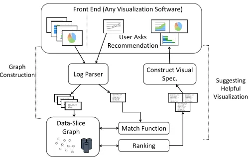
Fig. 5. The DataSlicer system architecture.

help of domain experts is available, or perhaps even sought after, as would be in case of mission-critical applications. Re-call that the log administrator can mark some of the sequences to be logged as coming from domain experts. This can be done in case one or more experts on the domain, task type, and data set are involved in solving tasks of this type for the benefit of the user community; the community could be employees of a certain company, analysts using a certain product, and so on. In this case, the process of constructing the graph is the same as before (see Section V-A), with expert nodes and edges being marked explicitly as such in the construction.

When the DataSlicer system uses a data-slice graph con-structed using expert sequences, we refer to this mode of op-eration as “prediction mode,” and to the system as a “prediction system.” Indeed, domain experts are expected to know how to solve effectively and efficiently tasks of the given type on the data set, and nodes and edges generated in the graph by their solutions are expected to help the community in solving tasks of the same type more so than sequences created by regular users. Note how our algorithm of Section V-A incorporates into a data-slice graph and automatically reconciles potentially different approaches of multiple experts to solving the same task. As a result, the sequences coming from multiple experts get transformed into multiple solution paths in the graph.

VI. PUTTINGITALLTOGETHER

Fig. 5 depicts a high-level overview of the architecture of our system. In this section we explain it component by component, and then discuss the scalability and implementation.

Front End: The front end of the system can be any visu-alization tool, as long as this tool can issue appropriate data-specification queries on the data-set store and visualize the answers, and also has a means of communicating its operations to other software. Some commercial visualization systems make available logs of their operations; we have implemented DataSlicer with a commercially available front-end tool, in such a way that all the communication with the front end is made through these logs, as explained in the next module.

Interface:The DataSlicer interface is the means to connect with the front-end visualization tool. The interface is in charge of the following two main tasks: First, we need a way of obtaining and understanding logs of the system, to be able to extract from the logs information about previous-user sessions. This part of the interface is called the log parser; it also maintains the current user’s current visual specification, as well

as the data specifications returned by the ranking algorithm of Section IV-B. Second, once the system has recommended a set of data specifications, these need to be visualized and presented back to the user. To create these visualizations, we maintain the current user’s previous visualization preferences and use them wherever possible to visualize the recommended data specifi-cations. For those recommended data specifications that cannot be visualized using the current user’s visual preferences, the system uses default visualization rules. Because of the closed architecture that many commercial visualization systems opt to implement, for our experiments we had to implement this second task in a semi-manual way.

Data-Slice Graph: The data-slice graph for the given task and data set is physically stored as a separate database. We do not, however, allow for any direct updates to the data-slice graph. Instead, to augment the data-slice graph with more information, we set up separate system sessions where past users sequences are provided to the log parser. During those sessions, the log parser enhances the existing data-slice graph with a new set of sequences, or creates a new data-slice graph from scratch, as detailed in Section V-A.

Back End:The back end of the system is the part that is in charge of producing recommendations for users. It comprises the Match and Rank algorithms, as described in Section IV-B. Scalability: In the DataSlicer architecture, visualizations are constructed for users by separate front-end visualization software, which sends to the data store queries based on the data slices, and then visually postprocesses the query answers. Thus, in the overall DataSlicer system, the processing of data-slice queries is decoupled from executing the Match and Rank algorithms of Section IV-B on the data-slice graphs. Further, data-slice graphs are constructed based on task-exploration sequences and thus on the structure rather than on the contents of the data set being explored. Thus, the size of each data-slice graph does not depend on the number of tuples of the data set, and does not need to be modified as the contents of the data set change over time. On the other hand, the size of a data-slice graph is directly proportional to the number of user sequences that it captures, and the Match and Rank algorithms clearly run in at most linear time with respect to the size of the graph. Addressing the issue of scalability of Match and Rank on data-slice graphs in the number of user sequences in the graph is a direction of our current work.

The Implementation: The system used for the experiments reported in Section VII has been built using the Java frame-work and compiled using JDK 1.8. To store the data-slice graphs for the experiments, we used MongoDB version 2.2. We worked with a commercial visualization tool; we can support working with any visualization tool, but for each different visualization tool, a different DataSlicer interface needs to be built. (This includes the log parser and the connection that presents visualizations back to the user.)

VII. EXPERIMENTALRESULTS

Name Position Age BA Melky Mesa UT 25 0.50 Derek Jeter SS 38 0.32 Andy Pettitte P 40 0.25 Francisco

Cervelli

C 26 0.00

Chris Dickerson

OF 30 0.29

Brett Gardner LF 28 0.32 Rabinson Cano 2B 29 0.31 Eric Chavez DH 34 0.28

(a) Fragment of data set [5] for task 2 (b) Box plot showing prominently answer outliers for task 2 on data set [5] Fig. 6. Experimental task 2 using data set [5]: fragment of the data set and a visual solution that shows prominently the answers to the task.

2005 2006 2007 2008 2009 2010

China 375 430 430 545 545 545

France 886 1148 1148 1248 1248 1248

Germany 765 765 765 887 937 937

Italy 1217 1217 1217 1231 1231 1245

Japan 957 957 957 957 957 970

Netherlands 1005 1005 1005 1020 942 942

United Kingdom

1267 1267 1267 1350 1160 1045

United States

1160 1160 1160 1245 1315 1315

(a) Import costs ($ / container) in 2005-2010 in [6] (b) Diagram showing prominently answers (trend outliers) for task 3 on data [6] Fig. 7. Experimental task 3 using data set [6]: fragment of the data set and a visual solution that shows prominently the answers to the task.

2000 2001 2002 2003

Export 279.56 299.41 365.40 485.00

Import 250.69 271.33 328.01 448.92

2004 2005 2006 2007

Export 655.83 836.90 1061.68 1342.21

Import 606.54 712.09 852.77 1034.73

2008 2009 2010

Export 1581.71 1333.30 1752.10

Import 1232.84 1113.20 1520.33

(a) Export and import values for China (top country in urban population) in billion US$ in 2000–2010 in data set [6]

(b) Line diagram showing prominently answer import/export trends for the top country in urban population in 2000-2010, for task 4 on data set [6]

Fig. 8. Experimental task 4 using data set [6]: fragment of the data set and a visual solution that shows prominently the answers to the task.

setup.) Following the experiments, each participant completed a questionnaire to capture their perception of: (1) the difficulty of the assigned task, (2) the correctness of their solution, (3) the correctness of the system’s solution, and (4) the overall usefulness of DataSlicer.

Both the statistical and questionnaire results were positive. Specifically, the results suggest that DataSlicer provides tech-nically correct visualizations and, perhaps more importantly, rapidly directs participants to a correct visualization, poten-tially improving their performance over time.

A. Procedure and Result Summary

We conducted four sets of experiments involving 48 human participants, with 12 participants randomly assigned to each of the four separate groups. The participants were graduate students ranging in age from 21 to 34, with 31 males and 17

females, each with normal or corrected to normal vision. Prior to the four sets of experiments, separate tests were conducted with four extra participants, to validate and debug both the DataSlicer software and the experimental procedure.

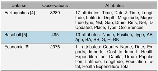
TABLE I. THE DATA SETS,NUMBER OF OBSERVATIONS,AND NUMBER AND NAMES OF ATTRIBUTES FOR THE FOUR EXPERIMENTAL TASKS.

Data set Observations Attributes

Earthquakes [4] 8289 17 attributes: Time, Date & Time, Longi-tude, LatiLongi-tude, Depth, MagniLongi-tude, Magni-tude type, Nst, Gap, Dmin, Rms, Net, ID, Updated, Place, Type, Occurrences Baseball [5] 495 10 attributes: Name, Position, Type, AB,

Age, BA, BB, G, H, RK

Economic [6] 2376 11 attributes: Country Name, Date, Ex-ports, ImEx-ports, Cost to Import, Health Expenditure per Capita, Urban Popula-tion, Latitude, Longitude, Population To-tal, Health Expenditure Total

by providing feedback via a questionnaire (see Section VII-E). The data sets used in the experiments are summarized in Table I, and the experimental results are given in Table II. Please note that the data sets (Table I) were small in size. Still, we found (Table II) that our human participants had difficulty completing the assigned tasks even on these small data sets. Presumably, increasing the number of observations would further degrade the users’ unassisted performance.

The analysis of the experimental results has identified sta-tistically significant improvements when access to DataSlicer was available, in terms of both accuracy and speed as defined in the beginning of this section. Welch’s analysis of variance (ANOVA) [30] confirmed that DataSlicer aided participants, helping them to perform tasks significantly faster and more accurately compared to a traditional visualization system (see Section VII-D). The tasks assigned to the participants include spatial outliers, local outliers, trend outliers, and general trends, which represent common analytic tasks on real data. Thus, the improved accuracy and speed in our experiments suggest better accuracy and speed for real-world data analysis.

B. The Tasks

Each participant was asked to perform one of the four dif-ferent tasks, both with and without assistance from DataSlicer: (1) locating spatial outliers in an earthquakes data set [4]; (2) locating data outliers in a baseball data set [5]; (3) locating outlier patterns and trends in an economic data set [6]; and (4) recognizing the general trends in the (same) data set [6]. The experiments were designed to cover common analytical tasks performed across a wide range of data domains; the tasks and data sets used in the experiments are as provided by [15].

The expert sequences for each task were generated and val-idated as part of the experimental setup. The experts’ log files were retrieved from the front-end visualization tool, parsed, and integrated into DataSlicer as discussed in Section V-A.

Task 1: Spatial Outliers.This task used an earthquakes data

set [4] containing the location of 8,289 earthquakes with mag-nitude 6 or greater throughout the world, from 1900 to 2013 (Table I). The participants were asked to findplaces(locations) on the map that contain earthquakes with either: (1) outlier magnitudes; or (2) outlier number of occurrences. Given the set of all outliers O, we define an outlier o ∈ O as a value that is more than 1.5 inter-quartile ranges IQR = Q3−Q1

above quartile boundary Q3 or below quartile boundary Q1,

o≥Q3+ 1.5IQR or o≤Q1−1.5IQR.

Task 2: Local Data Outliers. This task used a baseball data

set [5] containing 10 attributes for 45 baseball players from the 2012 Major League Baseball season (Table I). The participants

were asked to find the data points for players that were outliers based on a specificpositionortype. For example, a participant could look for outlier players at the shortstop position by identifying all shortstop players, then search for outliers within that subgroup. If a data point contained any attribute that was an outlier relative to the other players in the subgroup(hence the name “local data outliers”), then that player would be reported as an outlier.

Given the outlier sets for a given position or type for the 10 attributes O1, . . . , O10, we define an outlier oi ∈Oi as a value that is more than 1.5 inter-quartile ranges IQR_i above boundary Qi,1 or below boundaryQi,3,oi≥Qi,3+ 1.5IQRi or oi ≤Qi,1−1.5IQRi. If a player has at least one oi∀1≤

i≤10, that player is considered an outlier player.

Task 3: Outliers in Economic Patterns. This task used a

World Bank indicators data set [6] containing 11 economic, health, and population attributes for 216 countries for the years 2000–2010 (Table I). The participants were asked to identify the top eight countries in terms of average exports, then determine which of these countries displayed an outlier pattern in terms of exportstatistics over the given years. Outliers are identified by differences in the direction of the slope of their trend lines versus the overall norm for a given attribute.

Task 4: General Economic Patterns.This task used the same

data set [6] as Task 3. The participants were asked to identify a visualization that showed the similarities and dissimilarities between the export and import trends for the top country in the urban populationcategory over the years 2000 to 2010.

C. Expert Solutions

The following steps were used in the expert sequences (developed as part of the experimental setup) for each task.

Task 1. Identifying spatial outlier in the earthquakes data set

[4] involved two stages. First, the threshold needed to filter non-outlier observations is found using a box plot (Fig. 2(b)). The whiskers on the box plot define the exact upper and lower thresholds for outlier values ofmagnitudeor number of occurrences. Second, a map containing only the outlier values (Fig. 2(c)) is generated. Locations of outlier earthquakes on the map can then be identified.

Task 2. Similar to task 1, a boxplot is used to identify data

outliers in the baseball data set. First, players are nested within either position or type. This has the effect of focusing on a specific position or type. Next, boxplots for all ten attributes are generated to identify outlier thresholds for each attribute, for the given subgroup of players. Any player with an attribute value outside these thresholds, for any attribute, is considered an outlier player. Participants can hover over the sample points above or below the boxplot threshold whiskers to identify specific outlier players in the visualization (Fig. 6(b)).

Task 3. Identifyingexport pattern outliers in the World Bank

indicators data set [6] involved two stages. First, the top eight countries in terms of average exports were filtered by setting a lower export bound to include only eight countries. Next, a line graph visualization of each country’s exports over the years 2000 to 2010 was generated. The countries whose trend lines deviated in slope from the norm (i.e., the trend lines that did not follow the ascending or descending pattern of the norm) were deemed to be outliers (Fig. 7(b)).

Task 4. Recognizing general patterns in import and export

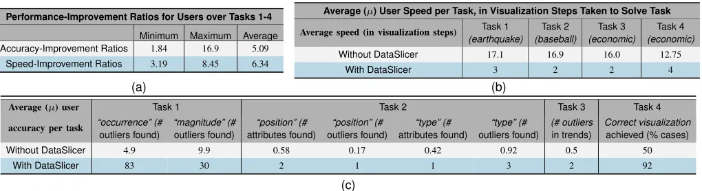
TABLE II. EXPERIMENTAL RESULTS: (A) PERFORMANCE IMPROVEMENTS,REPORTED FORACCURACY AS(WITHDATASLICER)/(WITHOUT

DATASLICER)RATIOS,AND FORSPEED AS(WITHOUTDATASLICER)/(WITHDATASLICER)RATIOS; (B) AVERAGE SPEED VALUES ACROSS THE TASKS; (C) AVERAGE ACCURACY VALUES ACROSS THE TASKS.

Performance-Improvement Ratios for Users over Tasks 1-4

Minimum Maximum Average Accuracy-Improvement Ratios 1.84 16.9 5.09

Speed-Improvement Ratios 3.19 8.45 6.34

Average (µ) User Speed per Task, in Visualization Steps Taken to Solve Task

Average speed (in visualization steps) Task 1

(earthquake)

Task 2

(baseball)

Task 3

(economic)

Task 4

(economic)

Without DataSlicer 17.1 16.9 16.0 12.75

With DataSlicer 3 2 2 4

(a) (b)

Average (µ) user Task 1 Task 2 Task 3 Task 4

accuracy per task “occurrence” (#

outliers found)

“magnitude” (#

outliers found)

“position” (#

attributes found)

“position” (#

outliers found)

“type” (#

attributes found)

“type” (#

outliers found)

(# outliers

in trends)

Correct visualization

achieved (% cases)

Without DataSlicer 4.9 9.9 0.58 0.17 0.42 0.92 0.5 50

With DataSlicer 83 30 2 1 1 3 2 92

(c)

indicators data set [6] involved two stages. First, the topurban population country in 2000–2010 was identified by setting a lower bound on urban population as a filter. Next, a line diagram was generated on imports and exports over these years. The resulting visualization contains the top country’s trends for both importsandexports(Fig. 8(b)).

D. Detailed Statistics for the Experimental Evaluation We used Welch’s analysis of variance (ANOVA) [30] to search for significant differences between the participant per-formance with and without assistance from DataSlicer. The results show that the participants were both faster5 and more accurate6_{with access to DataSlicer than without, withp-values} ranging from 0.009 to below 0.0001. Below we include a detailed report for each task.

Task 1. In task 1, the participants were asked to identify

locations that contain outlier earthquakes based on magni-tude and number of occurrences. For both attributes, the participants were more accurate, finding on average 9.9 out-liers without DataSlicer versus 30 outliers with DataSlicer for magnitude, and 4.9 versus 83 outliers on average for number of occurrences (F(1,11) = 57.85, p < 0.0001 and F(1,11) = 2966.98, p < 0.0001, respectively). The participants also required significantly fewer data-specification steps to complete the task with DataSlicer (3, on average) than without (17.08, on average). A comparison of the average number of data-specification steps combined over both tasks yielded F(1,11) = 98.06, p <0.0001.

Task 2. In task 2, the participants were asked to identify

players with outlier attribute values for a specific position or type. For both categories, the participants correctly identified more outlier players with DataSlicer than without (0.17versus 1 outlier on average, F(1,20.29) = 28.74, p < 0.0001 for position and0.92versus3outliers on average,F(1,12.06) = 26.62, p= 0.0002fortype). The participants also located more total attributes that contained outlier values using DataSlicer (0.58 versus 2 attributes found on average, F(1,13.87) = 29.96, p = 0.0001 for position and 0.42 versus 1 attribute found on average, F(1,17.28) = 28.74, p = 0.009 for type). Finally, the participants required fewer data-specification steps to report their results:16.91data-specification steps on average

5_{Increased speed here means that fewer data-specification operations were}

required with DataSlicer than without, to identify a correct visualization.

6_{Better accuracy here means that more outliers were located with DataSlicer}

than without, and general trends were located with DataSlicer but not without.

without DataSlicer, and 2 with DataSlicer, F(1,11.08) = 114.3, p <0.0001.

Task 3. In task 3, the participants were asked to identify

the top eight countries by average exports, then to determine which countries’ trend lines for each of the 11 attributes displayed outlier characteristics. The participants were able to correctly choose the top eight countries both with and without DataSlicer. However, the participants correctly located more outlier trend lines with DataSlicer (2, on average) than without (0.5, on average), F(1,13.22) = 26.71, p = 0.0002, and they were faster in terms of the number of data-specification steps required to identify the outliers (an average of 16 without DataSlicer versus 2 with DataSlicer), F(1,11.04) = 58.06, p <0.0001.

Task 4. In task 4, the participants were asked to construct

a visualization highlighting the similarities and dissimilarities between “export” and “import” trends for the top “urban population” country over the years 2000 to 2010. Twelve participants worked on task 4. Without DataSlicer, six of them were able to correctly obtain a final visualization, while the other six could not. With DataSlicer, the number of participants able to find a correct visualization increased to eleven, a sig-nificant improvement in accuracy (F(1,17.15)=5.85,p=0.0271). Moreover, the participants using DataSlicer accomplished the task more rapidly in terms of data-specification steps per-formed (an average of 12.75 without DataSlicer versus 4 with DataSlicer, F(1,13.56)=20.21, p=0.0006).

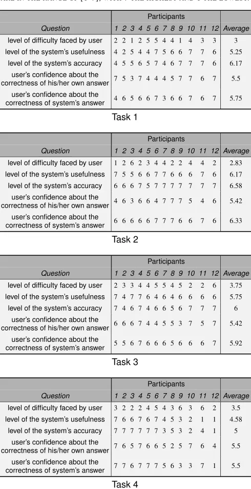
E. The User Questionaires

Table III shows the questions and answers, per task, in the questionnaires that we asked the human participants to com-plete for each experiment. (One questionnaire was comcom-pleted per participant per task.)

F. The Results