ELECTROCHEMICAL BEHAVIOUR OF PESTICIDES AT BARE AND NYLON 6,6-MODIFIED SOLID ELECTRODES IN DIFFERENTIAL PULSE
CATHODIC STRIPPING VOLTAMMETRY
THANALECHUMI A/P PARAMALINGGAM
ELECTROCHEMICAL BEHAVIOUR OF PESTICIDES AT BARE AND NYLON 6,6-MODIFIED SOLID ELECTRODES IN DIFFERENTIAL PULSE CATHODIC
STRIPPING VOLTAMMETRY
THANALECHUMI A/P PARAMALINGGAM
A thesis submitted in fulfilment of the requirements for the award of the degree of
Doctor of Philosophy (Chemistry)
Faculty of Science Universiti Teknologi Malaysia
I dedicate this thesis to my beloved family:
My dearest parents, Mr. Paramalinggam & Mrs. Thingalalaky
Jai Sri Maruthi
Om Namashivaya
Mr. Khartigesan & Mrs. Indrani
Mr. Thiyagarajan & Mrs. Gayathry
Mr. Gunalan & Mrs. Kalimah
Mr. Partiban & Mrs. Visalatshi
Sharenya
Reshikha
Thiran
Thebaan
Devesht
Shashinie
Tanissha & Taniskha
ACKNOWLEDGEMENT
First of all, I wish to give my highest praise to God “ellam pugallum iraivaneke” for showering me with love, blessings and strength to complete this Ph.D study.
My deepest gratitude goes to my supervisor Prof. Dr. Abdull Rahim Mohd. Yusoff for the continuous support of my Ph.D study and related research, for his patience, motivation and immense knowledge. His guidance assisted me in all the time of research and writing of this thesis. I could not imagine having such a great supervior for my Ph.D study.
I am also very thankful to all lecturers and lab assistants of the Department of Chemistry, Faculty of Science and Centre for Environmental Sustainability and Water Security (IPASA), Universiti Teknologi Malaysia, for their assistance and who gave access to the laboratory and research facilities. Without their precious support it would not be possible to conduct this research.
I also wish to thank Ministry of Higher Education Malaysia and Universiti Teknologi Malaysia for providing LRGS grant (R.J130000. 7809. 4L810) on Water Security entitled Protection of Drinking Water: Source Abstraction and Treatment (203/PKT/6720006) as financial support of this project. I am grateful for the UTM Zamalah scholarship and this support is greatly appreciated.
Finally, my sincere appreciation goes to my fellow labmates for the stimulating discussions, for the sleepless nights we were working together before deadlines, and for all the fun we had in the last four years.
To my beloved parents and all my family members, I would like to express my heartfelt gratitude for their love, motivation and supporting me spiritually in completing this overwhelming task.
ABSTRACT
ABSTRAK
Kajian tingkah laku voltammetri terhadap lima jenis racun perosak, iaitu parakuat diklorida, metsulfuron-metil, lindane, klorotalonil dan glifosat telah dijalankan. Elektrod yang telah digunakan ialah elektrod titisan merkuri (HMDE), elektrod karbon bak kaca (GCE), elektrod pensel HB (HBPE), elektrod berlian didopkan boron (BDDE), dan elektrod cetakan skrin (SPE). Disebabkan oleh ketoksikan merkuri dan untuk meningkatkan pengesanan bagi penentuan racun perosak, nilon-6,6 telah digunakan untuk mengubahsuai elektrod-elektrod tersebut untuk menghasilkan karbon bak kaca terubahsuai nilon-6,6 (Nyl-MGCE), elektrod pensel HB terubahsuai nilon-6,6 (Nyl-MHBPE), elektrod berlian didopkan boron terubahsuai 6,6 (Nyl-MBDDE) dan elektrod cetakan skrin terubahsuai nilon-6,6 (Nyl-MSPE). Semua pengukuran dijalankan dengan menggunakan teknik voltammetri pelucutan katod denyut pembezaan (DPCSV) vs. Ag/AgCl (3.0 M KCl). Parameter eksperimen misalnya pH penimbal Britton-Robinson (BRB), masa pengumpulan, potensi pengumpulan dan potensi awal telah dioptimumkan untuk penentuan racun perosak. Lakaran penentukuran linear bagi parakuat diklorida dan metsulfuron-metil diperoleh dengan nilai had pengesanan (LOD) masing-masing adalah 3.66 × 10⁻⁸ M dan 8.86 × 10⁻⁸ M pada HMDE. Pengesanan DPCSV dengan elektrod pepejal terubahsuai nilon-6,6 adalah lebih efektif berbanding dengan elektrod pepejal biasa, dengan nilai LOD untuk parakuat diklorida 2.75 × 10⁻⁸ M (GCE), 6.42 × 10⁻⁹ M (Nyl-MGCE), 2.37 × 10⁻⁸ M (HBPE), 1.33 × 10⁻⁸ M (Nyl-MHBPE), 2.52 × 10⁻⁸ M (SPE), 1.05 × 10⁻⁸ M (Nyl-MSPE), 2.86 × 10⁻⁸ M (BDDE)
dan 1.54 × 10⁻⁸ M (Nyl-MBDDE). Sensor baharu Nyl-MSPE dan Nyl-MHBPE telah digunakan untuk menganalisis lindane dan klorotalonil dengan LOD yang diperoleh masing-masing ialah 4.26 × 10⁻⁸ M dan 2.13 × 10⁻⁸ M. Usaha untuk mengkaji tingkah
TABLE OF CONTENTS
CHAPTER TITLE PAGE
DECLARATION ii
DEDICATION iii
ACKNOWLEDGEMENT iv
ABSTRACT v
ABSTRAK vi
TABLE OF CONTENTS vii
LIST OF TABLES xvi
LIST OF FIGURES xx
LIST OF ABBREVIATIONS xxxiv
LIST OF SYMBOLS xxxviii
LIST OF APPENDICES xl
1 INTRODUCTION 1
1.1 Background of Study 1
1.2 Problem Statement 4
1.3 Objectives of Study 5
1.4 Scope of the Study 6
1.5 Significance of Study 7
1.6 Thesis Outline 8
2 LITERATURE REVIEW 10
2.1 Agriculture in Malaysia 10
2.2 Pesticides and Their Importance 11
2.3 Impacts of Pesticides on Ecosystem 14
2.3.2 Reports Based on Regulation and Guidelines 16 2.4 Analytical Methods for Pesticide Determination 20
2.5 Electrochemical Techniques 21
2.5.1 Types of Voltammetric Techniques 23 2.5.1.1 Differential Pulse Voltammetry
(DPV)
23
2.5.1.2 Cyclic Voltammetry (CV) 23 2.5.1.3 Square-Wave Voltammetry (SWV) 24 2.5.1.4 Anodic Stripping Voltammetry
(ASV)
24
2.5.1.5 Cathodic Stripping Voltammetry (CSV)
25
2.5.1.6 Adsorptive Stripping Voltammetry (AdSV)
25
2.5.1.7 Linear Sweep Voltammetry (LSV) 26 2.6 Application of Voltammetry for Pesticide Analysis 27 2.7 Criteria for Selection of the Working Electrode Material 30 2.8 Polymeric Modification on Working Electrode 32
2.8.1 Types of Surface Modification 34
3 EXPERIMENTAL 37
3.1 Chemicals and Reagents 37
3.2 Voltammetry Instrumentation 38
3.2.1 Working Electrodes 39
3.3 Preparation of Nylon 6,6 Solution 40
3.4 Preparation of Stock Solutions 41
3.4.1 Paraquat Dichloride Standard Solution 41 3.4.2 Metsulfuron-Methyl Standard Solution 41
3.4.3 Lindane Standard Solution 42
3.4.4 Chlorothalonil Standard Solution 42
3.4.5 Glyphosate Standard Solution 42
3.4.6 Britton-Robinson Buffer 42
3.4.8 Hydrochloric Acid Solution 43
3.5 Preparation of Metal Solutions 43
3.5.1 Cadmium Standard Solution 44
3.5.2 Copper Standard Solution 44
3.5.3 Iron Standard Solution 44
3.5.4 Lead Standard Solution 44
3.5.5 Zinc Standard Solution 45
3.6 Voltammetry Procedures 45
3.6.1 Optimization of Voltammetric Operating
Parameters 45
3.6.1.1 Effect of pH of BRB 45
3.6.1.2 Effect of Initial Potential 46 3.6.1.3 Effect of Accumulation Potential 46 3.6.1.4 Effect of Accumulation Time 46
3.7 Calibration Curve 46
3.8 Interference Study 47
3.9 Pesticides Analysis in Water Samples 48
3.10 River Water Sampling 48
3.11 Characterization of Electrodes and Modifier 50
3.11.1 Morphological Analysis 50
3.12 Analytical Technique for UV-Vis Spectrophotometry Analysis
51
3.12.1 Analysis of Pesticides in Water Samples 51
4 DIFFERENTIAL PULSE CATHODIC STRIPPING
VOLTAMMETRIC DETERMINATION OF PARAQUAT DICHLORIDE AND METSULFURON-METHYL IN AQUEOUS SAMPLES USING HANGING MERCURY
DROP ELECTRODE 52
4.1 Introduction 52
4.2 Voltammetric Determination of Paraquat Dichloride on Hanging Mercury Drop Electrode Using Differential
4.2.1 Effect of Operating Parameter on Peak Current 53 4.2.1.1 Effect of pH for Paraquat Dichloride
Determination 53
4.2.1.2 Effects of Initial Potential, Accumulation Potential, Time Accumulation for Paraquat
Dichloride Analysis 57
4.2.2 Analytical Characteristics of Paraquat
Dichloride Using DPCSV Technique 59
4.2.3 Interference Study 60
4.2.4 Validation of the Proposed Method in Determination of Paraquat Dichloride in the
Commercial Paraquat 62
4.3 Voltammetric Determination of Metsulfuron-Methyl in
Water Samples Using DPCSV Technique 63
4.3.1 Effect of pH 64
4.3.2 Effects of Initial Potential, Accumulation Potential, Accumulation Time on
Metsulfuron-Methyl Analysis 65
4.3.3 Analytical Characteristics of
Metsulfuron-Methyl Using DPCSV Technique 67
4.3.4 Interference Study 69
4.3.5 Application of Proposed Method in Real Samples Analysis
71
4.4 Summary 72
5 SENSITIVE VOLTAMMETRIC METHODS FOR THE
DETERMINATION OF PARAQUAT DIHCLORIDE
USING NYLON 6,6 MODIFIED BORON-DOPED
DIAMOND AND GLASSY CARBON ELECTRODES 73
5.1 Introduction 73
6,6-Modified Boron-Doped Diamond Electrode 73
5.2.1 Effect of Modifier Dosage 74
5.2.1 Effect of pH 75
5.2.3 Optimization of Voltammetric Operating
Variables 78
5.2.4 Calibration Curve 80
5.2.5 Repeatability and Interference Study 82
5.2.6 Analysis on Real Samples 83
5.2.7 Morphological Studies 85
5.3 Effect of Voltammetric Parameters on the Determination of Paraquat at Bare and Nylon
6,6-Modified Glassy Carbon Electrode 86
5.3.1 Effect of Modifier Dosage 86
5.3.2 Effect of pH 87
5.3.3 Optimization of Voltammetric Operating
Variables 90
5.3.4 Analytical Procedure for Paraquat Dichloride
Quantification 93
5.3.5 Repeatability and Interference Study 95
5.3.6 Analysis on Real Samples 97
5.4 Comparison of Developed Sensors to UV-Vis
Spectrophotometry 98
6 ELECTROCHEMICAL BEHAVIOUR AND QUANTIFICATION OF THE PARAQUAT DICHLORIDE USING MODIFIED PENCIL LEAD AND SCREEN PRINTED ELECTRODES AS POTENTIAL SENSORS 6.1 Introduction
6.2 Screen Printed Electrode Modified With Nylon 6,6 As A Sensitive Voltammetric Sensor for Determination of Paraquat Dichloride
6.2.1 Effect of Experimental Parameters 6.2.1.1 Effect of Modifier Dosage 6.2.1.2 Effect of pH
6.2.1.3 Optimization of Voltammetric Operating Variables
6.2.2 Calibration Curve
6.2.3 Repeatability and Interference Study 6.2.4 Analysis on Real Samples
6.2.5 Morphological Studies
6.3 Effect of Voltammetric Parameters on Paraquat Dichloride Analysis using Bare and Nylon 6,6 Modified HB Pencil Lead
6.3.1 Effect of Modifier Dosage 6.3.2 pH Optimization
6.3.3 Optimization of Voltammetric Operating Variables
6.3.4 Analytical Procedure for Paraquat Dichloride Quantification
6.3.5 Interference Study
6.3.6 Analysis on Real Samples
6.4 Comparison of Developed Sensors to UV-Vis Spectrophotometry
6.5 Summary
7 VOLTAMMETRIC DETERMINATION OF CHLOROTHALONIL AND LINDANE USING GREEN SENSORS: GRAPHITE HB PENCIL AND SCREEN PRINTED ELECTRODES MODIFIED WITH NYLON 6,6 7.1 Introduction
7.2 Differential Pulse Cathodic Stripping Voltammetry of Lindane on Bare and Nylon 6,6 Modified Graphite HB Pencil Electrode
7.2.1 Effect of Experimental Parameters 7.2.1.1 Effect of Modifier Dosage 7.2.1.2 Effect of pH
7.2.1.3 Effect of Initial Potential, Accumulation Potential and Accumulation Time
7.2.2 Calibration Curve 7.2.3 Interference Study
7.2.4 Analysis on Real Samples
7.3 Differential Pulse Cathodic Stripping Voltammetry of Chlorothalonil on Bare and Nylon 6,6 Modified Graphite HB Pencil Electrode
7.3.1 Effects of Experimental Parameters 7.3.1.1 Effect of Modifier Dosage 7.3.1.2 Effect of pH
7.3.1.3 Effect of Initial Potential, Accumulation Potential and Accumulation Time 7.3.2 Calibration Curve
7.3.3 Interference Study 7.3.4 Real Samples Analysis
7.3.5 Comparison with Mercury Electrode
7.4 Voltammetric Determination of Lindane on Bare and Modified Screen Printed Electrode (SPE) Using Differential Pulse Cathodic Stripping Voltammetry (DPCSV)
7.4.1 Effects of Experimental Parameters
7.4.1.1 Effect of Modifier Dosage
7.4.1.2 Effect of pH of Supporting Electrolyte
7.4.1.3 Effect of Initial Potential, Accumulation Potential and Accumulation Time
7.4.2 Analytical Calibration Curve 7.4.3 Interference Study
7.4.4 Real Samples Analysis
7.5 Determination of Chlorothalonil on Bare and Modified Screen Printed Electrode (SPE) Using Differential Pulse Cathodic Stripping Voltammetry (DPCSV) 7.5.1 Effect of Experimental Parameters
7.5.1.1 Effect of Modifier Dosage 7.5.1.2 Effect of pH
7.5.1.3 Effect of Initial Potential, Accumulation Potential and Accumulation Time
7.5.2 Analytical Calibration Curve 7.5.3 Interference Study
7.5.4 Application of Developed SPE for the Determination of Chlorothalonil in Water Samples
7.6 Comparison of Developed Sensors to UV-Vis Spectrophotometry
7.7 Summary
8 CONCLUSIONS AND RECOMMENDATIONS 8.1 Conclusions
8.2 Recommendations
LIST OF TABLES
TABLE NO. TITLE PAGE
2.1 Pesticides and its functions 11
2.2 Common pesticides used in agriculture 12
2.3 World pesticide usage at the producer level by pesticide
type, 2011 and 2012 estimates 12
2.4 Classification of pesticides according to toxicity,
expressed as LD50 (mg/kg) 14
2.5 Long-term effects of pesticides on human health 16
2.6 Interim national water quality standard (INWQS) of
pesticides 17
2.7 Physical properties of the selected pesticides 19
2.8 Pesticides determination using different analytical
techniques 20
2.9 Voltammetric techniques applied for environmental
applications 27
2.10 Studies on pesticides using voltammetric techniques 28
2.11 A list of common conductive polymers 33
2.12 Conductivity values of some conductive polymers 33
2.13 Polymeric modification of working electrode for
pesticides analysis 35
3.1 Concentrations of nylon 6,6 solution 41
3.2 Concentrations of metal standard solutions 43
4.1 Parameters of the DPCSV calibration plot for paraquat
4.2 Recovery values of standard paraquat and commercial
paraquat dichloride 62
4.3 Recovery values for paraquat dichloride in spiked water
samples 63
4.4 Parameters of DPCSV calibration plot for
metsulfuron-methyl 68
4.5 Recovery values of metsulfuron-methyl in ultra-pure water (spiked) and in commercial product, Ally at
different level of concentrations 71
4.6 Real water samples analysis for metsulfuron-methyl 72
5.1 Optimization of nylon 6,6 dosage for BDDE
modification 74
5.2 Summary results of paraquat dichloride analysis using
DPCSV technique 81
5.3 Recovery values of paraquat dichloride in commercial
paraquat at different level of concentrations 84
5.4 Determination of paraquat dichloride in real water
samples 84
5.5 Optimization of nylon 6,6 dosage for GCE modification 87
5.6 The optimum parameters of paraquat dichloride
determination 91
5.7 Summary results of paraquat dichloride analysis at bare
GCE and Nyl-MGCE using DPCSV technique 94
5.8 Recovery values of paraquat dichloride in commercial
paraquat at different level of concentrations 97
5.9 Determination of paraquat dichloride in real water
samples 98
5.10 Summary results of paraquat dichloride analysis at bare BDDE, Nyl-MBDDE, bare GCE and Nyl-MGCE using
DPCSV technique 99
5.11 Comparison of various voltammetric studies for
5.12 Analysis on paraquat dichloride in tap and river water
samples using DPCSV and UV-vis spectrophotometry 100
6.1 Optimization of Nylon 6,6 dosage for SPE modification 103
6.2 The optimum parameters of paraquat dichloride
determination 108
6.3 Comparison of LOD value for paraquat dichloride
determination 110
6.4 Recovery values of paraquat dichloride in commercial
paraquat at different level of concentrations 113
6.5 Determination of paraquat dichloride in real water
samples 113
6.6 Optimization of nylon 6,6 dosage for HBPE
modification 117
6.7 Summary results of paraquat dichloride analysis at bare
HBPE and Nyl-MHBPE using DPCSV technique 122
6.8 Determination of paraquat dichloride in real water
samples 124
6.9 Comparison of LOD values for paraquat dichloride
determination 125
6.10 Analysis on paraquat dichloride in tap and river water
samples using DPCSV and UV-vis spectrophotometry 125
7.1 Optimization of nylon 6,6 dosage for HBPE
modification 129
7.2 Summary on optimization results for lindane analysis 134
7.3 Summary results of lindane using DPCSV 136
7.4 Determination of lindane in water sample using bare
HBPE 140
7.5 Determination of lindane in water samples using
Nyl-MHBPE 140
7.6 Optimization of nylon 6,6 dosage for HBPE
modification 142
7.8 Comparison on LOD values of chlorothalonil with other
published studies 149
7.9 Determination of chlorothalonil in real water samples
using bare HBPE 151
7.10 Determination of chlorothalonil in water samples using
Nyl- MHBPE 151
7.11 Optimization of nylon 6,6 dosage for SPE modification 154
7.12 Summary results of lindane at bare SPE and Nyl-MSPE
using DPCSV 161
7.13 Determination of lindane at bare SPE in real water
samples using DPCSV method 164
7.14 Determination of lindane at Nyl-MSPE in real water
samples using DPCSV method 164
7.15 Optimization of nylon 6,6 dosage for SPE modification 166
7.16 Summary on optimization results for chlorothalonil
analysis 171
7.17 Summary results of chlorothalonil at bare SPE and
Nyl-MSPE using DPCSV 173
7.18 Determination of chlorothalonil at bare SPE in real
water samples using DPCSV method 176
7.19 Determination of chlorothalonil at Nyl-MSPE in real
water samples using DPCSV method 176
7.20 Summary results of lindane analysis using DPCSV and
UV-vis spectrophotometry 177
7.21 Summary results of chlorothalonil analysis using
DPCSV and UV-vis spectrophotometry 178
7.22 Water samples analysis of lindane using UV-vis
spectrophotometry 179
7.23 Water samples analysis of chlorothalonil using UV-vis
LIST OF FIGURES
FIGURE NO. TITLE PAGE
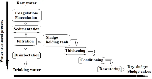
1.1 Water treatment processes 1
2.1 Classification of pesticides by chemical structure 13
2.2 Effects of pesticides on ecosystem 15
2.3 Chemical structures of the selected pesticides 18
2.4 Voltammetry electrodes system 22
2.5 Electrodes used in voltammetry analysis 22
2.6 Potential window range for some common working
electrodes 31
2.7 Dip-coating process 36
3.1 Voltammetry PGSTAT 30 Autolab Metrohm Model
and VA 663 stand 38
3.2 Voltammetric cell with three electrodes system 39
3.3 Working electrodes (a) HMDE, (b) SPE, (c) HBPE,
(d) BDDE and (e) GCE 40
3.4 HB pencil lead modification 40
3.5 Photographic view of the river water sampling
location 49
3.6 Location of water sampling point (red spot): From (A) (UTM) to (B) Kampung Jaya Sepakat (nearer to
sampling point) 49
4.1 Effect of pH on DPCSV peak current of 1.5×10‒6 M paraquat dichloride.The experimental conditions were as follows: Ei = 0 V, Ef = −1.2 V, tacc= 30 s, ʋ=
20 mV s‒1 and pulse amplitude = −50 mV 54
4.2 (A) Plot peak potential vs. pH and (B) DPCS voltammogram of 1.5×10‒6 M paraquat dichloride at different pH BRB. The experimental conditions were as follows: Ei = 0 V, Ef = −1.2 V, tacc = 30 s, ʋ=
20 mV s‒1 and pulse amplitude = −50 mV 55
4.3 DPCS voltammogram of paraquat dichloride at pH 2.0 of 0.04 M BRB. Concentration of analyte: (a) 0, (b) 0.5×10‒6 M, (c) 1.5×10‒6 M, and (d) 2.5×10‒6 M. The experimental conditions were as follows: Ei= 0
V, Ef= −1.2 V, tacc= 30 s, ʋ= 20 mV s‒1 and pulse
amplitude = −50 mV 56
4.4 Optimization of operating parameters for 1.5×10‒6 M paraquat dichloride determination using HMDE: (A) Ei, (B) Eacc and (C) tacc. The experimental conditions
were as follows: pH 2.0 of 0.04 M BRB, ʋ= 20 mV
s−1 and pulse amplitude = −50 mV 58
4.5 (A) DPCS voltammogram corresponding to the calibration curve of paraquat dichloride with concentrations: (a) 0, (b) 2.5×10⁻⁷ M, (c) 5.0×10⁻⁷ M, (d) 7.5×10⁻⁷ M, (e) 1.0×10⁻⁶ M, (f) 1.25×10⁻⁶ M, (g) 1.5×10⁻⁶ M, and (h) 1.75×10⁻⁶ M and (B) Calibration plot for DPCSV of paraquat dichloride. The experimental conditions were as follows: pH 2.0 of 0.04 M BRB, Ei= −0.6 V, Ef= −0.7 V, tacc= 30 s,
ʋ= 20 mV s‒1 and pulse amplitude = −50 mV 59
4.6 DPCS voltammogram of paraquat dichloride with increasing concentration: (a) 0, (b) 0.5×10⁻⁶ M, (c) 1.5×10⁻⁶ M, and (d) 2.5×10⁻⁶ M at pH 2.0 of 0.04 M BRB. The experimental conditions were as follows: Ei= −0.6 V, Ef= −0.7 V, tacc= 30 s, ʋ= 20 mV s‒1 and
pulse amplitude = −50 mV 60
4.7 (A) DPCS voltammogram of paraquat dichloride after the addition of Cd2+ ion (B) Effect of Cd2+ ion on peak current and (C) The effects of metal ion concentrations on Ip of paraquat dichloride. The
experimental conditions were as follows: pH 2.0 of 0.04 M BRB, Ei= −0.6 V, Ef= −0.7 V, tacc= 30 s, ʋ=
4.8 DPCS voltammogram of 2.5×10‒6 M of metsulfuron-methyl in 0.04 M BRB at pH (a) pH 2.0, (b) pH 3.0 and (c) pH 4.0. The experimental conditions were as follows: Ei = 0 V, Ef = −1.2 V,
tacc = 30 s, ʋ= 20 mV s‒1, pulse amplitude = −50 mV 64
4.9 DPCS voltammogram of metsulfuron-methyl as a function of concentration in pH 2.0 of 0.04 M BRB. Concentration of analyte: (a) 0, (b) 0.5×10‒6 M, (c) 1.5×10‒6 M, and (d) 2.5×10‒6 M. The experimental conditions were as follows: Ei= 0 V, Ef= −1.2 V,
tacc= 30 s, ʋ= 20 mV s‒1 and pulse amplitude = −50
mV
65
4.10 Optimization of operating parameters for 1.5×10‒6 M metsulfuron-methyl determination using HMDE: (A) Ei, (B) Eacc and (C) tacc. The experimental
conditions were as follows: pH 2.0 of 0.04 M BRB,
ʋ= 20 mV s‒1 and pulse amplitude = −50 mV 67
4.11 (A) DPCS voltammogram corresponding to the calibration curve of metsulfuron-methyl with concentrations: (a) 0, (b) 2.5×10‒7 M, (c) 5.0×10‒7 M, (d) 7.5×10‒7 M, (e) 1.0×10‒6 M, (f) 1.25×10‒6 M, (g) 1.5×10‒6 M, (h) 1.75×10‒6 M, and (i) 2.00×10‒6 and (B) Calibration plot for DPCSV of metsulfuron-methyl. The experimental conditions were as follows: pH 2.0 of 0.04 M BRB, Ei= −0.5 V, Ef=
−0.5 V, tacc= 60 s, ʋ= 20 mV s‒1 and pulse amplitude
= −50 mV 68
4.12 DPCSV voltammogram of metsulfuron-methyl with increasing concentration: (a) 0, (b) 0.5×10‒6 M, (c) 1.5×10‒6 M, and (d) 2.5×10‒6 M in pH 2.0 of 0.04 M BRB. The experimental conditions were as follows: Ei= −0.5 V, Ef= −0.5 V, tacc= 60 s ʋ= 20 mV s‒1 and
pulse amplitude = −50 mV 69
4.13 (A) DPCS voltammogram of metsulfuron-methyl with increasing concentration of Pb2+ ion (B) Effect of Pb2+ion on I
p and (C) The effects of metal ion
concentrations on Ip of metsulfuron-methyl. The
experimental conditions were as follows: pH 2.0 of 0.04 M BRB, Ei= −0.5 V, Ef= −0.5 V, tacc= 60 s, ʋ=
5.1 DPCS voltammogram of 2.5×10⁻⁵ M paraquat dichloride at different pH of 0.04 M BRB: (A) bare BDDE and (B) Nyl-MBDDE. The experimental conditions were as follows: Ei = 0 V, Ef = –1.4 V,
Eacc = 0 V, tacc = 30 s, ʋ = 20 mV s–1 and pulse
amplitude = –50 mV 76
5.2 Plot of peak current vs. pH for 2.5×10⁻⁵ M paraquat dichloride at bare and Nyl-MBDDE. The experimental conditions were as follows: Ei= 0 V,
Ef= −1.4 V, Eacc= 0 V, tacc = 30 s, ʋ= 20 mV s–1 and
pulse amplitude = −50 mV 77
5.3 DPCS voltammogram of paraquat dichloride at optimum pH 10.0 of 0.04 M BRB: (A) bare BDDE and (B) Nyl-MBDDE: (a) 0, (b) 0.5×10⁻⁵ M, (c) 1.5×10⁻⁵ M, (d) 2.5×10⁻⁵ M. The experimental conditions were as follows: Ei = 0 V, Ef = −1.4 V,
Eacc = 0 V, tacc = 30 s, ʋ= 20 mV s–1 and pulse
amplitude = −50 mV 77
5.4 Effect of voltammetric operating variables on peak current at 2.5×10⁻⁶ M of paraquat dichloride at optimum pH 10.0 of BRB. (A) Ei, (B) Eacc, and (C)
tacc. The experimental conditions were as follows:
Ef= −1.4 V, ʋ= 20 mV s–1 and pulse amplitude= −50
mV
79
5.5 DPCS voltammogram of 2.5×10⁻⁶ M paraquat dichloride at optimum pH 10.0 of BRB: (A) Nyl-MBDDE and (B) bare BDDE: The experimental conditions were as follows: Ei= −0.3 V, Ef = −1.4 V,
Eacc= −0.4 V, tacc = 30 s, ʋ= 20 mV s–1 and pulse
amplitude = −50 mV 80
5.6 Calibration curves and calibration plots for DPCSV of (A) bare BDDE and (B) Nyl-MBDDE: (a) 0 (b) 2.0×10⁻⁷ M, (c) 3.0×10⁻⁷ M, (d) 4.0×10⁻⁷ M, (e) 5.0×10⁻⁷ M, (f) 6.0×10⁻⁷ M and (g) 7.0×10⁻⁷ M. The experimental conditions were as follows: Ei= −0.3
V, Ef= −1.4 V, Eacc= −0.4 V, tacc= 30 s, ʋ= 20 mV s–1
and pulse amplitude= −50 mV 81
5.7 Graph peak current of paraquat dichloride vs. added concentration of metal ions. (A) bare BDDE and (B) Nyl-MBDDE. The experimental conditions were as follows: Ei= −0.3 V, Ef= −1.4 V, Eacc= −0.4 V, tacc=
5.8 DPCSV voltammogram of paraquat dichloride (A) bare BDDE and (B) Nyl-MBDDE with increasing concentration of Cu2+ ion (a) pH 10.0 of 0.04 M BRB (b) 2.5×10⁻⁶ M paraquat dichloride (c) 0.1 ppm Cu2+ ion, (d) 0.3 ppm Cu2+ ion and (e) 0.5 ppm Cu2+ ion. The experimental conditions were as follows: Ei= ̶ 0.3 V, Ef= ̶ 1.4 V, Eacc= ̶ 0.4 V, tacc = 30 s, ʋ=
20 mV s–1 and pulse amplitude= ̶ 50 mV 83
5.9 SEM micrographs of (A) bare BDDE and (B)
Nyl-MBDDE 85
5.10 DPCS voltammograms of 2.5×10 ̶ 5 M of paraquat dichloride at different pH BRB: (A) GCE and (B) Nyl- MGCE. The experimental conditions were as follows: Ei = 0 V, Ef = −1.4 V, Eacc = 0 V, tacc = 30 s,
ʋ = 20 mV s–1
and pulse amplitude = −50 mV 88
5.11 Plot of peak current vs. pH for 2.5×10 ̶ 5 Mparaquat dichloride at bare GCE and Nyl-MGCE. The experimental conditions were as follows: Ei= 0 V, Ef
= −1.4 V, Eacc = 0 V, tacc = 30 s, ʋ = 20 mV s–1 and
pulse amplitude = −50 mV 89
5.12 DPCS voltammograms of paraquat dichloride at (A) bare GCE (at pH 11.0 BRB) and (B) Nyl-MGCE (at pH 10.0 BRB) with the increasing concentrations (a) 0, (b) 0.5×10 ̶ 5 M, (c) 1.5×10 ̶ 5 M, (d)2.5×10 ̶ 5 M. The experimental conditions were as follows: pH BRB 11.0, Ei= 0 V, Ef= −1.4 V, Eacc= 0 V, tacc= 30 s,
ʋ = 20 mV s–1 and pulse amplitude = −50 mV 90
5.13 Optimization of operating parameters for 2.5×10⁻⁶ M paraquat dichloride determination using bare GCE (pH 11.0 of 0.04 M BRB) and Nyl-MGCE (pH10.0 of 0.04 M BRB): (A) Ei, (B) Eacc, and (C)
tacc. The experimental conditions were as follows:
Ef= −1.4 V, ʋ = 20 mV s–1 and pulse amplitude= −50
mV 92
5.14 DPCS voltammogram for 2.5×10⁻⁶ M paraquat dichloride at (a) bare GCE and (b) Nyl-MGCE at
optimum conditions as listed in Table 5.6 93
5.15 Calibration curves and calibation plots for 2.5×10⁻⁶ M paraquat dichloride using (A) bare GCE and (B) Nyl-MGCE. The experimental conditions were as in Table 5.6
5.16 Effects of metal ions on the peak current of 2.5×10⁻⁵ M paraquat dichloride at bare GCE in BRB 0.04 M at pH 11.0. The experimental conditions were as in
Table 5.6 95
5.17 Effects of metal ions on the peak current of 2.5×10⁻⁵ M paraquat dichloride at Nyl-MGCE in BRB 0.04 M at pH 10.0. The experimental conditions were as
in Table 5.6 96
5.18 Calibration plots for paraquat dichloride using
UV-vis spectrophotometry 99
6.1 Effects of pH on 2.5×10⁻⁵ M paraquat dichloride analysis at Nyl-MSPE: (A) DPCS voltammogram, (B) Peak current vs. pH and (C) Peak potential vs. pH. The experimental conditions were as follows: Ei= 0 V, Ef= –1.2 V, Eacc= 0 V, tacc= 30 s, ʋ= 20 mV
s–1 and pulse amplitude = –50 mV 105
6.2 DPCS voltammogram of paraquat dichloride: (A) bare SPE (optimal pH 10.0) and (B) Nyl-MSPE (optimal pH 9.0): (a) 0, (b) 0.5×10⁻⁵ M, (c) 1.5×10⁻⁵ M, (d) 2.5×10⁻⁵ M. The experimental conditions were as follows: Ei= 0 V, Ef= –1.4 V, Eacc= 0 V,
tacc= 30 s, ʋ= 20 mV s–1 and pulse amplitude = –50
mV
106
6.3 Effect of optimization parameters: (A) Ei, (B) Eacc
and (C) tacc at bare and modified SPE. The
experimental conditions were as follows: Ef = –1.4
V, ʋ= 20 mV s–1 and pulse amplitude = –50 mV 107
6.4 DPCS voltammogram for 2.5×10⁻⁶ M paraquat dichloride at (a) bare SPE and (b) Nyl-MSPE at
optimum conditions as listed in Table 6.2 108
6.5 Calibration curves and calibration plots for DPCSV of (A) bare SPE and (B) Nyl-MSPE at optimum conditions (a) 0, (b) 1×10⁻⁷ M (c) 2×10⁻⁷ M, (d) 3×10⁻⁷ M, (e) 4×10⁻⁷ M, (f) 5×10⁻⁷ M and (g) 6×10⁻⁷
M. The experimental conditions were as in Table 6.2 109
6.6 (A) DPCS voltammogram of 2.5×10⁻⁶ M paraquat dichloride analysis using bare SPE with the addition of Pb2+ ion, (B) Graph peak current of paraquat dichloride vs. added concentration of Pb2+ ion and (C) Interference studies of other metal ions. The
6.7 (A) DPCS voltammogram of 2.5×10⁻⁶ M paraquat dichloride analysis using Nyl-SPE with the addition of Fe3+ ion, (B) Graph peak current of paraquat dichloride vs. added concentration of Fe3+ ion and
(C) Interference studies of other metal ions. The
experimental conditions were as in Table 6.2 112
6.8 DPCS voltammogram of 3×10⁻⁷ M paraquat dichloride for water samples analysis at bare SPE and Nyl-MSPE: (A) drinking water taken from water dispenser, (B) tap water and (C) river water.
The experimental conditions were as in Table 6.2 115
6.9 SEM micrographs of (A) bare SPE and (B)
Nyl-MSPE 116
6.10 Effects of pH on 2.5×10⁻⁵ M paraquat dichloride analysis at Nyl-HBPE: (A) DPCS voltammogram, (B) peak current vs. pH and (C) DPCS voltammogram at optimal pH 10.0: (a) 0, (b) 0.5×10⁻⁵ M, (c) 1.5×10⁻⁵ M, (d) 2.5×10⁻⁵ M. The experimental conditions were as follows: Ei = 0 V,
Ef = –1.2 V, Eacc = 0 V, tacc = 30 s, ʋ = 20 mV s–1
and pulse amplitude = –50 mV 118
6.11 Optimization of operating parameters for 2.5×10⁻⁶ M paraquat dichloride determination using bare HBPE (pH 8.0 of 0.04 M BRB) and Nyl-MHBPE (pH10.0 of 0.04 M BRB): (A) Ei, (B) Eacc,and (C) tacc.
Experimental conditions were as follows: Ef= –1.4
V, ʋ= 20 mV s–1 and pulse amplitude = –50 mV 120
6.12 DPCS voltammogram for 2.5×10⁻⁶ M paraquat dichloride at bare HBPE and Nyl-HBPE at optimum conditions. The experimental conditions were as follows: Ei= −0.2 V, Ef= −1.4 V, Eacc= −0.4 V, tacc=
60 s, ʋ= 20 mV s–1 and pulse amplitude= −50 mV 121
6.13 Calibration curve and calibration plot for paraquat dichloride using Nyl-MHBPE at pH 10.0 of 0.04 M BRB . The experimental conditions were as follows: Ei= −0.2 V, Ef= −1.4 V, Eacc= −0.4 V, tacc= 60 s, ʋ=
20 mV s–1 and pulse amplitude= −50 mV 122
6.14 Effects of metal ions on the peak current of paraquat dichloride at (A) bare HBPE and (B) Nyl-MHBPE. The experimental conditions were as follows: Ei= –
0.3 V, Ef= –1.4 V, Eacc= –0.4 V, tacc= 60 s, ʋ= 20
7.1 DPCS voltammogram of 2.5×10⁻⁵ M lindane at different pH of 0.04 M BRB: (A) bare HBPE: (b) pH 6.0, (c) pH 7.0, (d) pH 8.0, (e) pH 9.0, (f) pH 10.0, (g) pH 11.0 and (B) Nyl-HBPE: (a) pH 5.0, (b) pH 6.0, (c) pH 7.0, (d) pH 8.0, (e) pH 9.0. The experimental conditions were as follows: Ei= 0 V,
Ef= −1.4 V, Eacc= 0 V, tacc= 30 s, ʋ= 20 mV s−1 and
pulse amplitude = −50 mV 130
7.2 Plot of peak current vs. pH for 2.5×10⁻⁵ M lindane at bare HBPE and Nyl-MHBPE. The experimental conditions were as follows: Ei= 0 V, Ef= −1.4 V,
Eacc= 0 V, tacc= 30 s, ʋ= 20 mV s−1 and pulse
amplitude = −50 mV 131
7.3 Plot of peak potential vs. pH for 2.5×10⁻⁵ M lindane at bare HBPE and Nyl-MHBPE. The experimental conditions were as follows: Ei= 0 V, Ef= −1.4 V,
Eacc= 0 V, tacc= 30 s, ʋ = 20 mV s−1 and pulse
amplitude = −50 mV 131
7.4 DPCS voltammogram of lindane at optimum pH of 0.04 M BRB: (A) bare HBPE (at pH 8.0) and (B) Nyl-MHBPE (at pH 7.0): (a) 0, (b) 0.5×10⁻⁵ M, (c) 1.5×10⁻⁵ M, (d) 2.5×10⁻⁵ M. The experimental conditions were as follows: Ei= 0 V, Ef= −1.4 V,
Eacc= 0 V, tacc= 30 s, ʋ= 20 mV s−1 and pulse
amplitude = −50 mV 132
7.5 Effect of Eacc on peak current of 2.5×10⁻⁶ M lindane
at bare HBPE and Nyl-MHBPE. The experimental conditions were as follows: Ei= −0.1 V, Ef= −1.2 V,
tacc= 30 s, ʋ= 20 mV s−1 and pulse amplitude= −50
mV 134
7.6 Effect of tacc on peak current of 2.5×10⁻⁶ M of
lindane at bare HBPE and Nyl-MHBPE. The experimental conditions were as follows: Ei= −0.1
V, Ef= −1.2 V, Eacc= −0.1, ʋ = 20 mV s−1 and pulse
amplitude= −50 mV 134
7.7 DPCS voltammogram of lindane at optimum condition: (A) bare HBPE and (B) Nyl-MHBPE: (a) 0, (b) 0.5×10⁻⁶ M, (c) 1.5×10⁻⁶ M, (d) 2.5×10⁻⁶ M.
7.8 Calibration curves and calibration plots for DPCSV of (A) bare HBPE and (B) Nyl-MHBPE: (a) 0, (b) 1×10⁻⁷ M, (c) 2×10⁻⁷ M, (d) 3×10⁻⁷ M, (e) 4×10⁻⁷ M, (f) 5×10⁻⁷ M, (g) 6×10⁻⁷ M and (h) 7×10⁻⁷ M. The
experimental conditions were as in Table 7.2 136
7.9 (A) DPCSV voltammogram of lindane with increasing concentration of Fe3+ ion (a) BRB pH 8.0 (b) 2.5×10⁻⁶ M lindane (c) 0.1 ppm Fe3+ ion, (d) 0.3 ppm Fe3+ ion and (e) 0.5 ppm Fe3+ ion under optimum operating parameters with scan rate 20 mV s−1, (B) Effect of Fe3+ on peak current of lindane and (C) Effect of other interfering metal ions on peak
currentof lindane 138
7.10 (A) DPCSV voltammogram of lindane with increasing concentration of Cd2+ ion (a) BRB pH 7.0 (b) 2.5×10⁻⁶ M lindane (c) 0.1 ppm Cd2+ ion, (d) 0.3 ppm Cd2+ ion and (e) 0.5 ppm Cd2+ ion under optimum operating parameters with scan rate 20 mV s−1 (B) Effect of Cd2+ on peak current of lindane and
(C) Effect of other interfering metal ions on peak
current of lindane 139
7.11 DPCS voltammogram of 2.5×10⁻⁵ M chlorothalonil at different pH of 0.04 M BRB: (A) bare HBPE: (a) pH 6.0, (b) pH 7.0, (c) pH 8.0, (d) pH 9.0, (e) pH 10.0, (f) pH 11.0, (g) pH 12.0 and (B) Nyl-MHBPE: (a) pH 4.0, (b) pH 5.0, (c) pH 6.0, (d) pH 7.0, (e) pH 8.0, (f) pH 9.0, (g) pH 10.0. The experimental conditions were as follows: Ei= 0 V, Ef= −1.4 V,
Eacc= 0 V, tacc= 30 s, ʋ= 20 mV s−1 and pulse
amplitude = −50 mV 143
7.12 Plot of peak current vs. pH for 2.5×10⁻⁵ M chlorothalonil. (A) bare HBPE and (B) Nyl-MHBPE. The experimental conditions were as follows: Ei= 0 V, Ef= −1.4 V, Eacc= 0 V, tacc= 30 s, ʋ
= 20 mV s−1 and pulse amplitude = −50 mV 143
7.13 Plot of peak potential vs. pH for 2.5×10⁻⁵ M chlorothalonil at bare HBPE and Nyl-MHBPE. The experimental conditions were as follows: Ei= 0 V,
Ef= −1.4 V, Eacc= 0 V, tacc= 30 s, ʋ= 20 mV s−1 and
7.14 DPCS voltammogram of chlorothalonil at optimum pH of 0.04 M BRB: (A) bare HBPE (at pH 9.0) and (B) Nyl-MHBPE (at pH 8.0): (a) 0, (b) 0.5×10⁻⁵ M, (c) 1.5×10⁻⁵ M, (d) 2.5×10⁻⁵ M. The experimental conditions were as follows: Ei= 0 V, Ef= −1.4 V,
Eacc= 0 V, tacc= 30 s, ʋ= 20 mV s−1 and pulse
amplitude = −50 mV 144
7.15 Effect of Eacc for 2.5×10⁻⁶ M chlorothalonil analysis
at both electrodes. The experimental conditions were as follows: Ei= −0.1 V, Ef= −1.2 V, tacc= 30 s, ʋ= 20
mV s−1 and pulse amplitude = −50 mV 146
7.16 Effect of tacc for 2.5×10⁻⁶ M chlorothalonil analysis
at both electrodes. The experimental conditions were as follows: Ei = −0.1 V, Ef = −1.2 V, Eacc= −0.1 V, ʋ
= 20 mV s−1 and pulse amplitude= −50 mV 146
7.17 DPCS voltammogram of chlorothalonil at optimum condition: (A) bare HBPE (at pH 9.0) and (B) Nyl- MHBPE (at pH 8.0): (a) 0, (b) 0.5×10⁻⁶ M, (c) 1.5×10⁻⁶ M, (d) 2.5×10⁻⁶ M. The experimental conditions were as follows: Ei= −0.1 V, Ef= −1.4 V,
Eacc= −0.1 V, tacc= 30 s, ʋ= 20 mV s−1 and pulse
amplitude = −50 mV 147
7.18 Calibration curves and calibration plots for DPCSV of (A) bare HBPE and (B) Nyl-MHBPE: (a) 0, (b) 1×10⁻⁷ M, (c) 2×10⁻⁷ M, (d) 3×10⁻⁷ M, (e) 4×10⁻⁷ M, (f) 5×10⁻⁷ M, (g) 6×10⁻⁷ M and (h) 7×10⁻⁷ M. The experimental conditions were as follows: Ei = −0.1
V, Ef = −1.4 V, Eacc = −0.1 V, tacc = 30 s, ʋ = 20 mV
s−1 and pulse amplitude = −50 mV 148
7.19 DPCSV voltammogram of chlorothalonil (A) bare HBPE (at pH 9.0) and (B) Nyl-MHBPE (at pH 8.0) with increasing concentration of Cd2+ ion (a) 0 (b)
2.5×10⁻⁶ M chlorothalonil (c) 0.1 ppm Cd2+ ion, (d) 0.3 ppm Cd2+ ion and (e) 0.5 ppm Cd2+ ion. The experimental conditions were as follows: Ei = −0.1
V, Ef = −1.4 V, Eacc = −0.1 V, tacc = 30 s, ʋ = 20 mV
s−1 and pulse amplitude = −50 mV 150
7.20 (A) Plot of peak current vs. pH for 2.5×10⁻⁵ M chlorothalonil at HMDE and (B) DPCS voltammogram of chlorothalonil at optimum pH 8.0 of 0.04 M BRB: (a)0, (b) 0.5×10⁻⁵ M, (c) 1.5×10⁻⁵ M, (d) 2.5×10⁻⁵ M. The experimental conditions were as follows: Ei= 0 V, Ef= −1.4 V, Eacc= 0 V,
7.21 Comparison on electrode performance for 2.5×10⁻⁵ M chlorothalonil analysis at pH 8.0 of 0.04 M BRB. The experimental conditions were as follows: Ei= 0 V, Ef = −1.4 V, Eacc= 0 V, tacc= 30 s, ʋ= 20 mV
s−1 and pulse amplitude = −50 mV 153
7.22 DPCS voltammogram of 2.5×10⁻⁵ M lindane at different pH of 0.04 M BRB: (A) bare SPE and (B) Nyl-MSPE. The experimental conditions were as follows: Ei = 0 V, Ef = −1.4 V, Eacc = 0 V, tacc = 30 s,
ʋ = 20 mV s−1 and pulse amplitude = −50 mV 155
7.23 Plot of peak current vs. pH for 2.5×10⁻⁵ M lindane at both bare SPE and Nyl-MSPE. The experimental conditions were as follows: Ei= 0 V, Ef= −1.4 V,
Eacc= 0 V, tacc= 30 s, ʋ= 20 mV s−1 and pulse
amplitude = −50 mV 155
7.24 Plot of peak current vs. pH for 2.5×10⁻⁵ M lindane at both bare SPE and Nyl-MSPE. The experimental conditions were as follows: Ei= 0 V, Ef= −1.4 V,
Eacc= 0 V, tacc= 30 s, ʋ= 20 mV s−1 and pulse
amplitude = −50 mV 156
7.25 DPCS voltammogram of lindane at optimum pH 5.0 of 0.04 M BRB: (A) bare SPE and (B) Nyl-MSPE: (a) 0, (b) 0.5×10⁻⁵ M, (c) 1.5×10⁻⁵ M, (d) 2.5×10⁻⁵ M. The experimental conditions were as follows: Ei= 0 V, Ef= −1.4 V, Eacc= 0 V, tacc= 30 s, ʋ= 20 mV
s−1 and pulse amplitude = −50 mV 156
7.26 Effect of Ei for 2.5×10⁻⁶ M lindane analysis at both
bare SPE and Nyl-MSPE. The experimental conditions were as follows: pH 5.0 of 0.04 M BRB, Ef = −1.2 V, tacc = 30 s, ʋ = 20 mV s−1 and pulse
amplitude= −50 mV 158
7.27 Effect of Eacc for 2.5×10⁻⁶ M lindane analysis at bare
SPE and Nyl-MSPE. The experimental conditions were as follows: pH 5.0 of 0.04 M BRB, Ef = −1.2
V, tacc= 30 s, ʋ= 20 mV s−1 and pulse amplitude=
−50 mV 158
7.28 Effect of tacc on peak current for 2.5×10⁻⁶ M lindane
analysis at both bare SPE and Nyl-MSPE. The experimental conditions were as follows: pH 5.0 of 0.04 M BRB, Ei= −0.3 V, Ef= −1.2 V, Eacc= −0.3, ʋ=
7.29 DPCS voltammogram of lindane at optimum conditions: (A) bare SPE and (B) Nyl-MSPE: (a) 0, (b) 0.5×10⁻⁶ M, (c) 1.5×10⁻⁶ M, (d) 2.5×10⁻⁶ M. The experimental conditions were as follows: pH 5.0 of 0.04 M BRB, Ei = −0.3 V, Ef = −1.4 V, Eacc = −0.3
V, tacc = 30 s, ʋ = 20 mV s−1 and pulse amplitude =
−50 mV 159
7.30 Calibration curves and calibration plots for DPCSV of lindane (A) bare SPE and (B) Nyl-MSPE: (a) 0, (b) 1×10⁻⁷ M, (c) 2×10⁻⁷ M, (d) 3×10⁻⁷ M, (e) 4×10⁻⁷ M, (f) 5×10⁻⁷ M, (g) 6×10⁻⁷ M and (h) 7×10⁻⁷ M. The experimental conditions were as follows: pH 5.0 of 0.04 M BRB, Ei = −0.3 V, Ef = −1.4 V, Eacc =
−0.3 V, tacc = 30 s, ʋ = 20 mV s−1 and pulse
amplitude = −50 mV 160
7.31 (A) DPCS voltammogram of lindane with increasing concentration of Cd2+ ion (a) 0, (b) 2.5×10⁻⁶ M lindane (c) 0.1 ppm Cd2+ ion, (d) 0.3 ppm Cd2+ ion and (e) 0.5 ppm Cd2+ ion under optimum operating
parameters with scan rate 20 mV s−1, (B) Graph peak current of lindane vs. added concentration of Cd2+ ion and (C) Effect of metal ions on peak
current of lindane 162
7.32 (A) DPCS voltammogram of lindane with increasing concentration of Cd2+ ion (a) 0, (b) 2.5×10⁻⁶ M
lindane (c) 0.1 ppm Cd2+ ion, (d) 0.3 ppm Cd2+ ion and (e) 0.5 ppm Cd2+ ion under optimum operating parameters with ʋ= 20 mV s−1, (B) Graph peak current of lindane vs. added concentration of Cd2+ ion and (C) Effect of metal ions concentration on
peak currentof lindane 163
7.33 DPCS voltammogram of 2.5×10⁻⁵ M chlorothalonil at different pH of 0.04 M BRB: (A) bare SPE and (B) Nyl-MSPE. The experimental conditions were as follows: Ei= 0 V, Ef= −1.4 V, Eacc= 0 V, tacc= 30
s, ʋ= 20 mV s−1 and pulse amplitude = −50 mV 167
7.34 Plot of peak current vs. pH for 2.5×10⁻⁵ M chlorothalonil at bare SPE and Nyl-MSPE. The experimental conditions were as follows: Ei= 0 V,
Ef= −1.4 V, Eacc= 0 V, tacc= 30 s, ʋ = 20 mV s−1 and
7.35 Plot of peak potential vs. pH for 2.5×10⁻⁵ M chlorothalonil at bare SPE and Nyl-MSPE. The experimental conditions were as follows: Ei= 0 V,
Ef= −1.4 V, Eacc= 0 V, tacc= 30 s, ʋ= 20 mV s−1 and
pulse amplitude = −50 mV 168
7.36 DPCS voltammogram of chlorothalonil at optimum pH 6.0 of 0.04 M BRB: (A) bare SPE and (B) Nyl-MSPE: (a) 0, (b) 0.5×10⁻⁵ M, (c) 1.5×10⁻⁵ M, (d) 2.5×10⁻⁵ M. The experimental conditions were as follows: Ei= 0 V, Ef= −1.4 V, Eacc= 0 V, tacc= 30 s, ʋ
= 20 mV s−1 and pulse amplitude = −50 mV 168
7.37 Effect of Ei for 2.5×10⁻⁶ M chlorothalonil analysis at
bare SPE and Nyl-MSPE. The experimental conditions were as follows: pH 6.0 of 0.04 M BRB, Ef= −1.2 V, tacc= 30 s, ʋ= 20 mV s−1 and pulse
amplitude= −50 mV 169
7.38 Effect of Eacc for 2.5×10⁻⁶ M chlorothalonil analysis
at bare SPE and Nyl-MSPE. The experimental conditions were as follows: pH 6.0 of 0.04 M BRB, Ei = −0.5 V (bare SPE), Ei= −0.6 V (Nyl-MSPE),
tacc= 30 s, Ef = −1.2 V, ʋ= 20 mV s−1 and pulse
amplitude= −50 mV 170
7.39 Effect of accumulation time for 2.5×10⁻⁶ M chlorothalonil analysis at optimal pH 6.0 of 0.04 M BRB: (A) bare SPE and (B) Nyl-MSPE. The experimental conditions were as follows: Ei = −0.5
V (bare SPE), Ei = −0.6 V (Nyl-MSPE), Eacc = −0.4
V, Ef =-1.2 V, ʋ = 20 mV s−1 and pulse amplitude=
−50 mV 171
7.40 DPCS volltamograms for 2.5×10⁻⁶ M chlorothalonil analysis at optimal pH 6.0 of 0.04 M BRB: (A) bare SPE and (B) Nyl-MSPE. The experimental
conditions were as in Table 7.16 171
7.41 Calibration curves and calibration plots for DPCSV of chlorothalonil (A) bare SPE and (B) Nyl-MSPE: (a) 0 (b) 1×10⁻⁷ M, (c) 2×10⁻⁷ M, (d) 3×10⁻⁷ M, (e) 4×10⁻⁷ M, (f) 5×10⁻⁷ M, (g) 6×10⁻⁷ M and (h) 7×10⁻⁷ M. The experimental conditions were as in Table
7.42 (A) DPCS voltammogram of chlorothalonil with increasing concentration of Cd2+ ion (a) BRB pH 6.0 (b) 2.5×10⁻⁶ M chlorothalonil (c) 0.1 ppm Cd2+ ion, (d) 0.3 ppm Cd2+ ion and (e) 0.5 ppm Cd2+ion under
optimum operating parameters with scan rate 20 mV s–1, (B) Graph peak current of chlorothalonil vs. added concentration of Cd2+ ion and (C) Effect of
metal ions on peak current of chlorothalonil 174
7.43 (A) DPCS voltammogram of chlorothalonil with increasing concentration of Cd2+ ion (a) BRB pH 6.0
(b) 2.5×10⁻⁶ M chlorothalonil (c) 0.1 ppm Cd2+ ion, (d) 0.3 ppm Cd2+ ion and (e) 0.5 ppm Cd2+ ion under optimum operating parameters with scan rate 20 mV s–1, (B) Graph peak current of chlorothalonil vs. added concentration of Cd2+ ion and (C) Effect of
metal ions on peak current of chlorothalonil 175
7.44 Calibration plots for lindane using UV-vis
spectrophotometry 177
7.45 Calibration plots for chlorothalonil using UV-vis
LIST OF ABBREVIATIONS
AdSV - Adsorptive stripping voltammetry Ag/AgCl - Silver/ silver chloride
APPI - Atmospheric pressure photoionization ASV - Anodic stripping voltammetry
APGC-QTOF-MS - Atmospheric pressure gas chromatography quadrupole- time-of-flight mass spectrometry
AuNPs - Gold nanoparticles
BDDE - Boron doped diamond electrode BiFE - Bismuth-film electrode
BRB - Britton-Robinson buffer C12H14Cl2N2·xH2O - Methyl viologen hydrate
C14H15N5O6S - Metsulfuron-methyl
C3H8NO5P - Glyphosate
C6H6Cl16 - Lindane
C8Cl4N2 - Chlorothalonil
Cd (NO3)2 .4H2O - Cadmium nitrate
Cd2+ - Cadmium ion
CE - Capillary electrophoresis
CH2O2 - Formic acid
CH3COOH - Acetic acid
CNTs - Carbon nanotubes
Conc - Concentration
CPE - Carbon paste electrode
CSE - Copper(II) sulfate electrode CSV - Cathodic stripping voltammetry Cu (NO3)2 .3H2O - Copper(II) nitrate
CuSAE - Copper solid amalgam electrode
CV - Cyclic voltammetry
DDE - Dichlorodiphenyldichloroethylene DDT - Dichlordiphenyltrichloroethane
DHE - Dynamic hydrogen electrode
DHP - Dihexadecylhydrogenphosphate
DME - Drop mercury electrode
DME - Dropping mercury electrode
DNA - Deoxyribonucleic acid
DOE - Department of environment
DPCS - Differential pulse cathodic stripping
DPCSV - Differential pulse cathodic stripping voltammetry DPV - Differential pulse voltammetry
EtOH - Ethanol
EU - European union
Fe(NO3)3 .9H2O - Iron (III) nitrate
Fe3+ - Iron ion
GC - Gas chromatography
GCE - Glassy carbon electrode
GC–EI-MS - Gas chromatography mass spectrometry in electron impact ionisation mode
GC-MS/MS - Gas chromatography tandem mass spectrometry
GE - Gold electrode
H3BO3 - Boric acid
H3PO4 - Orthophosphoric acid
HBPE - HB pencil lead electrode
HCl - Hydrochloric acid
HMDE - Hanging mercury drop electrode
HPLC - High performance liquid chromatography
HPLC-MS/MS - High performance liquid chromatography coupled to tandem mass spectrometry
HPMM - Heteropolyacidmontmorillonite clay INWQS - Interim national water quality standard
LC–MS/MS - Liquid chromatography tandem mass spectrometry
LD - Lethal dose
LOD - Limit of detection
LOQ - Limit of quantification
LSV - Linear sweep voltammetry
m - Mean
m-AgSAE - Silver solid amalgam electrode
MALDI-TOF - Matrix-assisted laser desorption/ionization time-of-flight
MBDDE - Nylon 6,6 modified boron doped diamond electrode
MeOH - Methanol
MGCE - Nylon 6,6 modified glassy carbon electrode MSPE - Nylon 6,6 modified screen printed electrode MWCNT - Multi-walled carbon nanotube
N2 - Nitrogen gas
NaOH - Sodium hydroxide
NGE - Nitrogen-doped graphene
NHE - Normal hydrogen electrode NOM - Natural organic matter
Nyl-MHBPE - Nylon 6,6 modified HB pencil electrode
Pac - Polyacetylene
PANI - Polyaniline
PAT - Poly(3-alkylthiophene)
PAZ - Polyazulene
Pb2+ - Lead ion
Pb3 (NO3)2 - Lead(II) nitrate
PBD - Polybutadiene
PEDOT - Poly(3,4-ethylenedioxythiophene)
PFu - Polyfuran
PIP - Polyisoprene
PITN - Poly(isothianaphthene)
PNA - Poly(a-naphthylamine)
PPP - Poly(p-phenylene)
PPTA - Poly(p-phenylene-terephthalamide)
PPV - Poly(p-phenylenevinylene)
PPy - Polypyrrole
PQ2+ - Paraquat dication
Pt - Platinum
PTh - Polythiophene
PTh-V - Polythiophene-vinylene PTV - Poly(2,5-thienylenevinylene)
PVP - Polyvinylpyrrolidone
r2 - Correlation coefficient
RDE - Rotating disk electrode
RHE - Reversible hydrogen electrode RRDE - Rotating ring-disk electrode
RSD - Relative standard deviation SCE - Saturated calomel electrode
SD - Standard deviation
SEM - Scanning electron microscope SHE - Standard hydrogen electrode
SPE - Screen printed electrode
SPSS - Statistical package for the social sciences
SWV - Square-wave voltammetry
TGA - Thermal gravimetric analysis TiO2 - Titanium dioxide
TLC - Thin layer chromatography
UPLC - Ultra high pressure liquid chromatography UME - Ultra-microelectrode
USEPA - United States Environmental Protective Agency
UV - Ultraviolet
WHO - World Health Organization Zn (NO3)2 .6H2O - Zinc nitrate
Zn2+ - Zinc ion
ZnO - Zinc oxide
LIST OF SYMBOLS
- Slope
- x-axis value
- Intercept
- y-axis value
°C - Degree celsius
µA - Microampere
µL - Microliter
µm - Micrometre
A - Absorbance
A - Ampere
cm - Centimeter
E - East
E - Potential
Eacc - Accumulation potential
Ef - Final potential
Ei - Initial potential
Ep - Peak potential
Eq. - Equation
Esw - Square-wave pulse
g mol-1 - Gram per mol
g - Gram
Ifor - Forward current
Inet - Net current
Ip - Peak current
Irev - Reverse current
kV - Kilovolt
mg L-1 - Milligrams per litre
mg - Milligram
min - Minute
mL - Millilitre
mM - Millimolar
mV s‒1 - Millivolt per second
mV - Millivolt
MΩcm - Milliohm centimeter
N - North
n - Number of measurement
nA - Nanoampere
nm - Nanometer
nM - Nanomolar
ppm - Parts per million ppt - Part per trillion
Rf - Retention factor
s - Second
tacc - Accumulation time
v - Scan rate
V - Volt
vs - Versus
w/v - Weight to volume
λ - Wavelength
LIST OF APPENDICES
APPENDIX TITLE PAGE
A
B
C
Cyclic Voltammogram for Glyphosate Analysis
Publications
Presentations
209
210
CHAPTER 1
INTRODUCTION
1.1 Background of Study
Water operators or waterworks facilities mainly use conventional treatment processes for removing contaminants from the raw water in order to produce safe drinking water, as shown in Figure 1.1. The operator generally determines the combination of treatment processes that is most appropriate to treat the contaminants present in the raw water. The most commonly used processes include coagulation and flocculation, sedimentation, filtration, disinfection, and storage followed by the distribution of the treated water to the consumers (Verlicchi and Masotti, 2001; Berger et al., 2009; Zhou and Haynes, 2010; Chidya et al., 2012; Manda et al., 2016). The conventional water treatment plant has generally being designed and operated to remove mainly the suspended solids and other soluble contaminants including micro-pollutants (Jurate et al., 2010; Zhang et al., 2016).
Micro-pollutants can be defined as the synthetic and natural trace of contaminants that are present in the water at lower concentration. The amount of micro-pollutants (such as natural organic matter (NOM), antibiotics, pesticides and other bioactive chemicals) present in water resources worldwide are rising thus it deteriorates the water quality (Bakouri et al., 2009; Inam et.al., 2013; Writer et al., 2013; Carmona et al., 2014; Luo et al., 2014; Schaider et al., 2014; Wen et al., 2014; Gavrilescu et al., 2015; Rozman et al., 2015; Knopp et al., 2016;). Some of these chemicals eg; heavy metals are present in the water naturally, however many are synthetic compounds that are produced by human activities which includes industrial chemicals, cleaning agents, medicines, pesticides and flame retardants for furniture and plastics (Rodrigues, 2007; Jin and Peldszus, 2011; Luo et al., 2014; Postigo and Barcelo, 2015). In the treatment process, not all compounds are completely removed and the treated water may contain up to several micrograms per litre of pharmaceutical products (Vieno et al., 2006; Houtman, 2010; Luo et al., 2014; Zhang et al., 2016). Conventional water treatment plants are not able to remove these micro-pollutants efficiently (Abdullah, 2003; Nieto et al., 2009; Benner et al., 2013; Luo et al., 2014).
Agriculture has always been an important sector of Malaysian economy, also it is currently one of the world’s primary exporters of palm oil and natural rubber.
These together with pepper, pineapple, cocoa and tobacco includes the main crops responsible for the growth of this sector. The pesticide industry is one of the most important industry that supports the agriculture industries which are utilized to secure agricultural or farming products and destroying the pests transmitting risky infectious diseases (Manisankar et al., 2005b; Nieto et al., 2009; Boxall, 2012; Inam et al., 2013; Gill and Grag, 2014; Montory et al., 2016).
Researchers in the pesticide industry are designing new formulations of pesticides to meet the global demand where the pesticides should be biodegradable
and eco-friendly to some range and only be toxic to the target organisms (Rosell et al., 2008; Gill and Grag, 2014). Conversely, most of the pesticides are
environment such as water, air and soil ecosystem (Gill and Grag, 2014). The distribution of pesticides in air, water, soil and organisms is influenced by several physical, chemical and biological factors (Priyantha and Weliwegamage, 2008; Raghu et al., 2012). There are different ways by which pesticides can get into water such as industrial effluent, accidental spillage, surface run off and transport from pesticide treated soils including drift into river water, ponds and lakes (Singh and Mandal, 2013; Agarwal et al., 2015). Commonly, the pesticides move from fields to various water bodies by runoff or in drainage induced by rain or irrigation (Larson et al., 2010; Ali et al., 2014).
To date, numerous analytical techniques have been applied for the determination of pesticides in water and other environmental matrices due to their effect towards our ecosystem. This includes the developed techniques of chromatography (Kafilzadeh, 2015; Caldas et al., 2016; Gui et al., 2016; Lang et al., 2016), capillary electrophoresis (Rojano-Delgado and Luque de Castro, 2014; Elbashir and Aboul-Enein, 2015; Chang et al., 2016; Songa and Okonkwo, 2016; Wu et al., 2017), colorimetry (Shi et al., 2013; Bai et al., 2015), spectrophotometry (Sharma et al., 2012; Chen et al., 2015; Takegami et al., 2015) and electrochemiluminescence (Hu, 2015; Marzari et al., 2017). These described methods are associated with some drawbacks such as time consuming involving some manipulation steps and expensive.
The mercury electrodes including hanging drop mercury, dropping mercury and thin mercury film also have been widely used for more than ninety years after their introduction and are probably the best sensors for the determination of pesticides (Fischer et al., 2012; Barek, 2013). However, this method is not popular due to the toxicity of mercury (Fischer et al., 2012; Barek, 2013; Syaza, 2017). According to Barek (2013), the recent trends in the field of electroanalytical chemistry are focused on the development of electrodes or sensors by using various chemical, biological or nanoparticles-based systems. To date, a number voltammetry techniques have been developed for the determination of pesticides (Oudou et al., 2004; Erdogdu and Titretir, 2007; Gaal et al., 2007; Yatmaz and Uzman, 2009; Guziejewski et al., 2012; Chen and Chen, 2013; Garcia et al., 2013; Inam et al., 2013). The use of voltammetric techniques have significant drawbacks due to the non-electroactive behaviour of the analyte, resulting in low analytical sensitivities and reproducibility of the electroanalytical responses (Gaal et al., 2007; Garcia et al., 2013).
Lately, modifications of electrodes for the detection of desired analyte by means of conductive polymers have received considerable attention because of its superior electrical conductivities, good adhesion properties and suitable structural characteristics (Manisankar et al., 2006; Swarupa et al., 2013). In view of this, several modifed working electrodes have been proposed in this study to replace mercury based electrodes. This study has also led to the development of highly detective, simple and rapid voltammetric methods for the determination of selected pesticides on modified working electrodes.
1.2 Problem Statement
potential impact on the environment and public health. It also caused the regulatory agencies, United States Environmental Protective Agency (USEPA) to establish a maximum concentration of 3 μg L-1 in natural waters, while the European
Community established 0.1 μg L-1 for the same kind of sample (Springer and Lista,
2010; Wu et al., 2015).
On the other hand, voltammetry technique offers advantages for pesticides determinations such as simplicity, high sensitivity and easy operation. Besides, stripping techniques are usually accredited due to the exceptional ability to preconcentrate the target pesticides through the accumulation step (Syaza, 2017). Mercury based electrode was the choice of electrode material for many years and it has been extensively used in voltammetry studies. Nonetheless, the toxicity of mercury and have restricted the use of mercury electrode (Deylova et al., 2011; Syaza, 2017). Thus, an alternative electrode materials are highly preferred in voltammetry studies.
The development of “green sensor”, which aims to reduce or eliminate the use of substances hazardous to ecosystem is always essential. Therefore, some “green sensors” which are safe, detective and simple have been proposed in this
study for the determination of pesticides with the main target of avoiding the use of mercury. By modification of the working electrodes using polymer, it also enhances the detectivity of electrodes for pesticides determination. Hence, this study reports on the development of highly detective, rapid and simple stripping voltammetry technique for the pesticides determination in water samples.
1.3 Objectives of Study
i. To study the voltammetric behaviour of selected pesticides on different types of working electrodes using differential pulse cathodic stripping voltammetry (DPCSV).
ii. To optimize the voltammetric operating parameters for the determination of pesticides.
iii. To develop “green sensors” for the determination of selected pesticides by utilizing nylon-6,6 as modifier.
iv. To apply the developed methods for determination of selected pesticides in real water samples.
1.4 Scope of Study
The determination of pesticides was carried out using DPCSV which has been well-recognized as dominant tools for pesticides determinations because of its simplicity and easy operation. Although mercury is toxic, hanging mercury drop electrode (HMDE) was used to compare with carbon based electrodes (glassy carbon electrode (GCE), HB pencil lead electrode (HBPE), screen printed electrode (SPE) and boron doped diamond electrode (BDDE)) were used as the working electrodes in this study. Five type of pesticides; paraquat dichloride, glyphosate, metsulfuron methyl, lindane and chlorothalonil were selected as the target compounds in this study.
The second part of this study was about the application of nylon 6,6 modified solid electrodes (glassy carbon electrode (Nyl-MGCE), HB pencil lead electrode (Nyl- MHBPE), screen printed electrode (Nyl- MSPE) and boron doped diamond electrode (Nyl-MBDDE) for the selected pesticides determination. The potential of nylon 6,6 to enhance the detectivity of the proposed methods was evaluated.
In the third part, the optimized parameters were used to analyse pesticides in real water samples. The interferences studies was also conducted to observe the matrix effects toward determination of the pesticides. Several metal ions such as Cu2+, Cd2+, Fe3+, Pb2+ and Zn2+ were used for this interference analysis. The efficiency and precision of the newly developed voltammetric methods were compared with an analytical method (UV-vis spectrophotometry).
1.5 Significance of Study
Pesticides are widely used throughout the world, they are reported to be highly toxic and its presence in the environment poses several serious problems due to long-term exposure. Hence, the prevention of their negative effect requires a systematic control of its content persistent in the agricultural products, food, soil and water. Techniques, such as thin layer chromatography (TLC), high performance liquid chromatography (HPLC), gas chromatography (GC), capillary electrophoresis (CE) and colorimetry are commonly used for the determination of pesticides. However, owing to the high maintenance cost, requires more time and complex analysis, these methods are fairly difficult for measurement. On the contrary, the electrochemical techniques have attracted increasing levels of interest. This is due to the fact that electrochemical methods possess relatively low detection limit and it emerged as a better technique in analysing the pesticides or other organic compounds.
determination of pesticides. In addition, potential of using nylon 6,6 as modifier on the surface of solid electrodes also enhanced the detectivity of DPCSV technique in the current pesticides study. Besides that, the results of this research gave an account on the application of new electrochemical methods for pesticides study in water samples. The developed modified working electorde were presumed more simple and safe as compared to mercury electrode. The novelty of this research includes:
i. A novel and detective method for the determination of paraquat dichloride, lindane and chlorothalonil on simple and safe “green sensors”
compared to mercury based electrode (HMDE).
ii. Development of new modified electrodes using nylon 6,6 as modifier with better detection performance than the unmodified electrode for determination of pesticides in environmental aqueous samples.
1.6 Thesis Outline
This thesis contains of eight chapters. The first chapter of this thesis elaborates comprehensively the basic introduction, problem statement, objectives, scope including significance of the study. Chapter 2 compiles the literature review on the importance and effect of pesticides, analytical methods for pesticides determinations, voltammetry and its application for pesticides analyses. The details on conductive polymers and polymeric modification on working electrodes has been explained in brief. Chapter 3 explains in details the experimental works of this voltammetric studies of selected pesticides, electrodes modification, application of newly developed sensors in real water samples, UV-vis analyses as well as morphological studies on surface of the developed sensor using SEM.