Published online 7 September 2012 in Wiley Online Library (wileyonlinelibrary.com) DOI: 10.1002/joc.3595
Background ozone level in the Sydney basin: assessment
and trend analysis
Hiep Duc,
a* Merched Azzi,
bHerman Wahid
c,dand Q. P. Ha
d aOffice of Environment and Heritage, NSW PO Box 29, Lidcombe, NSW 1825, AustraliabCSIRO Energy Technology, Private Mail bag 7, Bangor, NSW 2234, Australia cFaculty of Electrical Engineering, Universiti Teknologi Malaysia, 81310 Skudai, Malaysia
dFaculty of Engineering and Information Technology, University of Technology Sydney, Broadway, NSW 2007, Australia
ABSTRACT:It has been recognized that the background ozone concentration in urban areas is changing over the years. This article aims to determine the background ozone level (BOL) using ambient air quality data measurements collected at some monitoring stations in the Sydney basin, Australia. A definition of background ozone in the context of the Sydney region is proposed. With this definition, it is possible to estimate the background ozone using ambient measurements of ozone and its precursors. The trend of the BOL is also estimated from the temporal ambient monitoring records as of early 1998-2005. These ozone level changes at different monitoring stations are assessed using the linear regression method. The results are shown to vary between different monitoring sites. This demonstrates that the local conditions at each site are important in determining as to whether an air quality management plan for reducing the ozone level to below the exceedance level is effective and achievable or not. Furthermore, the results obtained are compared with those obtained by the Clapp–Jenkin method, which is based on the relationship between oxidant and nitrogen oxides, assuming a stationary state of photochemical smog function.
KEY WORDS background ozone; Sydney basin; ozone trend; regression; oxidant
Received 27 July 2011; Revised 13 June 2012; Accepted 11 August 2012
1. Introduction
Background ozone level (BOL), in the context of the photochemical smog process, is known as the ozone level that is formed by purely natural processes. The concept is easily understood but the problem remains how to determine the BOL and distinguish between natural and anthropogenic effects. A ‘clean’ environment, i.e. without the impact of man-made emissions, in practice, is difficult to obtain and the distinction between what is part of the natural world and what is part of the anthropogenic world by using air quality measurement data remains unclear. Such an environment also varies with changes to natural processes or events.
Clean pristine sites in the rural or bushland areas have been cited as good locations to measure the level of background ozone, which is supposed to come mostly from local natural sources and from tropospheric natural sources with a possibly stratospheric origin transported down to the surface. We can also define a local BOL or a global level in which the background ozone formation process is determined on a large scale at some pristine measuring sites around the globe. However, tropospheric ozone above and around a site may contain ozone and
∗Correspondence to: H. Duc, Office of Environment and Heritage, NSW PO Box 29, Lidcombe, NSW 1825, Australia.
E-mail: [email protected]
precursors with different origins, regionally or globally produced from natural or anthropogenic sources that change over time. Thus, BOL possesses temporal and spatial factors depending on the place and period in consideration.
Oltmans et al. (2008) measured ozone levels, which they indicate as background ozone, at some remote sites from California (such as Trinidad), where the airflow patterns almost come from the Pacific Ocean and are free of contamination from North American continent. Their measurement shows that the monthly background ozone fluctuates around 35 parts per billion (ppb) for the 6 year period (2002–2007) with a maximum about 50 ppb and minimum about 25 ppb. Apart from that, upon reviewing the ozone trend in Europe, Monks (2003) concludes that there is strong evidence for increasing background ozone concentration in western and northern Europe. Recently, various software packages have been used for air quality models to estimate the BOL. The US EPA uses the global model GEOS-CHEM to estimate the BOL. The estimated policy-relevant background (PRB) ozone concentrations are shown to be dependent on the season and altitude with an estimated range of 30–50 ppb for typical summertime BOL of the total surface ozone concentration (US EPA, 2007).
the basis for human health risk assessment estimates and also determines whether policy expectations on the lev-els to which hourly average ozone concentrations can be lowered as a result of emission reduction require-ments are realistic or not. Health risks are known to be associated with the ozone concentration in excess of the allowable background concentration. These risks can be estimated by extrapolation of exposure–response relationships down to background levels even it may be uncertain about the concentration–response relationship at lower concentrations and about whether there is evi-dence for the existence of a population response thresh-old. Epidemiological studies indicate so far that there exists no threshold of ozone level for premature mortality and other morbidity health effects (e.g. exacerbation of asthma), below which there is no population response (US EPA, 2006). The BOL and its change over time therefore might be associated with human health risk. Moreover, long-term exposure to BOLs can also affect plant growth (Diaz-de-Quijanoet al., 2009).
This article focuses on how to extract the BOL directly from the ambient air quality data by using various methods, which are mostly empirical in contrast to the modelling approach based on the ideal definition of PRB ozone by the US EPA. Here, our approach can determine concentration values of the background ozone in a more practical manner from ambient data collected at air quality monitoring stations rather than by using the US EPA’s rigorous definition. These derived values of BOL are useful in determining its temporal profile or trend so that the limit of the effectiveness of ozone control can be gauged.
In contrast to the continental scale of PRB, the derived BOL from ambient air quality measurements is regional in nature. We believe that sources of ozone precursors from local biogenic emission and non-local anthropogenic emission are part of the formation of background ozone. On the larger scale, BOL can also be determined by measuring ozone concentrations at pristine sites to be considered as representative of the regional or continental background ozone. But this is particularly difficult in the metropolitan area, such as Sydney (Australia) where we would like to determine its BOL (Wahid et al., 2010). This is the rationale for finding a tractable method to derive the background ozone concentration from the ambient air quality measurements as described in this article.
From refinements of the definition of background ozone, this article will assess its concentration in the Sydney basin from ambient air quality data measured at several monitoring stations. As it has been recognized that the BOL in urban areas is changing over the years, our objective is also to derive a temporal profile of BOL in the region, and compare the results with the back-ground ozone model obtained by using the Clapp–Jenkin (C–J) method that is based on the relationship between oxidant and nitrogen oxides, assuming a photo-stationary state of smog function.
2. Background ozone level determination
2.1. Policy-relevant background (PRB)
The US EPA has defined PRB ozone concentrations used for purposes of informing decisions about National Ambi-ent Air Quality Standards, as ozone concAmbi-entrations that would occur in the absence of anthropogenic emissions, including contributions from natural sources everywhere in the world and from anthropogenic sources outside continental North America (US, Canada, and Mexico). According to US EPA (2006), ‘contributions to PRB ozone include photochemical actions involving natural emissions of VOCs, NOx, and CO as well as the long-range transport of ozone and its precursors from out-side North America and the stratospheric–tropospheric exchange of ozone,’ whereby natural sources of ozone precursors are mainly biogenic emissions, wildfires, and lightning. In the 1996 ozone review, the EPA used 40 ppb as the 8 h daily maximum BOL in its health risk assess-ment evaluations and judged that it is appropriate to esti-mate risks within the range of air quality concentrations down to estimated PRB level.
Abiding strictly by the definition of PRB, it is difficult to determine the PRB ozone level by using measurements obtained at various background ‘pristine’ sites, and only a chemical transport model would be suitable to estimate the range of PRB values. Our experience of air quality modelling in the Sydney region indicates that a level of uncertainty in determining the background level for which there is no anthropogenic emission source in the region. A measurement approach combined with analytical modelling methods may provide a more tractable way to determine the BOL (Gadner and Dorling, 2000; Vingarzan, 2004).
2.2. Background ozone refinements
Measurement at air quality monitoring sites can be used to determine the background ozone. Altshuller and Lefohn (1996) have used criteria that are enumerated and discussed for determining whether ozone concentrations at a given site can be considered to be ‘background’ ozone. Examples of such sites are the sites that receive the cleanest air mass from upwind flow off the continent or ocean or sites that are free from the influence of urban plumes. Using several techniques, the current ozone background at inland sites in the United States and Canada for the daylight 7 h (from 09 : 00 am to 15 : 59 pm) seasonal (April to October) average concentrations has been shown by Altshuller and Lefohn to usually lie within the range of 35±10 ppb. For coastal sites located in the Northern Hemisphere, the corresponding ozone concentrations are lower, occurring within the range of 30±5 ppb. These ranges suggest that the background ozone is somewhat dependent on a number of conditions such as the nature of upwind flow and terrain conditions, including deposition with respect to forest or agricultural areas.
According to Parrishet al. (2009), background ozone is used to qualitatively describe ozone (O3) mixing ratios measured at a given site in the absence of strong local effects. To quantify the background ozone for the North American west coast, they used marine air ozone as measured at coastal sites in which continental influences are removed by examining wind data, trajectory, and tracers.
Chan and Vet (2010) preferred the term ‘baseline ozone,’ which is used ‘to describe ozone mixing ratios in air masses that have not been affected by local anthro-pogenic precursor emissions.’ As mentioned therein, a measurement of ozone at a particular location can include contributions from local anthropogenic and natural pre-cursor emissions, distant natural emissions, and distant anthropogenic emissions. These three components are included in their definition of baseline ozone. To quantify the baseline ozone across the North American continent, from ozone data measured at non-urban sites, they use the principal component analysis to group sites forming specific geographic regions for baseline ozone, and then backward air parcel trajectory clustering to result in the six trajectory clusters of air parcels for each site. The baseline trajectory cluster was chosen as the one having the lowest 95th percentile ozone among the six clusters. According to the authors, the 95th value is predominately associated with long-range transport for remote locations, while lower percentile values (such as median or 75th percentile) are affected by dry deposition and nitric oxide (NO) scavenging. Thus, the chosen cluster represents baseline air flow with the least influence of regional and local-scale photochemically produced ozone.
2.3. Night-time and daytime background ozone level
PRB ozone, as defined by US EPA, which excludes ozone formation contribution from outside the continent is rather difficult or impossible to measure and can only be determined by modelling. In this article, we are con-cerned with assessing BOL in a practical way considering the night-time non-photochemical condition and daytime photochemical condition. Here, ambient air quality mea-surements are used to estimate the background ozone con-centration, taking into account local site conditions. The BOL in a local (e.g. in the Sydney basin) or regional area is defined as the ozone level which would be measured if there were no ozone precursor anthropogenic source emissions within that area. This definition helps in our understanding of background ozone, its local, regional and global evolution, and in the determination of its con-centration and temporal profile, which can be useful to policy maker. Notably, the proposed background ozone definition can also allow for BOL estimation by using a modelling method only or in combination with observa-tions at remote clean sites.
There are a number of estimated BOLs of interest, which can be calculated (1 h daily maximum, 8 h daily maximum, and daily average) using the hourly ambient air quality data at the stations, mostly in summer being
the period of interest during a year. In this work, we consider not only the daytime but also night-time BOL. Night-time background ozone is defined as the average of ambient measurements of hourly ozone values from night time to early morning (i.e. from 19 : 00 pm to 08 : 00 am the next morning), when there is no NO present for at least 2 h consecutively (Duc and Azzi, 2009). This prevents the reaction of ozone with NO (i.e. NO scavenging of ozone). This definition of night-time background ozone allows for excluding the photochemical process that would occur during daytime, in which both natural and anthropogenic sources are present. Thus, it includes apparently the case of no ozone loss due to scavenging (NO=0) as if only natural precursor but no anthropogenic sources were present in the local area. Here nitrogen oxide is assumed to be a surrogate for the presence of anthropogenic sources and ozone deposition loss is not accounted for. This night-time background ozone can generally include ozone formed from precursor emission from natural and anthropogenic sources inside and outside the area. From our understanding of Sydney meteorology, residual ozone formed during the day is mostly carried off-shore by westerly wind and drainage flow from the mountains during night-time to early morning. Hence it is expected that the night-time background ozone does not contain much ozone formed previously in the area.
It is recognized that a better way for determination of BOL should include also the daytime photochemical process when only natural sources are present locally. For this purpose, the regression and extrapolation method as proposed by Clapp and Jenkin (2001) can be used to estimate the daytime background ozone. In this article, we consider both, i.e. using data collected from evening to early morning to find night-time background ozone when NO=0, and using the C–J method to determine daytime background oxidant level.
The BOL determined in this article is qualitatively similar to the baseline levels and trends of ground level ozone described in Chan and Vet (2010), and the ozone in marine boundary layer inflow presented in Parrish et al. (2009) as the results obtained are all based on measurements at monitoring sites. The main difference here is in the spatial scale, quantitatively. Our results on urban background ozone are locally derived while Chan and Vet’s baseline ozone is regionally derived for North America, and Parrish et al. background ozone is based on marine ozone airflow coming to continental North American west coast at suitable monitoring sites (which can include ozone from across the Pacific Ocean in North Asia).
3. Background ozone trend and analysis in the Sydney basin
3.1. Measurement data
main population: metropolitan Sydney, the Lower Hunter (north of Sydney), and the Illawarra (south of Sydney), as depicted in Figure 1. As a result of the Metropolitan Air Quality Study, which was initiated in 1992, the num-ber of monitoring stations was significantly increased as well as the number of air pollutants and meteorological parameters to be measured.
The Sydney basin currently has 14 monitoring stations scattered throughout the Sydney metropolitan region, from the coastal area in the east to the edge of the Blue Mountain in the northwest and in the west. Meteorology in the basin follows a general pattern. In the morning after sunrise, onshore sea breeze flow from the east and north east flowing across Sydney towards the southwest causes an elevated level of ozone in the southwest and west of Sydney in the afternoon (Hartet al., 2006). In the evening and night-time, drainage flow of cold air from
Figure 1. The air quality monitoring site locations in the Greater Metropolitan Region in New South Wales.
the mountains in the west is directed to the coastal east and from southwest to the north. It has been known that chemical transport of nitrogen oxides (NOx) and ozone also occur between the three regions, from the lower Hunter to the Sydney basin and from the Sydney basin to the Illawarra.
For the background ozone study, three monitored air pollutants data are used, namely ozone (O3), nitric oxide (NO), and nitrogen dioxide (NO2). These pollutants are generally measured in part per billion (ppb) units on an hourly basis. The ozone data are measured using the Ecotech Ozone Monitor 9810 which is based on the ultraviolet spectroscopy principle. Equipment used as gas analysers to measure the nitrogen oxides (NOx) includes Ecotech 9841, API Model T200E, and Thermal Instrument TEI 42i, which are installed at all Sydney network air quality monitoring sites. All instruments for capturing particulate air samples and gas analyser monitoring equipment are subject to frequent calibration and consistency checks, in which typically the zero calibration and full scale calibration are automatically performed every day in the early morning after midnight.
3.2. Estimated daily night-time background ozone From the proposed night-time background ozone defini-tion and data collected at a number of different monitor-ing sites in the Sydney region, a statistical summary of the background ozone concentration is given in Table I, where the first quartile, median (second quartile), third quartile, and statistical average are shown for each sta-tion. These stations are mostly urban sites (except Vine-yard and Richmond, located in the semi-rural or suburban area), where ozone concentration data were being col-lected over the period of 1998–2005.
Table I shows a statistical summary in the first quartile, median, third quartile, and average, in parts per billion (ppb), of the BOL distributions at 13 sites of the Sydney basin. It is noted that the statistical properties of BOL distributions were different between regions and within a region, and that BOL in the east and northwest of Sydney
Table I. Statistics of non-photochemical night-time background ozone at monitoring sites in the Sydney region.
Region Site Period First
quartile (ppb)
Median (ppb)
Third quartile (ppb)
Average (ppb)
Sydney East (urban) Woolooware 01/01/1998 to 30/08/2004 16 21 25 21
Rozelle 01/07/1998 to 17/11/2005 13 18 22 18
Randwick 01/01/1998 to 18/11/2005 17 21 26 21.4
Earlwood 01/02/1998 to 17/11/2005 15 19 23 19.2
Lindfield 01/01/1998 to 11/02/2005 12 17 22 17.2
Northwest (semi-rural/suburban) Vineyard 01/01/1998 to 18/11/2005 12 17 23 18
Richmond 01/01/1998 to 17/11/2005 12 17 23 18
Southwest (suburban) Bringelly 01/01/1998 to 18/11/2005 10 17 25 17.7
Liverpool 01/01/1998 to 17/11/2005 12 19 25 18.8
Sydney West (urban) Westmead 01/01/1998 to 06/08/2004 11 15 20 16
St. Marys 01/01/1998 to 18/11/2005 11 17 22 17.2
Lidcombe 01/01/1998 to 01/05/2002 11 16 22 16.9
in general was a higher than in the west and southwest of Sydney. A possible reason for this is that during night-time and early morning, northwest Sydney is downwind from the southwest due to southerly flow and Eastern Sydney is downwind from the westerly drainage flow from the mountains in the west of the Sydney basin.
3.3. Night-time background ozone trend
In theory, excluding all anthropogenic sources in the region and Australia wide, the average BOL in Sydney should be stable with respect to time. It is, however, possible that not only the emission of precursors outside the Sydney region but also global emissions outside Australia or other mechanisms such as climate-induced changes could also influence the level of background ozone over the time. It is therefore beneficial to study the BOL change in the Sydney region, as derived from
ozone measurements at various monitoring sites, in the temporal domain.
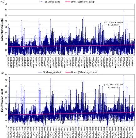
The trend of the night-time background ozone can be found, using night-time hourly ozone monitoring data collected from the period of 1998–2005 at various monitoring stations in the Sydney basin. To analyse all hourly ozone data, the linear regression method was used with ozone as an affine function of nitrogen oxide and the BOL is derived when the NO concentration is zero. Figure 2 shows an example of the results for St. Marys site, a suburban site in the west of Sydney. It reveals an increasing trend with an increasing rate in the ozone concentration of 3.2±0.3 ppb (standard error is 0.3 ppb) over the 1998–2005 period (or 0.43±0.04 ppb per year) with a zero probability (p-value) obtained for the null hypothesis of the slope and an intercept of 15.6±0.2 ppb in the linear regression trend line, as shown in Figure 2(a).
(a)
(b)
Considering the level of oxidant, which consists of ozone (O3) and nitrogen dioxide (NO2), a similar upward trend can be observed as shown in Figure 2(b) with an increase of 4.6±0.3 ppb over the same period and intercept of 20.1±0.2 ppb in the linear regression trend line. Again the p-value is 0 for zero slope, and the oxidant concentration exhibits an increase on an average of 0.66±0.04 ppb per year.
The same trend is found in our analysis for all other sites in the Sydney basin, except at Lidcombe where the Lidcombe monitoring site was discontinued in mid 2002 and was replaced by a nearby station, a few streets away at Chullora. With a possible extension of data points up to 2005 using data collected at Chullora, a similar temporal profile could be obtained at Lidcombe in comparison to other stations.
As summer is the time when photochemistry is most active, only ozone data during that time of the year rather than of the whole year are used to determine BOL (Fiore et al., 2002). Indeed, our results show that there is not much difference in the trend lines from using only summer data and using all yearly data.
The Sydney background ozone trend is similar to the trend in United States and Europe. Indeed, Jaffe and Ray (2007) has reported similarly of the ozone trend at 11 remote rural sites in north and western United States (including Alaska), in which 7 sites show a statistically significant increase in ozone with an annual increase of 0.26 ppb on average. These sites are considered as ‘pristine’ background ozone sites. Temperature changes can account for only part of the trend, and the authors explained these trends coming possibly from increasing regional emissions, change in the distribution of emissions, increasing biomass burning or increasing global background ozone, and especially due to rapid growth in emissions within Northeast Asia. In the same context, Simmonds et al. (2004) shows an increasing trend in background ozone observations at Mace Head on the west coast of Ireland from 1987 to 2003 with an average of 0.49±0.19 ppb per year. They concluded that there has been at least one major perturbation of the ozone trend during the 1998–1999 timeframe that was associated with global biomass burning coupled to an intense El Ni˜no event of 1997.
4. Relationship between oxidant and nitrogen oxides in background ozone modelling
In the attempt to determine the BOL in the day-time photochemical condition and its trend from ambi-ent measuremambi-ents at local site conditions, this section describes the relationship between oxidant (including ozone and nitrogen dioxide, O3+NO2) and nitrogen oxides (NOx =NO+NO2) at various sites in the Syd-ney basin. The results obtained from the measurements, observed locally or regionally, can be extrapolated to find the derived background ozone at the local sites. Moti-vated by Clapp and Jenkin (2001), we will focus on
establishing a linear relationship between the average val-ues of oxidant and NOx levels from daily data collected respectively in daytime and night-time. Also, this oxidant level at a given location is made up of NOx-independent and NOx-dependent contributions. The NOx-independent contribution is the intercept, which equals the daytime background oxidant level, while the slope of the regres-sion line represents the NOx-dependent contribution or the level of primary pollution from the local sources. The analysis has covered the 6 year period from 1998 to 2003, collected in the Sydney region during the photochemistry-active summer in the Southern Hemisphere.
This approach of using the regression line to find the BOL is also similar to the one that Altshuller and Lefohn (1996) but instead of using the relationship between ozone and peroxyacetyl nitrate (PAN) as well as ozone versus total reactive nitrogen species (NOy) or ozone
versus (NOy− NOx), we use the relationship between oxidant (ozone+nitrogen dioxide)versusNOxas outlined by Clapp and Jenkin (2001). The reason is that most ambient monitoring stations do not measure PAN or NOy and this situation is the case in the Sydney basin.
4.1. Local background oxidant level analysis
Using data for the summer 1998 period at monitoring sites in the Sydney basin, the plots of daylight average (O3+NO2) versus NOx are shown in Figure 3, respec-tively for Blacktown, Bringelly, St. Marys, and Rich-mond. Most of these sites are considered as urban except for Richmond, which is located in a semi-rural area. A linear regression line can be fitted to the correspond-ing data as shown but some variance can be expected. This is explained by a major variation in the regional contributions resulting from frequent elevated levels of ozone during the summer period. Two separate regres-sion lines can be fitted to the ‘ozone non-episode’ and ‘ozone episode’ days (Clapp and Jenkin, 2001). Here, the episode day is defined as a day when one or more sta-tions in the Sydney basin has an ozone level greater than 80 ppb. The daytime background level for ‘non-episode’ and ‘episode’ days can be obtained from the intercepts of the regression lines.
Figure 3. Daytime oxidant levelversus NOxin Sydney West in 1998: broken (solid) lines for episode (non-episode) days.
Table II. Comparison between episode and non-episode background oxidant levels at Sydney basin sites in 1999.
Region Site Non-episode Episode
Background level (ppb)
Slope Background
level (ppb)
Slope
West Blacktown 15 0.65 16 1.95
Bringelly 16 0.95 14 2.25
St. Marys 21 0.40 37 0.70
Richmond 18 0.75 11 3.70
Bargo 13 0.45 32 0.60
Vineyard 17 1.15 17 3.10
Eastern Randwick 16 0.40 21 0.65
Rozelle 10 0.40 13 0.85
Earlwood 13 0.35 17 0.80
Woolooware 16 0.50 17 1.15
Central Lidcombe 16 0.40 23 1.25
Westmead 13 0.40 13 1.40
Liverpool 16 0.50 28 0.70
Lindfield 18 0.30 18 2.10
Average 15.5 0.54 19.8 1.51
non-episode days and about 55 ppb for episode ones. These values can be compared with the BOL value of about 35 ppb as reported by Oltmanset al. (2008) of air entering the west coast of the North America at Trinidad. Contrary to the findings using ambient data measured at Sydney West sites, the overall analysis for east Sydney sites, such as Randwick and Rozelle, does not show a distinct relation between oxidant (O3 and NO2) and nitrogen oxides (NOx) and the scatter around the regression lines appears to be relatively large. Under the photo-stationary assumption for photochemical reactions,
it is generally expected a linear relationship between oxidant and nitrogen oxide levels. This means the ideal photo-stationary state of smog reaction rarely occurs in the east Sydney area.
Table III. Comparison between episode and non-episode background oxidant levels at Sydney basin sites in 2000.
Region Site Non-episode Episode
Background level (ppb) Slope Background level (ppb) Slope
West Blacktown 18 0.65 17 1.85
Bringelly 16 1.45 15 2.25
St. Marys 22 0.40 37 0.75
Richmond 21 0.85 10 3.80
Bargo 21 0.85 32 0.65
Vineyard 22 0.45 18 3.10
Eastern Randwick 20 0.50 21 0.60
Rozelle 18 0.40 13 0.85
Earlwood 18 0.50 17 0.85
Woolooware 15 1.15 17 1.10
Central Lidcombe 19 0.45 22 1.30
Westmead 16 0.60 13 1.40
Liverpool 21 0.35 28 0.65
Lindfield 19 0.40 18 2.10
Average 19.0 0.64 19.9 1.52
the rate of change in background oxidant level with respect to the NOx concentration (slope). In average, the derived background oxidant for the Sydney area is about 16 ppb for non-episode days and about 4 ppb higher for the episode days. Generally, the daytime BOL was more consistent during the non-episode days because it has a small change between 10 and 20 ppb while for episode days, the level varies from 11 to 37 ppb. However, only few sites like St. Marys, Bargo, Randwick, and Liverpool display a clear relationship for the local contribution of the oxidant level (NOx -dependent) in this year, as the slopes for regression lines between non-episode and episode days are about simi-lar. This implies that the local oxidant level depended on the local activities and pollution emissions, thus its trends varied from site to site and also between episode and non-episode days. It is also noted that the NOx -dependent contribution apparently existed at the semi-rural inland sites such as Vineyard, Richmond, and Bringelly (with higher value of slopes). The reason was probably due to the long-range transportation of the ozone produced due to emission from the industrial activities and vehicle transports in the coastal area to these inland sites.
Table III shows the derived results for background oxidant level in the year 2000. On average, the non-episode level was 3 ppb higher than the previous year. However, there were not much changes in the level for the episode days. Furthermore, the local contributions also followed similar trends as in year 1999 but with slightly higher values. A clear oxidant-NOx relationship between episode and non-episode days can be observed at St. Marys and Bargo (in the west Sydney), Randwick, Earlwood and Woolooware (in the east Sydney), and Liverpool (in the central of Sydney). Nevertheless, the results for these 3 years 1998–2000 show that the ideal photo-stationary state cannot be achieved at every site due
to some variations of the local contributions, especially during the episode days.
In the subsequent 5 year analysis from 2001 to 2005, we focus on the NOx-independent contributions. From Table IV, the upward tendency of the daytime back-ground oxidant level did occur generally for the non-episode days, except for Westmead and Linfield (in the central part of Sydney). For the episode days, there were some sites that show an upward trend such as Bringelly, Bargo, and Vineyard, all located at the west of Sydney, and are consistent with the findings stated above. How-ever, the background oxidant level at some other sites was observed to vary irregularly for each year.
4.2. Background oxidant level trend
Table IV. Episode and non-episode background oxidant levels at Sydney basin sites from 2001 to 2005.
Region Site Non-episode background level (ppb) Episode background level (ppb)
2001 2002 2003 2004 2005 2001 2002 2003 2004 2005
West Blacktown 22 23 24 ∗ ∗ 30 20 24 ∗ ∗
Bringelly 21 21 19 32 37 15 32 32 50 56
St. Marys 22 24 23 39 38 22 19 33 53 57
Richmond 21 26 25 38 38 35 24 26 45 55
Bargo 20 23 21 27 31 19 29 32 44 45
Vineyard 27 25 29 38 38 17 18 28 43 42
Eastern Randwick 21 21 22 20 24 25 28 23 22 22
Rozelle 21 20 20 20 20 25 20 17 38 27
Earlwood 20 19 20 20 24 21 21 21 53 50
Woolooware 20 19 21 ∗ ∗ 21 20 27 ∗ ∗
Central Lidcombe ∗ ∗ ∗ 30 (Chullora) 33 (Chullora) ∗ ∗ ∗ 49 (Chullora) 52 (Chullora)
Westmead 24 18 22 ∗ ∗ 29 13 23 ∗ ∗
Liverpool 24 ∗ 17 20 35 27 – 15 58 58
Lindfield 25 18 22 30 ∗ 33 25 37 60 ∗
Average 22.2 21.4 21.9 28.5 31.8 24.5 22.4 26.0 46.8 46.4
Asterisk represents the non-available data for the correspondence year.
Figure 4. Daytime background oxidant trend for non-episode days at several Sydney sites from 1998 to 2005. The overall comparison for the defined BOL for
1998–2005 data (e.g. for St. Marys site) using several methods is now summarized in Table V. It is clear that methods 2 and 3 show similar level of the night-time and daytime background oxidant, however, higher values occurred in 2004 and 2005 using the C–J method. This partially confirms the validity of our proposed approach for the determination of BOL. Furthermore, the annual BOL increase (in ppb/year) by using the C–J linear trend line is slightly higher, whereas a consistent trend is observed by the proposed methods 1 and 2. As shown, an offset of about 5 ppb exists consistently between the night-time background ozone and the night-time oxidant (O3+NO2) to account for the nitrogen dioxide concentration.
Figure 5. Daytime background oxidant trend for episode days at several Sydney sites from 1998 to 2005.
Table V. Background ozone level determination (in ppb) at St. Marys using several methods.
Methods 1998 1999 2000 2001 2002 2003 2004 2005 Trend
(ppb/year)
1 Night-time background ozone (daily average night-time when NO=0)
15.6 16.0 16.5 16.9 17.3 17.8 18.2 18.6 +0.43
2 Night-time background oxidant (daily average night-time when NO=0)
20.1 20.8 21.4 22.1 22.7 23.4 24.1 24.7 +0.66
3 Daytime background oxidant for non-episode days (by C–J method)
20.0 21.0 22.0 22.0 24.0 23.0 39.0 38.0 +2.63
4 Daytime background oxidant for episode days (by C–J method)
27.0 37.0 37.0 22.0 19.0 33.0 53.0 57.0 +3.27
to tropospheric ozone. Notably, the upward trend reported in this article for the local BOL in Sydney is also in line with the results obtained by Jaffe and Ray (2007) in the United States and by Simmonds et al. (2004) in Europe.
Currently, the ozone standards for one-hourly average and four-hourly average ozone concentrations in Aus-tralia are 100 and 80 ppb, respectively. In the Sydney basin, there are several exceedances above the one-hourly standard each year. Efforts have been made to reduce the number of exceedances through emission control of motor vehicles, domestic and commercial sources of oxides of nitrogen (NOx) and Volatile Organic Com-pounds (VOCs) notwithstanding the increase of popu-lation and the number of motor vehicles in the basin. Most ozone level exceedances have occurred in the west, northwest, and southwest with a relatively higher BOL in Sydney northwest compared to other parts of Sydney.
5. Discussion and conclusion
This article has presented some refinements of the BOL definition and presented measurement-based methods to determine the time and daytime BOL. The night-time BOL as the average of ambient measurements of
hourly ozone values from night-time to early morning when NO is not present for at least 2 h consecutively. Ambient air quality data collected at monitoring sites in the Sydney basin are used to derive the local BOL and to investigate the BOL trend over the years. The night-time BOL results have been compared with a method to estimate the background oxidant concentration introduced by Clapp and Jenkin (2001).
From the analysis, there is a clear upward trend in background ozone concentration at nearly all Sydney monitoring sites. For other regions, such as the Lower Hunter in the north and Illawarra in the south of the Sydney basin, the BOL and their trends can be determined and the results may be different from that of Sydney as the BOL (and hence its trend) is depending on a number of conditions such as the meteorological flow, pollution sources, and terrain conditions in those regions. Altshuller and Lefohn (1996) derived BOL at many different coastal and inland sites in the United States and Canada. They found that the concentration of background ozone varies as a function of geographic area, elevation, season, and averaging time. They also suggested that the different ranges of derived BOL is accounted for by the BOL’s dependence on a number of conditions such as the nature of upwind flow, lack of pollution sources, and terrain conditions including deposition with respect to forest or agricultural areas at those sites.
From the local or regional scale, considerations can be made to the background ozone on a continental scale and hence the result of background ozone trend in this article may be compared and related to the trend in the background ozone observation measured at Cape Grim, in Tasmania (Australia). Cape Grim is located at the southern end of the Australian continent and is mostly unaffected by anthropogenic sources. There is a strong coupling of surface ozone at Cape Grim and the tropo-sphere ozone during the winter months. An increasing trend of background ozone at Cape Grim from 1982 to 2003 is detected from about 24 to 26 ppb (Galballyet al., 2005). As suggested by Oltmans et al. (2006), changes in air mixed down from the troposphere above to the surface could play a role in the change of ozone seen at Cape Grim in the mid latitude Southern Hemisphere. This upward trend in background ozone at Cape Grim is also in line with results reported in the United States by Jaffe and Ray (2007) and in Europe by Simmondset al. (2004). The implication of this background ozone trend is believed to be important for the regulatory authorities in many countries in setting the ozone goal and target for emission reduction, as it may not be possible to act independently in the local and regional context without a coordinated action on the global scale to reduce also the emission of precursors. For example, if the current 1 h ozone standard is lowered, it would mean that the efforts and policy measures for reduction of the annual number of exceedance in the Sydney region can be less effective and it would be more difficult to keep the ozone level within the allowable threshold.
References
Altshuller AP, Lefohn AS. 1996. Background ozone in the planetary boundary layer over the United States. Journal of Air and Waste Management Association46(2): 134–141.
Chan E, Vet RJ. 2010. Baseline levels and trends of ground level ozone in Canada and the United States.Atmospheric Chemistry and Physics 10: 8629–8647.
Clapp L, Jenkin M. 2001. Analysis of the relationship between ambient levels of O3, NO2 and NO as a function of NOx in the UK. Atmospheric Environment35: 6391–6405.
Derwent RG, Stevenson DS, Doherty RM, Collins WJ, Sanderson MG. 2008. How is surface ozone in Europe linked to Asian and North American NOx emission. Atmospheric Environment 42: 7412–7422.
Diaz-de-Quijano M, Penuelas J, Ribas A. 2009. Increasing interannual and altitudinal ozone mixing ratios in the Catalan Pyrenees.
Atmospheric Environment43: 6049–6057.
Duc H, Azzi M. 2009. Analysis of background ozone in the Sydney basin. InProceedings of the 18th World IMACS/MODSIM 2009 Inter-national Congress on Modelling and Simulation. Cairns, Australia, 2307–2313, http://www.mssanz.org.au/modsim09/F10/duc.pdf. Fiore AM, Jacob DJ, Bey I, Yantosca RM, Field BD, Fusco AC.
2002. Background ozone over the United States in summer: Origin, trend, and contribution to pollution episodes.Journal of Geophysical Research107: 11.1–11.25.
Gadner MW, Dorling SR. 2000. Statistical surface ozone models: an improved methodology to account for non-linear behaviour.
Atmospheric Environment34: 21–34.
Galbally I, Meyer C, Bentley S. 2005. Trends in near-surface ozone at Cape Grim and in the Southern Hemisphere troposphere [electronic publication]. In: Towards a new agenda: 17th International Clean Air & Environment Conference proceedings, Hobart, Clean Air Society of Australia and New Zealand.
Hart M, de Dear R, Hyde R. 2006. A symnoptic climatology of tropospheric ozone episodes in Sydney, Australia. International Journal of Climatology26: 1635–1649.
Jaffe D, Ray J. 2007. Increase in surface ozone at rural sites in the western US.Atmospheric Environment41: 5452–5463.
Monks PS. 2003. TROTREP-Tropospheric ozone and precursors, trends, budgets and policy, synthesis and integration report.Report to the EU FPV Energy, Environment and Sustainable Development Pro-gram, European Union. http://www.le.ac.uk/chemistry/atmospheric/ pub.html.
Oltmans S, Lefohn A, Harris J, Galbally I, Scheel HE, Bodeker G, Brunke E, Claude H, Tarasick D, Johnson BJ, Simmonds P, Shadwick D, Anlauf K, Hayden K, Schmidlin F, Fujimoto T, Akagi K, Meyer C, Nichol S, Davies J, Redondas A, Cuevas E. 2006. Long-term changes in troposphere ozone.Atmospheric Environment 40: 3156–3173.
Oltmans SJ, Lefohn A, Harris J, Shadwick D. 2008. Background ozone levels of air entering the west coast of the US and assessment of long-term changes.Atmospheric Environment42: 6020–6038. Parrish DD, Millet DB, Goldstein AH. 2009. Increasing ozone in
marine boundary layer inflow at the west coasts of North America and Europe.Atmospheric Chemistry and Physics9: 1303–1323. Simmonds P, Derwent R, Manning A, Spain G. 2004. Significant
growth in surface ozone at Mace Head, Ireland, 1987–2003.
Atmospheric Environment38: 4769–4778.
U.S. Environmental Protection Agency. 2006. Air Quality Criteria for Ozone and Related Photochemical Oxidants (Final). Office of Research and Development: Research Triangle Park, EPA/600/R-05/004af. http://cfpub.epa.gov/ncea/cfm/recordisplay.cfm?deid= 149923.
U.S. Environmental Protection Agency. 2007.Review of the National Ambient Air Quality Standards for Ozone: Policy Assessment of Sci-entific and Technical Information OAQPS Staff Paper.Office of Air Quality and Planning and Standards: Research Triangle Park, EPA-452/R-07-003. www.epa.gov/ttn/naaqs/standards/ozone/data/2007 01 ozone staff paper.pdf.
Vingarzan R. 2004. A review of surface ozone background levels and trends.Atmospheric Environment38: 3431–3442.