WALKER, CHRISTOPHER CODY. Development of Accurate Coarse-grained Polymer Molecular Models and a Framework for Copolymer Sequence Characterization via the Kerr Effect. (Under the direction of Dr. Erik E. Santiso and Dr. Jan Genzer).
Copolymers, macromolecules which contain more than one type of monomer chemical unit, are highly versatile materials in that control over the spatial arrangement of comonomers along the chains can lead to a wide range of thermophysical properties. To explore this vast design space and understand structure-property relationships, molecular simulation and theoretical models are invaluable tools. A fundamental challenge in polymer modeling is capturing in a reasonable timeframe the wide breadth of time and length scales relevant to polymer dynamics. Systematic coarse-graining approaches, in which several atoms are grouped into effective interaction sites, aim to efficiently reproduce a subset of key properties from high-resolution simulations and/or experimental datasets.
In chapter 2, a new approach for developing accurate coarse-grained polymer force fields for molecular dynamics (MD) simulations is presented, which combines a powerful and
predictive group-contribution molecular equation of state (SAFT-γ Mie) with structural
solubility parameters and heat capacities with comparable or superior accuracy to all-atom models.
In chapters 3 and 4, the fused-sphere SAFT-γ Mie approach is applied to a complex copolymer system, poly(vinyl butyral-co-vinyl alcohol) (PVB), which is widely used in
laminated safety glass interlayers, due to a balance of adhesion of the vinyl alcohol monomers to hydroxylated silica surfaces and toughness imparted by the vinyl butyral monomers. A key goal of this work is to gain insight into the structure of the PVB-glass interface, and to investigate the role of comonomer sequence on PVB adhesion phenomena. To overcome a lack of experimental data, a group contribution approach was used to represent the VB monomer as a construct of chemical fragments from molecules with similar chemistries. Interactions with a realistic all-atom hydroxylated amorphous silica slab were mapped to an external potential acting on the coarse-grained beads, and MD simulations were systematically run for a series of vinyl alcohol contents and block length distributions of VA and VB monomers. Results indicate that adhesion strength of random-blocky PVB copolymers is determined not only by the number of VA segments contacting the surface, but is also strongly influenced by the morphology above the contacting layer. Surface chemical heterogeneity was also found to play a critical role. In copolymers with moderate VA content, highly blocky, but not diblock, copolymers, provided maximal adhesion energy.
Copolymer Sequence Characterization via the Kerr Effect
by
Christopher Cody Walker
A dissertation submitted to the Graduate Faculty of North Carolina State University
in partial fulfillment of the requirements for the degree of
Doctor of Philosophy
Chemical Engineering
Raleigh, North Carolina 2019
APPROVED BY:
_______________________________ _______________________________ Dr. Erik E Santiso Dr. Jan Genzer
Committee Co-chair Committee Co-chair
ii DEDICATION
iii BIOGRAPHY
Christopher Cody Walker was born on August 9th, 1992 in Mineola, New York to parents Robert and Vivian Walker. He grew up on Long Island in North Massapequa, NY along with his older sister Lindsay. Christopher attended Plainedge High School, where apart from academics he was heavily involved in several orchestral groups as a violinist, attaining the role of concert master in the 2009-10 season. After graduating from Plainedge in the spring of 2010, he began the pursuit of a bachelor’s degree in chemical engineering at the University of Notre Dame in South Bend, Indiana, following in the footsteps of Lindsay, who had two years prior joined the incoming class of 2008 to pursue a degree in computer science.
At Notre Dame, Christopher joined the Notre Dame Symphony Orchestra, and, naturally, developed a keen interest in Notre Dame football. It was not until late in his junior year at Notre Dame that he decided to pursue undergraduate research, when he joined the polymer chemistry lab of Dr. Ruilan Guo. There, he worked on the synthesis of novel polyimide copolymers for use in efficient gas separation membranes. In the summer of 2013, he took a hiatus from the Guo group to work as an undergraduate researcher in the group of Dr. Hsueh-Chia Chang, also at Notre Dame, on the development of a microfluidic biosensing platform for detection of viral RNA strands to be deployed in the developing world. In was these two research experiences that compelled Christopher to continue his academic career into graduate school.
In May of 2014, Christopher graduated cum laude with a bachelor’s degree in chemical engineering. The following fall, he joined the incoming class at North Carolina State University in Raleigh, NC to pursue a PhD in chemical engineering. There he joined the research groups of Dr. Erik Santiso and Dr. Jan Genzer to study computational and theoretical modeling of
iv ACKNOWLEDGMENTS
Firstly, I would like to acknowledge my advisors Dr. Erik Santiso and Dr. Jan Genzer, for their tremendous support, feedback, and encouragement these past five years. I am honored to be the first co-advised student in your two groups. Dr. Santiso, I am continually impressed by your knowledge of molecular simulations and statistical mechanics, and have learned a great deal. I am very grateful for the opportunities you’ve given me to travel to international conferences, which were highlights of my graduate school experience. Dr. Genzer, you’ve been a truly exceptional mentor, and your humor always brightens my workday. The G.I.R.L.S. (Genzer Interfacial Research Laboratory Students) beach retreats you’ve created and planned I will remember forever. I’d also like to especially thank Dr. Orlin Velev and Dr. Melissa Pasquinelli for serving as committee members and providing very useful feedback along the way.
In the Santiso research group: special acknowledgement I give to Dr. Amulya Pervaje, for our countless discussions on our day-to-day simulation problems and SAFT, and meeting for months on end writing and re-writing our review paper. This last year would have been so much harder without you. Dr. Nathan Duff, for our many useful discussions, your simulation advice, and your help with all things Henry2; Dr. Mariah King, for helping me learn Python and the basics in my early days in the group; Kaihang Shi, for all the great times travelling together in Scotland and Spain for the Thermodynamics conferences; Jennifer Clark, for all our atrium discussions and fun times outside of work; Dr. Laura Weiser; Dr. Deepti Srivastava; Dr. Chengxiang Liu; Dr. Amit Mishra; Dr. Cody Addington; Matt Mansell; Rakshit Jain; and Van Nguyen.
v atrium together – the successes you’ve achieved are so inspiring. To all those past and present who have given me valuable feedback in many a group meeting, and especially those who attended our incredibly fun and very memorable beach retreats: Dr. C.K. Pandi, Dr. Kunal Mondal, Dr. Kirill Efimenko, Dr. Rohan Patil, Dr. Preeta Datta, Dr. Edwin Walker, Dr. Ying Liu, Dr. Duncan Davis, Dr. Yiliang Lin, Dr. Matt Melillo, Dr. Gilbert Castillo, Dr. Jason Miles, Dr. Russell Schmitz, Yeongun Ko, Steven Zboray, Shreya Erramilli, Camden Cutright, Srivatsan Ramesh, Sunyoung Woo, Eduardo Barbieri, and Bradley Davis.
Dr. Alan Tonelli, for our insightful discussions about the Kerr effect calculations and rotational isomeric state theory; Dr. Shanshan Li, for teaching me about the Kerr effect
experiments; and Srivatsan for running Kerr effect experiments to help validate my theoretical calculations.
Dr. Gregory Parsons, for acting as a third research advisor and mentor during my time working in the Parsons research group on density functional theory calculations of atomic layer etching reactions; Dr. Wenyi Xie, for our discussions about ALD and ALE chemistry.
Dr. David Ollis, Dr. Jason Haugh, Dr. Keith Gubbins, Dr. Peter Fedkiw, for excellent teaching of the core graduate courses, and all of the CBE staff, especially Sandra Bailey and Michelle Bunce.
To the Eastman Chemical Company for funding the project that led to much of the results presented in this dissertation, and all those who have provided guidance and feedback in our project meetings and helped in the approval process for my presentations and publications.
vi Others at NC State outside of my research groups who I’d like to acknowledge: Amanda Volk, Leah Granger, Dr. Charles (Chas) McGill, Dr. Chris Straub, Dr. Joseph Tilly, Ria Corder, C.J. Duran, Barbara Farias, Dr. Ashton Lavoie, Ryan Maloney, Dr. Jonathan Conway, and Dr. Yiming Wang.
To all of my conference friends, for our very useful discussions about SAFT-γ Mie and amazing adventures in Scotland and Spain.
To all of my CHEG friends from Notre Dame, and all our insanely late nights studying which helped me to understand the foundations of chemical engineering and get me to where I am today.
vii TABLE OF CONTENTS
LIST OF TABLES ... xi
LIST OF FIGURES ... xiv
Chapter 1: Introduction and background ... 1
1.1. Motivation ... 1
1.2. Copolymer sequence dictates material properties ... 3
1.3. Methods for characterizing copolymer sequences ... 4
1.4. Overview of molecular dynamics and force fields ... 8
1.5. Coarse-graining strategies or polymers ... 13
1.5.1. Bottom-up coarse-graining ... 15
1.5.2. Top-down and hybrid coarse-graining ... 19
1.6. The SAFT-γ Mie Equation of State ... 22
1.7. Chapter Overviews ... 25
1.8. References ... 28
Chapter 2: Development of a fused-sphere SAFT-γ Mie force field for poly(vinyl alcohol) and poly(ethylene) ... 43
2.1. Abstract ... 43
2.2. Introduction ... 44
2.3. The SAFT-γ Mie Equation of State ... 46
2.4. Fused-sphere SAFT-γ Mie EoS ... 48
2.5. Extending SAFT-γ Mie to rigid polymers ... 49
2.6. SAFT-γ Mie EoS parameterization ... 50
2.7. SAFT-γ Mie parameter validation by direct MD simulation of the vapor-liquid interface ... 53
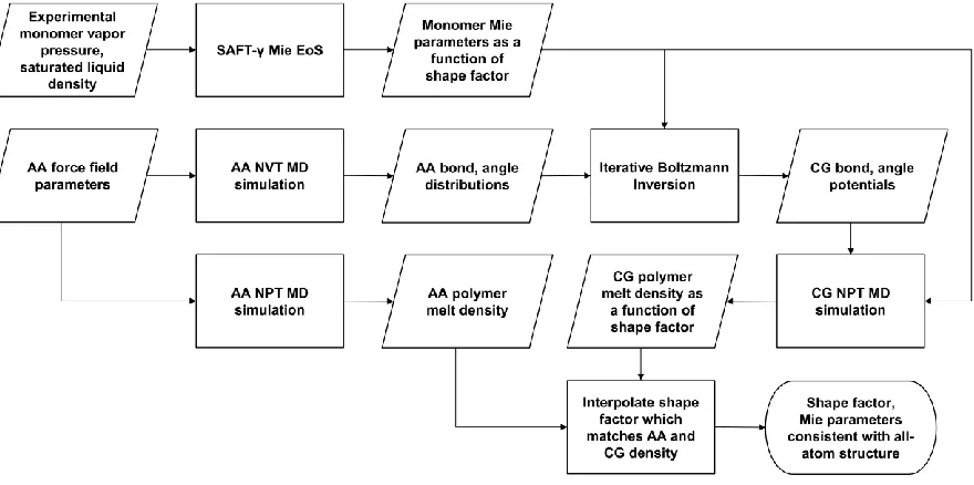
2.8. Deriving effective bonded potentials from all-atom simulations ... 54
2.9. SAFT-γ Mie shape factor from polymer density matching ... 59
2.10. Force field validation ... 66
2.10.1. Hildebrand solubility parameter ... 66
2.10.2. Heat Capacity ... 69
2.10.3. Radius of gyration and end-to-end distance distributions ... 70
2.10.4. Persistence length ... 73
2.10.5. Glass transition temperature ... 74
2.11. Conclusions and Future Work ... 77
2.12. References ... 79
Chapter 3: Extending the fused-sphere SAFT-γ Mie force field parameterization approach to poly(vinyl butyral) copolymers ... 86
3.1. Abstract ... 86
3.2. Introduction ... 87
viii 3.4. Validation of SAFT-γ Mie parameters by MD simulation of the vapor-liquid
interface ... 99
3.5. Adding bonded potentials from all-atom MD simulation ... 101
3.6. PVB force field validation and discussion ... 110
3.6.1. Glass transition temperature ... 110
3.6.2. Heat capacity... 114
3.7. Reverse-mapping ... 115
3.8. Conclusions ... 118
3.9. References ... 121
Chapter 4: The effect of poly(vinyl butyral) co-monomer sequence on adhesion to amorphous silica: a coarse-grained molecular dynamics study ... 129
4.1. Abstract ... 129
4.2. Introduction ... 130
4.3. Simulation methods ... 136
4.3.1. Fused-sphere SAFT-γ Mie force field ... 136
4.3.2. Force-mapping silica-PVB interactions ... 138
4.3.3. Coarse-grained PVB adsorption MD simulation ... 141
4.4. Results and discussion ... 143
4.5. Conclusions ... 154
4.6. Acknowledgements ... 157
4.7. References ... 158
Chapter 5: A framework for copolymer sequence characterization via calculation of the theoretical molar Kerr constant ... 165
5.1. Introduction and motivation ... 165
5.2. Measuring the Kerr constant of polymer solutions ... 166
5.3. Theoretical background ... 169
5.3.1. Bond polarizability additivity (valence optical scheme) ... 170
5.3.2. Polymer rotational isomeric state theory ... 171
5.3.3. Matrix multiplication scheme ... 174
5.3.4. Calculation of mK for vinyl polymers ... 178
5.4. A brief history of modern polymer Kerr effect literature ... 180
5.5. Methods and Matlab code validation... 186
5.5.1. Overview of Matlab code ... 186
5.5.2. Validation of literature <r2> values ... 187
5.5.2.1. Polyethylene ... 187
5.5.2.2. Poly(ethylene terephthalate) (PET) ... 188
5.5.2.3. Generic 3-state vinyl substituted polymers ... 189
5.5.2.4. Poly(vinyl chloride) ... 191
5.5.3. Validation of literature <μ2> values ... 192
5.5.3.1. Poly(vinyl chloride) ... 192
5.5.3.2. Poly(styrene-co-p-bromostyrene) ... 194
ix
5.5.4.1. Poly(styrene-co-p-bromostyrene) ... 196
5.5.4.2. Poly(vinyl chloride) ... 199
5.6. Conclusions and future directions ... 200
5.7. References ... 204
Chapter 6: Conclusions and outlook ... 209
6.1. Modeling polymers with fused-sphere SAFT-γ Mie coarse-grained models ... 209
6.2. Interfacial behavior of PVB copolymers with complex sequences ... 211
6.3. Future work for the Kerr effect ... 212
6.4. References ... 213
Appendices ... 214
Appendix A: Supporting information for chapter 2 ... 215
A.1. Force field parameters for OPLS-AA and COMPASS simulations ... 215
A.1.1. Poly(ethylene) OPLS parameters ... 217
A.1.2. Poly(vinyl alcohol) OPLS parameters ... 218
A.1.3. Poly(ethylene) COMPASS parameters ... 220
A.1.4. Poly(vinyl alcohol) COMPASS parameters ... 224
A.2. Temperature dependence of effective bond and angle distributions ... 230
A.3. Testing bonded potentials for optimal fused-sphere SAFT-γ Mie models... 232
A.4. Converged effective bond and angle potentials from iterative Boltzmann inversion ... 234
A.5. Detailed fused-sphere SAFT-γ Mie parameterization results ... 236
A.6. Mie parameter empirical correlations with shape factor ... 237
A.7. Density profiles from vapor-liquid equilibria MD simulation ... 238
A.8. References ... 239
Appendix B: Fused-sphere SAFT-γ Mie Equation of State governing equations ... 240
B.1. Overview ... 240
B.2. Ideal gas contribution ... 241
B.3. Monomer contribution ... 241
B.3.1. Hard sphere monomer term ... 242
B.3.2. First perturbation monomer term ... 243
B.3.3. Second perturbation monomer term... 245
B.3.4. Third perturbation monomer term ... 247
B.4. Chain contribution ... 247
B.5. References ... 251
Appendix C: Supporting information for chapter 3 ... 253
C.1. Force field parameters for OPLS-AA simulations ... 253
C.2. Converged effective bond and angle potentials from iterative Boltzmann inversion ... 257
C.3. Detailed fused-sphere SAFT-γ Mie parameterization results ... 260
x
C.5. Extended PVB copolymer density results ... 264
C.6. PVB solubility parameter calculation ... 267
C.7. References ... 269
Appendix D: Supporting information for chapter 4 ... 270
D.1. Contact maps of PVB coarse-grained beads with the silica surface ... 270
xi LIST OF TABLES
Table 1.1. Summary of data used to develop various top-down and hybrid CG force fields. .. 21
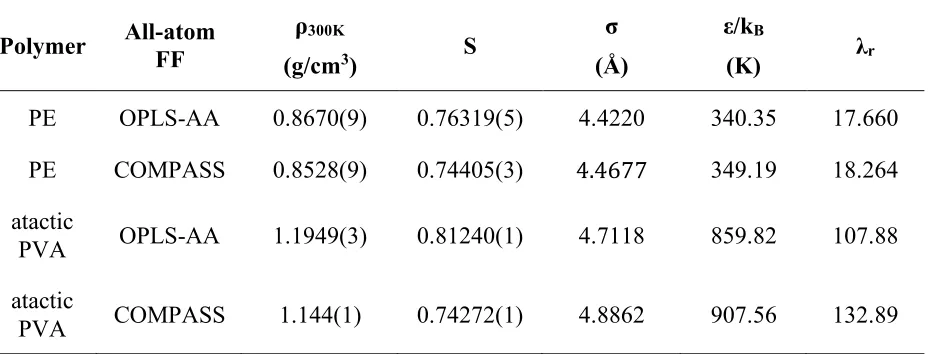
Table 2.1. Tangent SAFT-γ Mie parameters for PE and PVA monomers... 52
Table 2.2. Fused-sphere SAFT-γ Mie parameters for PE and PVA 24-mers. ... 64
Table 2.3. Hildebrand solubility parameters for SAFT-γ Mie PVA and PE models at T=300 K. OPLS and COMPASS refer to the all-atom force field used to fit the bonded parameters. ... 67
Table 2.4. Constant pressure heat capacity per monomer for SAFT-γ Mie PVA and PE models at 300 K. OPLS and COMPASS refer to the all-atom force field used to fit the bonded parameters... 69
Table 2.5. Persistence lengths of SAFT-γ Mie and all-atom atactic PVA models at 500 K and 700 K. ... 74
Table 2.6. Hyperbolic fitting parameters for PVA volume vs. temperature MD data. ... 76
Table 3.1. Tangent SAFT-γ Mie parameters for PVB fragments... 97
Table 3.2. Fused-sphere SAFT-γ Mie parameters for PVB fragments. ... 110
Table 3.3. Hyperbolic fitting parameters for PVB density vs. temperature MD data. ... 112
Table 4.1. Chemical compositions of the PVB chains. ... 142
Table 5.1. Comparison between calculated characteristic ratios of polyethylene chains with varying amounts of backbone bonds. ... 188
Table 5.2. Comparison between calculated theoretical molar Kerr constant ratios for various sequences of multiblock PS-co-PBrS copolymers. ... 198
Table A.1.1.1. Atom types and non-bonded parameters for OPLS PE. ... 217
Table A.1.1.2. Bond parameters for OPLS PE. ... 217
Table A.1.1.3. Angle parameters for OPLS PE. ... 217
Table A.1.1.4. Torsion parameters for OPLS PE. ... 217
Table A.1.2.1. Atom types and non-bonded parameters for OPLS PVA. ... 218
xii
Table A.1.2.3. Angle parameters for OPLS PVA. ... 218
Table A.1.2.4. Torsion parameters for OPLS PVA. ... 219
Table A.1.3.1. Atom types and non-bonded parameters for COMPASS PE. ... 220
Table A.1.3.2. Atom type equivalences for COMPASS PE. ... 220
Table A.1.3.3. Bond increment parameters for COMPASS PE. ... 220
Table A.1.3.4. Quartic bond parameters for COMPASS PE. ... 221
Table A.1.3.5. Quartic angle parameters for COMPASS PE. ... 221
Table A.1.3.6. Bond-bond parameters for COMPASS PE. ... 221
Table A.1.3.7. Bond-angle parameters for COMPASS PE. ... 221
Table A.1.3.8. Torsion parameters for COMPASS PE. ... 222
Table A.1.3.9. Middle-bond-torsion parameters for COMPASS PE. ... 222
Table A.1.3.10. End-bond-torsion parameters for COMPASS PE. ... 222
Table A.1.3.11. Angle-torsion parameters for COMPASS PE... 223
Table A.1.3.12. Angle-angle-torsion parameters for COMPASS PE. ... 223
Table A.1.3.13. Angle-angle parameters for COMPASS PE. ... 223
Table A.1.4.1. Atom types and non-bonded parameters for COMPASS PVA. ... 224
Table A.1.4.2. Atom type equivalences for COMPASS PVA. ... 224
Table A.1.4.3. Bond increment parameters for COMPASS PVA. ... 225
Table A.1.4.4. Quartic bond parameters for COMPASS PVA. ... 225
Table A.1.4.5. Quartic angle parameters for COMPASS PVA. ... 225
Table A.1.4.6. Bond-bond parameters for COMPASS PVA. ... 226
Table A.1.4.7. Bond-angle parameters for COMPASS PVA. ... 226
xiii
Table A.1.4.9. Middle-bond-torsion parameters for COMPASS PVA... 227
Table A.1.4.10. End-bond-torsion parameters for COMPASS PVA... 227
Table A.1.4.11. Angle-torsion parameters for COMPASS PVA. ... 228
Table A.1.4.12. Angle-angle-torsion parameters for COMPASS PVA. ... 228
Table A.1.4.13. Angle-angle parameters for COMPASS PVA. ... 229
Table A.5.1. Fused-sphere SAFT-γ Mie parameterization results for 2-site n-butane. ... 236
Table A.5.2. Fused-sphere SAFT-γ Mie parameterization results for 2-site 1,3-butanediol. ... 236
Table A.6.1. Fitting coefficients for normalized sigma parameter correlation. ... 236
Table A.6.2. Fitting coefficients for normalized epsilon parameter correlation. ... 236
Table A.6.3. Fitting coefficients for normalized repulsive exponent correlation. ... 236
Table C.1.1. Atom types and nonbonded parameters for OPLS PVB. ... 254
Table C.1.2. Bond parameters for OPLS PVB. ... 255
Table C.1.3. Angle parameters for OPLS PVB. ... 255
Table C.1.4. Torsion parameters for OPLS PVB. ... 256
Table C.3.1. Fused-sphere SAFT-γ Mie parameterization results for 2-site n-butane. ... 260
Table C.3.2. Fused-sphere SAFT-γ Mie parameterization results for 2-site 1,3-butanediol. ... 260
Table C.3.3. Fused-sphere SAFT-γ Mie parameterization results for 2-site 2,5-dimethyltetrahydrofuran. ... 261
Table C.3.4. Fused-sphere SAFT-γ Mie parameterization results for 3-site paraldehyde. ... 261
Table C.3.5. Fused-sphere SAFT-γ Mie parameterization results for 4-site 1,4-dioxane... 262
Table C.4.1. Fitting coefficients for normalized sigma parameter correlation... 262
Table C.4.2. Fitting coefficients for normalized epsilon parameter correlation. ... 263
xiv LIST OF FIGURES
Figure 1.1. Illustration depicting variables in the polymer materials design space, examples of different copolymer sequence arrangements, and physical properties which are highly dependent on polymer chemical structure. ... 3 Figure 1.2. Depiction of simulation methods used for different time and length scales. The
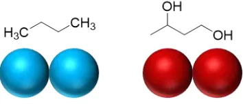
top-down coarse-graining approach based on the SAFT-γ Mie equation of state, and Boltzmann inversion, a bottom-up approach, are used in this dissertation to bridge the time and length scales shown. Modified from reference 88. ... 15 Figure 2.1. Mapping scheme for PE and PVA dimers from n-butane and 1,3-butanediol,
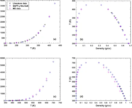
respectively. ... 52 Figure 2.2. Vapor pressure curve (a) and vapor-liquid phase envelope (b) for the tangent
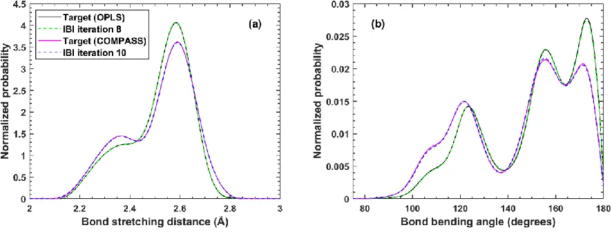
dimer SAFT-γ Mie n-butane system with 135,000 molecules. Vapor pressure curve (c) and vapor-liquid phase envelope (d) for the 1,3-butanediol system with 145,000 molecules. Error bars are smaller than the symbol size and are not shown. ... 54 Figure 2.3. Bond stretching (a) and angle bending (b) distributions for PE 250-mers
converged to all-atom targets using IBI at T=400 K. Solid black lines are the target distributions mapped from the OPLS force field and solid magenta lines are the target distributions mapped from the COMPASS force field. Dashed green lines are the converged CG bonded distributions for the OPLS targets after 8 iterations of IBI. Dashed blue lines are the converged CG distributions for the COMPASS targets after 10 iterations of IBI. The converged tabulated
potentials are provided in the supplemental material. ... 57 Figure 2.4. Bond stretching (a) and angle bending (b) distributions for atactic PVA
250-mers converged to all-atom targets using IBI at T=400 K. Solid black lines are the target distributions mapped from the OPLS force field and solid magenta lines are the target distributions mapped from the COMPASS force field. Each target distribution is the average over three all-atom chains with independent stereochemistry distributions. Dashed green lines are the converged CG bonded distributions for the OPLS targets after 14 iterations of IBI. Dashed blue lines are the converged CG distributions for the COMPASS targets after 10 iterations of IBI. ... 58 Figure 2.5. Optimized Mie parameters for fixed shape factors, normalized by the parameter
values for the tangent model (S=1.0). Optimal σ Mie parameters (a) are fit to a power law in S, ε Mie parameters (b) are fit to a second-order polynomial in S, and repulsive exponent (λr) Mie parameters (c) are fit to a third-order
xv coefficients for each of the empirical fits are reported in the supplementary
information... 60 Figure 2.6. Algorithm for fused-sphere SAFT-γ Mie polymer force field parameterization. .... 61 Figure 2.7. Simulated polymer density of PE (a) and PVA (b) 24-mers at T=300 K and 1
atm with the Mie potential defined by the optimal parameters for each shape factor. All density values are the average of 3 independent simulations with different starting configurations. Error bars are smaller than the symbol size and not shown. For PVA, the S=0.6 parameter set was not used in the density matching due to numerical issues with the extremely high repulsive exponent. The all-atom systems for PE and PVA contain 100 and 90 chains, respectively, while the coarse-grained systems are 4 times larger. ... 62 Figure 2.8. Chain length (N) dependence of optimal shape factor for the atactic PVA model
with bonded potentials and all-atom density from the OPLS force field. The total number of monomers in the system was kept constant over all chain
lengths (8,640 for coarse-grained simulations, 2,160 for all-atom simulations). .... 65 Figure 2.9. End-to-end distance (a) and radius of gyration (b) distributions for SAFT-γ Mie
and OPLS all-atom PE 24-mer melts at 500 K. The lines are fits to a spline
interpolant. ... 71 Figure 2.10. End-to-end distance (a) and radius of gyration (b) distributions for SAFT-γ Mie
and COMPASS all-atom PE 24-mer melts at 500 K. ... 71 Figure 2.11. End-to-end distance (a) and radius of gyration (b) distributions for SAFT-γ Mie
and OPLS all-atom PVA 24-mer melts at 700 K. ... 72 Figure 2.12. End-to-end distance (a) and radius of gyration (b) distributions for SAFT-γ Mie
and COMPASS all-atom PVA 24-mer melts at 700 K. ... 72 Figure 2.13. Volume versus temperature data from the cooling NPT MD simulations for the
SAFT-γ Mie PVA models based on structural detail from (a) OPLS and (b)
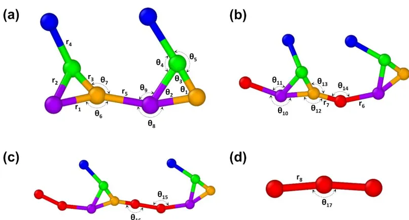
COMPASS, fit to a hyperbolic switching function (Equation (2.10)). ... 76 Figure 3.1. Group contribution scheme for constructing the PVB copolymer (f) from
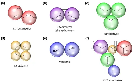
compounds with sufficient data available. For paraldehyde (c) and 1,4-dioxane (d), halves of oxygen atoms are mapped to each bead. ... 94 Figure 3.2. PVB Mie parameter correlations based on a series of optimizations for fixed
values of shape factor. (a) Optimized σ Mie parameters, normalized by the tangent values σ(S=1.0), fit to a power law in S. (b) Normalized ε Mie parameters fit to a second-order polynomial in S. (c) Normalized λ Mie
xvi Figure 3.3. Vapor pressure curve (a) and vapor-liquid phase envelope (b) for DMTHF 2-site
tangent-sphere SAFT-γ Mie model (108,000 molecules). ... 100 Figure 3.4. Vapor pressure curve (a) and vapor-liquid phase envelope (b) for paraldehyde
3-site tangent-sphere SAFT-γ Mie model with ring correction to the chain term
(97,000 molecules). ... 101 Figure 3.5. Vapor pressure curve (a) and vapor-liquid phase envelope (b) for 1,dioxane
4-site tangent-sphere SAFT-γ Mie model with ring correction to the chain term (18,900 molecules). Deviation from the EoS values are likely due to the
weakening of the torsion potential relative to thermal energy. ... 101 Figure 3.6. Effective bond and angle definitions shown for all possible copolymer
sequences: (a) SAFT-γ Mie PVB dimer (b) 2 repeat units of PVB alternating AB copolymer (c) 2 repeat units of PVB alternating AAB copolymer (d) PVA trimer. ... 103 Figure 3.7. Converged effective bond stretching distributions for the coarse-grained
SAFT-γ Mie PVB chains after IBI at T=400 K. Each coarse-grained chain has a length corresponding to 500 carbons. Targets mapped from OPLS-AA polymer chains are shown as solid black lines, and distributions resulting from the converged
CG potentials are shown as dashed magenta lines. ... 105 Figure 3.8. Converged effective angle-bending distributions for the coarse-grained SAFT-γ
Mie PVB chains after IBI at T=400 K. Side chain angles θ4 and θ5 are omitted, having been replaced by Mie nonbonded interactions to improve overall convergence. Targets mapped from OPLS-AA polymer chains are shown as solid black lines, and distributions resulting from the converged CG potentials are shown as dashed magenta lines. ... 106 Figure 3.9. Absolute error against all-atom density (in g/cm3) for PVB SAFT-γ Mie
homopolymer (a) and PVB SAFT-γ Mie random 50:50 copolymer (b) as a function of the ring-type shape factor (S1) and side chain shape factor (S2), estimated from short MD simulations, fit to a 2d 2nd order polynomial. The sum of errors for (a) and (b) are given in (c), indicating that there is no solution for (S1,S2) which satisfies both PVB homopolymer and 50:50 copolymer target densities. The sum of all copolymer density errors (25, 50, 75 mol % PVA random copolymers, and 50 mol % diblock copolymer) are given in (d), indicating excellent transferability of shape factors to various copolymer
compositions. ... 108 Figure 3.10. Density dependence on shape factor for PVB 50:50 random copolymer with
S1=S2, obtained from the average of 3 well-equilibrated (30-60 ns) NPT simulations comprising 120 PVB chains. The optimal shape factor for PVB is determined by interpolation of a quadratic fit to match the all-atom density,
xvii Figure 3.11. Glass transition sequential cooling MD simulation results for random PVB
copolymers containing various amounts of vinyl alcohol content. Solid lines are the 5-parameter hyperbolic fits given by Equation (3.8). ... 112 Figure 3.12. Comparison of simulated glass transition temperatures of PVB copolymers
with literature values.59,60,84 Error bars are the 95 % confidence interval from the hyperbolic fitting. ... 113 Figure 3.13. Constant pressure heat capacity of PVB copolymers and PVA homopolymer37
at 300 K, per mol of monomers, calculated from SAFT-γ Mie MD simulation (black circles), compared with literature data (blue diamonds).86,87 Uncertainties for the MD data points assigned based on block-averaging are smaller than the symbol size. ... 115 Figure 3.14. Comparisons between radii of gyration at 300 K of fused-sphere SAFT-γ Mie
PVB copolymer chains and reverse-mapped OPLS-AA systems after energy minimization. Red open circles represent each of the 240 PVB chains for a given copolymer composition, and dashed black lines represent equal Rg in the CG and AA systems. Root-mean-square deviation (RMSD) is shown to
represent deviation from perfect Rg matching. ... 117 Figure 3.15. Illustration of superimposed SAFT-γ Mie and reverse-mapped OPLS-AA PVB
copolymer chains with 50 mol% vinyl alcohol content. The chain configurations are taken from a bulk 240-chain system at 300 K, and the all-atom chain is shown after the energy minimization step. CG bonds are shown in black, AA bonds and atoms are shown in cyan, and CG beads represented by their Mie
radii scaled by S1/3 are colored as in Fig. 3.6. ... 118 Figure 4.1. Expected influence of PVB blockiness on adhesion strength and interfacial
toughness. ... 132 Figure 4.2. Monomer chemical structures of PVB, and examples of comonomer sequences
resulting from different blockiness parameters, with 50 mol% of each monomer type. ... 135 Figure 4.3. Coarse-grained SAFT-γ Mie model for PVB copolymers. The parent molecules
of each bead and mapping function are given in chapter 3 (ref. 60). The coarse-grained beads are bonded at all points of co-tangency shown, and angle
potentials are used for all possible angles except those involving the side chain alkyl bead shown in dark blue, which retains instead nonbonded interactions
with 1-3 neighbors. For clarity, bead overlap is not depicted here. ... 137 Figure 4.4. Top-down (top) and cross-sectional (bottom) view of all-atom amorphous silica
xviii Figure 4.5. Mean VA (a) and VB (b) block lengths for 25 mol% VA (blue), 50 mol% VA
(black), and 75 mol% VA (red) copolymer chains of fixed molecular weight
~2.4kDa. Error bars are the standard deviation of the 3 independent trials. ... 142 Figure 4.6 Visualization of 3D morphology for PVB copolymers at the interface with silica
(located at the lower region at approximately z = 20 Å), as function of VA content and blockiness parameter used to generate the comonomer sequences. One of the three independent trials is shown as a representative example of each VA content and blockiness. Red beads represent VA monomers, and semi-transparent cyan beads represent VB monomers. All beads are depicted as spheres with diameters equal to their equilibrium Mie self-interaction distance, scaled by their shape factors, and all simulation snapshots are taken after 150 ns of equilibration at 400 K. ... 145 Figure 4.7. Contact fraction of VA monomers on the force-mapped silica surface as a
function of x, y, VA content, and blockiness, histogrammed over a 100 ns sampling period at 400 K. The 2D colormaps correspond to the same selected trials as the 3D morphologies in Fig 4.6. We considered a monomer as
contacting if it contains a bead whose lowest point lies within a 1 Å cutoff
distance from a surface map. ... 146 Figure 4.8. Adhesion energy, in (a) kcal per mol of beads and (b) J/m2, for the PVB-silica
interface as a function of blockiness for varying amounts of VA, and the numbers of (c) VA and (d) VB monomers contributing to the PVB-silica interaction energy. The numbers of contributing beads were defined by an energy cutoff of 1E-3 cal/mol. The value of adhesion energy for PVA
homopolymer (417.9 ± 0.6 J/m2) is omitted from the J/m2 plot for clarity of the copolymer data. Likewise, omitted from plot (c) is the number of interacting VA monomers for the PVA homopolymer (1089 ± 1). In all cases averages are computed over the last 10 ns of the 150 ns simulation period at 400 K, and error bars represent the standard deviation amongst the 3 independent trials. ... 149 Figure 4.9. (a) Scalar contact fractions corresponding to the 2D contact area plots in Fig.
4.7, averaged over all 3 independent trials. (b) Fractional contribution from the VA beads to overall adhesion energy, using an energy per mol of beads basis. ... 150 Figure 4.10. Average number of chains containing at least 1 adsorbed monomer as a
function of blockiness for given VA monomer contents. Averages are taken
over the last 100 ns at 400 K, and over the 3 independent trials. ... 151 Figure 4.11. Average numbers of VA monomers in (a) trains, (c) loops, (e) tails and VB
monomers in (b) trains, (d) loops, (f) tails per adsorbed chain (i.e., normalized by the data in Fig. 4.10) as a function of blockiness for given VA monomer contents. Averages are taken over the last 100 ns at 400 K, and over the 3
xix Figure 4.12. Average overall volume fraction of VA monomers within all (a) trains, (b)
loops, and (c) tails as a function of blockiness for given VA monomer contents. Averages are taken over the last 100 ns at 400 K, and over the 3 independent
trials. Monomer volumes are defined by their Mie radii as described earlier. ... 154 Figure 5.1. Schematic for polymer solution Kerr effect experimental setup. Image is taken
from reference 3. ... 167 Figure 5.2. Depiction of a segment of a vinyl polymer chain exhibiting different side chain
stereochemistries. Adapted from reference 23. ... 179 Figure 5.3. Flowchart illustrating the information required by the RIS/matrix multiplication
Matlab program, and algorithm for calculation of the theoretical molar Kerr
constant. ... 186 Figure 5.4. Repeat unit of PET, shown with parameters for the RIS model of Williams and
Flory,48 reproduced from the entry in reference 22. The physical significance
and values of the γ and σ RIS parameters are described therein. ... 189 Figure 5.5. Comparison of our calculated characteristic ratio for PET (left) with the original
results of Williams and Flory (right).48 ... 189 Figure 5.6. Comparison of our calculated characteristic ratios (right) for various vinyl
polymer models studied by Flory, Mark, and Abe9,49 with their original results (left). In each case, the vinyl polymers contain 100 repeat units. In our
calculations, averages were taken over 10,000 chains with independent
stereosequences. ... 190 Figure 5.7. Comparison of our calculated characteristic ratios (right) for various vinyl
polymer models with the original results of Tonelli (left).9 In each case, chains contain 400 repeat units. In our calculations, averages were taken over 500 chains with independent stereosequences. The averages in the figure by Tonelli are taken over either 10 or 20 chains. ... 191 Figure 5.8. Comparison of our calculated characteristic ratios (right) for PVC against the
results of Mark (left).50 In each case the PVC chains are 100 repeat units in length. We used 500 chains with independent stereosequences to generate the averages. The plot by Mark also depicts the results for a polypropylene model. The nomenclature used for isotactic replication probability by Mark (pr) is
synonymous with the ωiso parameter. ... 192 Figure 5.9. Comparison of our calculated dipole moment ratios (right) for PVC as a
xx Figure 5.10. Comparison of our calculated dipole moment ratios for PVC (right) as a
function of racemic replication probability against the results of Khanarian et al12 (left). Chain lengths are 200 repeat units, and we averaged over 500 chains. Note that in the plot by Khanarian, dipole moment ratio is shown on the right y axis, while the Kerr constant of PVC (which we compare in section 5.5.4.2) is on the left y axis. Models A and B are represented by solid and dashed lines, respectively. In this case, the notation Pr is used to represent racemic replication probability (i.e., the probability of adding a monomer with opposite chirality to the previous). The units for the dipole moment ratio axes are equivalent in the two plots. The RIS parameter η varied in the two different models is a first-order parameter representing the propensity of the backbone carbon atoms for the trans conformation,50 and Δφ is as described above. ... 194 Figure 5.11. Comparison of our calculated dipole moment ratios (right) for
poly(styrene-co-p-bromostyrene) as a function of the fraction of brominated monomers, with the results of Khanarian et al. (left). In each case, chains with 200 repeat units were generated such that they contained 55% racemic dyads. In the plot by
Khanarian, dipole moments are in units of Debyes, black squares represent experiment dipole moment measurements for PS-co-PBrS, and white squares represent experimental results for the chlorinated analog, poly(styrene-co-p-chlorostyrene). Our values were taken as the average over 5,000 independently generated chains. ... 195 Figure 5.12. Calculated molar Kerr constants of poly(styrene-co-p-bromostyrene)
copolymers of varying brominated monomer fraction and fraction of racemic dyads (pr), with degree of polymerization of 200 repeat units. Left: results from our Matlab code, with each point taken as the average of 5,000 independently generated chains. Right: the original results reported by Khanarian et al.33 Units of mK on the y axes are equivalent. Our calculations are in quantitative
agreement with those of Khanarian, using the same polystyrene RIS model,52 bond dipole moments, and bond polarizability tensors. Black squares in the plot of Khanarian correspond to experimental Kerr constant measurements. ... 197 Figure 5.13. Calculated molar Kerr constants of PS homopolymers of varying racemic dyad
fractions as a function of molecular weight. For each molecular weight,
averages are taken over 5,000 chains with independent stereosequences. ... 199 Figure 5.14. Comparison of our calculated theoretical mK for PVC (right) as a function of
racemic replication probability against the results of Khanarian et al12 (left). Chain lengths are 200 repeat units, and we averaged over 500 chains. Models A and B are represented by solid and dashed lines in the left plot, respectively. The units for the mK axes are equivalent in the two plots. The RIS parameters η and Δφ are as in Fig 5.10... 200 Figure A.2.1. Temperature dependence of the (a) effective bond stretching and (b) effective
xxi a PE OPLS 250-mer in vacuum. Distributions are averaged over a 40 ns
production period following 10 ns equilibration, fit to a spline interpolant. ... 230
Figure A.2.2. Temperature dependence of the (a) effective bond stretching and (b) effective bond bending angle distributions for PE SAFT-γ Mie monomers mapped from a PE COMPASS 250-mer in vacuum. Distributions are averaged over a 40 ns
production period following 10 ns equilibration, fit to a spline interpolant. ... 230
Figure A.2.3. Temperature dependence of the (a) effective bond stretching and (b) effective bond bending angle distributions for PVA SAFT-γ Mie monomers mapped from the average of 3 atactic PVA OPLS 250-mers in vacuum with independent distributions in stereochemistry. Distributions are averaged over a 30 ns
production period following 20 ns equilibration, fit to a spline interpolant. ... 231 Figure A.2.4. Temperature dependence of the (a) effective bond stretching and (b) effective
bond bending angle distributions for PVA SAFT-γ Mie monomers mapped from the average of 3 atactic PVA COMPASS 250mers in vacuum with independent distributions in stereochemistry. Distributions are averaged over a 30 ns
production period following 20 ns equilibration, fit to a spline interpolant. ... 231
Figure A.3.1. Ability of the optimized PE SAFT-γ Mie + OPLS model to capture
temperature dependence of (a) effective bond stretching and (b) effective bond bending angle distributions of isolated 250-mers is vacuum. Note that the Boltzmann inversion was performed only at T=400 K using the tangent SAFT-γ Mie parameters. Distributions are averaged over a 40 ns production period following 10 ns equilibration, fit to a spline interpolant. Remarkably, the non-bonded potential allows the model to accurately capture the sharpening of the peak at ~175 degrees at 300 K. ... 232
Figure A.3.2. Ability of the optimized PE SAFT-γ Mie + COMPASS model to capture temperature dependence of (a) effective bond stretching and (b) effective bond bending angle distributions of isolated 250-mers is vacuum. Note that the Boltzmann inversion was performed only at T=400 K using the tangent SAFT-γ Mie parameters. Distributions are averaged over a 40 ns production period
following 10 ns equilibration, fit to a spline interpolant. ... 232
Figure A.3.3. Ability of the optimized PVA SAFT-γ Mie + OPLS model to capture
xxii Figure A.3.4. Ability of the optimized PVA SAFT-γ Mie + COMPASS model to capture
temperature dependence of (a) effective bond stretching and (b) effective bond bending angle distributions of isolated 250-mers is vacuum. Note that the Boltzmann inversion was performed only at T=400 K using the tangent SAFT-γ Mie parameters. Distributions are averaged over a 30 ns production period following 20 ns equilibration, fit to a spline interpolant. Each distribution is the average from 3 250mers with independent distributions in stereochemistry. ... 233
Figure A.4.1. Converged (a) effective bond stretching and (b) effective bond bending angle potentials for the SAFT-γ Mie PE model at T=400 K with target distributions mapped from the OPLS all-atom 250-mer MD simulations. The potentials are bounded by harmonic wells to deal with ranges of values not sampled in the MD simulations. ... 234 Figure A.4.2. Converged (a) effective bond stretching and (b) effective bond bending angle
potentials for the SAFT-γ Mie PE model at T=400 K with target distributions mapped from the COMPASS all-atom 250-mer MD simulations. ... 234 Figure A.4.3. Converged (a) effective bond stretching and (b) effective bond bending angle
potentials for the SAFT-γ Mie PVA model at T=400 K with target distributions mapped from the OPLS all-atom 250-mer MD simulations. ... 235 Figure A.4.4. Converged (a) effective bond stretching and (b) effective bond bending angle
potentials for the SAFT-γ Mie PVA model at T=400 K with target distributions mapped from the COMPASS all-atom 250-mer MD simulations. ... 235 Figure A.7.1. Density profiles for tangent SAFT-γ Mie dimers extracted from vapor-liquid
equilibria MD simulations for (a) 135,000 n-butane molecules and (b) 145,000 1,3-butanediol molecules. For each temperature, spatial averages are taken over the last 2 ns of a 20 ns NVT simulation of the vapor-liquid interface. Density profiles are fit to a 4-parameter hyperbolic tangent function as described in reference 8. The density profiles for the two vapor-liquid interfaces are fit separately, and the final values of saturated vapor and liquid density are taken as the average of both fits. Shown here are the averaged profiles reflected about
z=0. ... 238 Figure C.2.1. Converged effective bond stretching potentials for the SAFT-γ Mie PVB
copolymer model at T=400 K with target distributions mapped from the OPLS all-atom MD simulations. Bond types are defined in Figure 3.6. The potentials are bounded by harmonics to deal with ranges of values not sampled in the MD simulations. These harmonics are parameterized to be C2 continuous with the splines. ... 257 Figure C.2.2. Converged effective angle bending potentials for the SAFT-γ Mie PVB
xxiii are bounded by harmonics to deal with ranges of values not sampled in the MD simulations. These harmonics are parameterized to be C2 continuous with the splines. ... 258 Figure C.2.3. Angle bending distributions at T=400 K for CG angle types 4 and 5 (cf. Figure
3.6) resulting from Mie 1-3 nonbond interactions, with all other PVB
homopolymer bonded potentials converged. We were unable to converge these angles using iterative Boltzmann inversion, due to the the removal of the
stereochemical features which give rise to the peaks in the distributions mapped from OPLS-AA simulations. For θ4, the potential from direct inversion of the all-atom distribution leads to poor sampling in the high-angle region. The application of steep potentials to shift θ4 towards larger angles resulted in numerically unstable simulations. For θ5, direct inversion fails to capture the largest peak, while much improvement is made by instead using the Mie 1-3
interactions. ... 259 Figure C.5.1. Colormaps depicting absolute error (in g/cm3) between SAFT-γ Mie
coarse-grained density and OPLS-AA density from NPT simulations, as a function of the ring bead shape factors (S1) and the alkyl side chain bead shape factor (S2). For both OPLS-AA and SAFT-γ Mie, densities are the average over 3
simulations with independent stereochemistry and starting configurations. SAFT-γ Mie densities are sampled from the final 200 ps in the polymatic
compression-annealing algorithm.7 ... 264 Figure C.5.2. The effect of the two vinyl butyral shape factor parameters (S1,S2) on the Mie
potential for intermolecular interactions involving the side chain bead: (a) Mie potential for interactions between n-butane and DMTHF bead types with S1 = S2; (b) Mie potential for interactions between n-butane and DMTHF bead types with S1 ≥ S2; (c) Mie potential for interactions between n-butane and DMTHF bead types with S1 ≤ S2; (d) Mie potential for interactions between n-butane and paraldehyde bead types with S1 = S2; (e) Mie potential for interactions between n-butane and 1,4 dioxane bead types with S1 = S2. ... 266 Figure C.6.1. Comparison of solubility parameters calculated from MD (black diamonds),
literature data for commercial PVB resins (red squares), and group contribution estimates11 with various vinyl alcohol contents. MD simulations were performed at 300 K, and the Hansen group contribution correlations for the commercial
resins were developed at 298 K. ... 268 Figure D.1. Contact maps of each of the 5 PVB coarse-grained bead types with the
xxiv the coarse-grained contact maps, these were obtained from MD simulations of
adsorbed PVB or PVA homopolymer melts at 400 K. The base of the silica slab model is located near z = 0. The coarse-grained bead contact maps are smoothed using the user-created Matlab smoothn function available through the Matlab
File Exchange. ... 270 Figure D.2. One-dimensional volume fraction profiles of VA monomers as a function of z
coordinate (i.e., distance from the silica surface) and blockiness for (a) 25 mol% VA, (b) 50 mol% VA, and (c) 75 mol% VA. Averages are taken over 100 ns at 400 K, and the average of the 3 trials is shown. ... 271 Figure D.3. Contributions from the (a) VA and (b) VB monomers to the total adhesion
energy shown in Fig. 4.8... 272 Figure D.4. Loop length distributions for (a) 25 mol% VA, (c) 50 mol% VA, (e) 75 mol%
VA, and train length distributions for (b) 25 mol% VA, (d) 50 mol% VA, (f) 75 mol% VA as a function of blockiness (100 ns average at 400 K over 3 trials). The length distributions of tails, of which there are far fewer than trains and
loops, are not sufficiently sampled to be of use. ... 273 Figure D.5. Average numbers of (a) trains, (b) loops, and (c) tails per adsorbed chain as a
1 CHAPTER 1
Introduction and background
Parts of this chapter have been published in Molecular Simulation 2019, 45 (14-15), 1223-1241
1.1. Motivation
Polymers, macromolecules made up of one or more types of monomer chemical units, have revolutionized the materials industry. Since the boom of the synthetic polymer industry in the mid-twentieth century, they have become ubiquitous in our everyday lives. Today, rapid progress is being made at the forefront of polymer synthetic chemistry in creating increasingly elaborate architectures and precise sequence patterns in copolymers for specialized
applications.1–4 A world of opportunity exists for improving current copolymer materials, and creating new ones, by manipulating their chemical sequences and spatial arrangement of monomers. Newfound tools for materials design such as machine learning, combined with advances in molecular simulation, accelerate the pace at which optimal polymer sequences and structural motifs for a given application may be found, as well as offer guidance to
experimentalists on how such copolymers might be physically realized. Yet, few studies to date have ventured beyond the realm of random, alternating, and diblock copolymers to determine structure-property relationships in synthetic copolymers with irregular sequences.
2 necessitates the use of scale approaches to fully capture their behavior. This topic of multi-scale polymer modeling has received a great deal of attention in recent years, and much progress has been made in bridging the gaps between quantum chemistry calculations, atomistic force fields, coarse-grained models, and macroscale models.5–8 However, further work in this area is still needed. In a 2017 National Science Foundation (NSF) report9 on frontiers in polymer science, the following grand challenge was posed:
“To develop new tools – experimental and computational methods and theory – and leverage them in an integrated way across any relevant length scales and time scales to accurately measure, predict, and elucidate underlying connections among structure, properties, and dynamics of any macromolecular system.”
Additionally, the importance of achieving sequence characterization with monomer-level precision was stressed:9
“Advances in polymer synthesis have outpaced advances in characterizing monomer sequence at the single-chain level. An associated challenge, therefore, is the accurate determination of monomer sequence and topology in polymers. Indeed, the challenges go hand-in-hand – accurate determination of sequence will be a critically important
analytical tool for efforts to control sequence precisely.”
3 potential method for identifying polymer microstructure by measurement of electric
birefringence (Kerr effect) of polymer solutions, and interpretation of the results by a theoretical framework which relates polymer conformation, dipole moments, and polarizability at the atomic level, to macroscopic properties.
1.2. Copolymer sequence dictates material properties
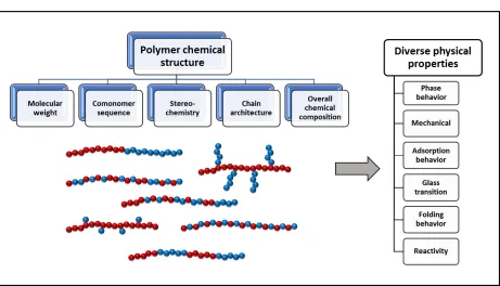
Figure 1.1. Illustration depicting variables in the polymer materials design space, examples of different copolymer sequence arrangements, and physical properties which are highly dependent on polymer chemical structure.
4 structure-property relationships in model systems such as diblock or random copolymers are now generally well understood, further studies are needed to achieve the same level of knowledge for new types of copolymers with complex sequences.
1.3. Methods for characterizing copolymer sequences
5 of comonomer placement is controlled through manipulation of reaction conditions, and
sequence-defined copolymers, which have perfect sequences.40,41
A combination of many tools will likely be needed to achieve complete sequencing of higher-molecular-weight synthetic copolymers. At the most basic level of characterization, the overall relative amounts of two or more types of monomer could be distinguished by elemental analysis if each contains a distinctive element – for example, if one monomer type is
halogenated, and another type is not. In 13C NMR, identification of stereosequences up to pentad level, but comonomer sequences at only dyad or triad levels, is typical.31 This is possible in large part due to the γ-gauche effect, in which magnetic shielding differs depending on the rotational state of substituent groups.42 More nuanced NMR methods such as kinetic modeling during controlled radical polymerization,43 or clever design of the polymer chemistry such that signal may be enhanced by the presence of π-π stacking, for example,44 can provide additional insight for comonomer sequencing. Designing complementary strands which selectively bind to specific supramolecular motifs has even allowed for ‘frameshift reading’ of sequences,45 in mimicry of natural cellular machinery.
Mass spectrometry (MS) methods, including electrospray ionization (ESI),
6 fragmented and analyzed in a second MS stage. Fragmentation patterns of oligomers of specific sequences can in principle be used to fingerprint them.47 Impressive progress has recently been reported in this area to read the sequences of non-natural sequence-defined oligomers.33,38 However, further advances in the interpretation of the immensely complex MS/MS datasets are needed to parse long-range sequences.47 Advances in this emerging field of ‘polymeromics’, polymer science’s response to genomics and proteomics, are outlined in a recent review by Altuntaş and Schuberty.48 Tracking the degradation kinetics and products in certain copolymer systems may be another avenue to identifying sequences. For example, poly(lactic-co-glycolic acid) copolymers with different controlled comonomer sequences were found to exhibit dramatically different degradation behavior.29,30
The Kerr effect, or electric birefringence of polymer solutions, is potentially an extremely useful tool for characterization of sequences. Electric birefringence is the difference in refractive indices of an anisotropic material parallel (𝑛∥) and perpendicular (𝑛⊥) to the direction of an applied electric field (𝐸):
𝛥𝑛 = 𝑛∥− 𝑛⊥ = 𝐵𝜆𝐸2 (1.1)
7 showed promise for identifying the constituent components, a rather unique feat.54,55 The molar Kerr constant is related to macroscopic refractive index (𝑛), dielectric constant (𝜀), and density (𝜌), all at infinite dilution.
𝑚𝐾 = 6𝜆𝑀𝐵
(𝑛2+ 2)2(𝜀 + 2)2𝜌 (1.2)
To obtain this insight into polymer microstructure, the molar Kerr constant derived from the experiment must be interpreted by a theory that relates its conformational characteristics, local dipole moment, and local polarizability at the atomistic or monomer level, to observed birefringence. The theoretical molar Kerr constant is given by the following relation to overall polymer dipole moment (𝜇) and polarizability tensor (𝛼̂):
𝑚𝐾 = ( 2𝜋𝑁𝐴
135𝑘𝐵𝑇) [(
⟨𝜇𝑇𝛼̂𝜇⟩
𝑘𝐵𝑇 ) + ⟨𝛼̂
𝑅𝛼̂′𝐶⟩] (1.3)
The bracketed quantities represent conformational averages which can be calculated using rotational isomeric state (RIS) theory,56 which describes rotational potentials along the polymer backbone, and a matrix multiplication scheme developed chiefly by Nobel Laureate Paul Flory.57 Superscripts R and C denote row and column representations of the polarizability tensor, and 𝛼̂′ denotes the static polarizability tensor, distinguished from the optical
8 1.4. Overview of molecular dynamics and force fields
In molecular dynamics, the positions of interacting atoms or particles are tracked over finite time steps by numerical integration of Newton’s equations of motion. Though a variety of integrator schemes are commonly used in MD software packages, all are rooted in Taylor series approximations of position, velocity, and acceleration at time 𝑡 + 𝛥𝑡:58
𝑟(𝑡 + 𝛥𝑡) = 𝑟(𝑡) + 𝛥𝑡𝑣(𝑡) +1 2𝛥𝑡
2𝑎(𝑡) +1
6𝛥𝑡
3𝑏(𝑡) + 1
24𝛥𝑡
4𝑐(𝑡) … (1.4)
𝑣(𝑡 + 𝛥𝑡) = 𝑣(𝑡) + 𝛥𝑡𝑎(𝑡) +1 2𝛥𝑡
2𝑏(𝑡) +1
6𝛥𝑡
3𝑐(𝑡) … (1.5)
𝑎(𝑡 + 𝛥𝑡) = 𝑎(𝑡) + 𝛥𝑡𝑏(𝑡) +1 2𝛥𝑡
2𝑏(𝑡) + ⋯ (1.6)
In the above equation, 𝑏 and 𝑐 are the third and fourth derivatives of position with respect to time. One of the most widely used integration schemes is the velocity-Verlet method,59 which is favored for its high ratio of precision to computational cost, and the fact that it provides
positions, velocities, and accelerations at every time step, unlike many earlier algorithms.58 Interactions between particles are governed by a force field, usually taking a
predetermined analytical form. This can range anywhere from simple hard-sphere repulsion (excluded volume) interactions, as was used in the very first MD simulation by Alder and Wainwright in 1957,60 to complex polarizable models.61 As the goal of a force field is to faithfully represent the underlying physics of a molecular system, force field parameters are usually fit to potential energy surfaces from quantum mechanical calculations and/or
9
𝑈𝑡𝑜𝑡𝑎𝑙 = 𝑈𝑛𝑜𝑛𝑏𝑜𝑛𝑑+ 𝑈𝑏𝑜𝑛𝑑 + 𝑈𝑎𝑛𝑔𝑙𝑒+ 𝑈𝑡𝑜𝑟𝑠𝑖𝑜𝑛+ 𝑈𝑖𝑚𝑝𝑟𝑜𝑝𝑒𝑟 (1.7) Bond stretching potentials describe the potential energy of a bond as a function of bond distance, and thus prescribe the restoring force that should be applied when a bond deviates from its equilibrium distance. Bond angle-bending potentials are similar but describe the potential energy of angles defined by a central atom and two atoms bonded to it. Torsions, also referred to as ‘dihedrals,’ apply to groups of 4 atoms. For a group of atoms ijkl, defined by a central bond jk, a ‘proper’ torsion describes the potential energy of the angle defined by two planes ijk and jkl. Improper torsions instead govern the relative positions of 3 atoms bonded to a central atom, quantified by the angles amongst the 3 planes. Proper torsions may be used to impose backbone rigidity in chain molecules, for example, while improper torsions are useful for enforcing planarity and orientation of side groups, such as the phenyl groups in polystyrene chains.
Nonbonded potentials describe the interactions of all particles in the system, typically as a function of pairwise distances. A classic example, the Lennard-Jones 12-6 potential, includes a repulsive term which scales as 1/r12 and an attractive term which scales as 1/r6.
𝑈𝑖𝑗𝐿𝐽 = 4𝜀𝑖𝑗[(
𝜎𝑖𝑗
𝑟𝑖𝑗)
12
− (𝜎𝑖𝑗 𝑟𝑖𝑗)
6
] (1.8)
10 A more general form of the LJ 12-6 function with variable repulsive (𝜆𝑟) and attractive (𝜆𝑎) exponents, the Mie potential (Equation (1.9)), will be used extensively in this dissertation due to its improved versatility at describing interactions of real molecules.
𝑈𝑖𝑗𝑀𝑖𝑒 = 𝜀𝑖𝑗𝐶𝑖𝑗[(𝜎𝑖𝑗 𝑟𝑖𝑗)
𝜆𝑟
− (𝜎𝑖𝑗 𝑟𝑖𝑗)
𝜆𝑎
] 𝐶𝑖𝑗 = ( 𝜆𝑟 𝜆𝑟− 𝜆𝑎) (
𝜆𝑟 𝜆𝑎)
(𝜆𝜆𝑎
𝑟−𝜆𝑎)
(1.9)
Nonetheless, many atomistic force fields still use the LJ 12-6 potential due to its historical prevalence. Nonbonded interactions are typically not applied to particles directly bonded together or separated by 1 particle, as these are instead described by bonded potentials. Various force fields have adopted different conventions for scaling 1-4 nonbonded interactions.62–68 For charged systems, coulombic interactions are added, commonly of the following form:
𝑈𝑖𝑗𝑐𝑜𝑢𝑙 =𝑞𝑖𝑞𝑗
𝜖𝑟𝑖𝑗 (1.10)
In Equation (1.10), 𝑞𝑖 is the charge assigned to particle 𝑖 and 𝜖 is the dielectric constant of the medium. Most all-atom force fields assign partial charges to each atom, which may also depend on other atoms to which they are bonded, to better reproduce potential energy surfaces
determined from ab initio calculations. Coulombic interactions are much longer-range than the dispersion interactions described above, as evident by the 1/r scaling. An efficient means of capturing these long-range interactions is by solving the relevant equations in reciprocal space (‘k-space’) across infinitely many periodic images. Examples of this are Ewald summation58 and particle-particle-particle mesh (PPPM)69 solvers, both of which are widely implemented in molecular dynamics software packages.
11 field based in statistical associating fluid theory. OPLS is a ‘class I,’ or quadratic, all-atom force field, which uses a harmonic form for bond and angle potentials:
𝑈𝑏𝑜𝑛𝑑 = 𝐾𝑏(𝑟 − 𝑟𝑜)2 (1.11)
𝑈𝑎𝑛𝑔𝑙𝑒 = 𝐾𝜃(𝜃 − 𝜃𝑜)2 (1.12)
Proper torsions are described by a truncated Fourier series:
𝑈𝑡𝑜𝑟𝑠𝑖𝑜𝑛 =
𝐾𝜑,𝑖
2 [1 + 𝑐𝑜𝑠(𝜑 + 𝑓𝑖)] (1.13)
In OPLS, nonbonded interactions are the sum of both the LJ 12-6 function and coulombic term described above. COMPASS, a ‘class II’ all-atom force field, includes anharmonic analytical forms for bonded interactions and uses a softer 9-6 LJ function for nonbonded interactions. In addition to quartic bond and angle potentials (Equation (1.14)), cross-coupling terms for bond-bond, bond-angle, bond-torsion, angle-angle, angle-torsion, and angle-angle-torsion correlations are included. For example, the bond stretching potential and bond-angle coupling terms are given by the following:
𝑈𝑏𝑜𝑛𝑑 = 𝐾𝑏,2(𝑏 − 𝑏𝑜)2+ 𝐾𝑏,3(𝑏 − 𝑏𝑜)3 + 𝐾𝑏,4(𝑏 − 𝑏𝑜)4 (1.14)
𝑈𝑏𝑜𝑛𝑑−𝑎𝑛𝑔𝑙𝑒 = 𝐾𝑏𝜃(𝑏 − 𝑏𝑜)(𝜃 − 𝜃𝑜) + 𝐾𝑏′𝜃(𝑏′ − 𝑏𝑜′)(𝜃 − 𝜃𝑜) (1.15)
In Equation (1.15), 𝑏𝑜 and 𝑏𝑜′ are the equilibrium bond distances for the two bonds making up angle 𝜃 with equilibrium angle of 𝜃𝑜. A more complete description of the form of the
COMPASS force field is given in Appendix A and reference 63. Class II force fields were originally developed to model molecules with strained ring geometries,72–74 and in many cases the anharmonic terms are necessary to accurately predict vibrational spectra. They have also proved useful for modeling semiflexible polymers, whose complex intramolecular interactions are better described than with class I force fields.63,75–78 As one would expect, however,
12 tedious, and requires large datasets from ab initio calculations and experimental thermophysical properties. Availability of class II force field parameters for many polymer chemistries remains limited, especially bonded parameters which involve two dissimilar comonomer types.
In the SAFT-γ Mie coarse-grained force field,71 groups of atoms are represented by effective interaction sites. In the theory upon which SAFT-γ Mie is based, bonds are modeled as rigid and angle potentials are null, as in pearl necklace polymer models. A key goal of this work will be to incorporate realistic bond and angle potentials into SAFT-γ Mie polymer models, while preserving the link to thermodynamic data used to parameterize the SAFT-γ Mie equation of state.
In its natural form, MD simulations sample the microcanonical ensemble, in which number of particles (N), simulation cell volume (V), and total energy (E) are conserved. In most applications, however, a constant temperature (T), constant pressure (P), or both, are desired. To sample the NVT (isothermal) ensemble, a thermostat must be applied. Similarly, to sample the NPT (isothermal-isobaric ensemble), both a thermostat and barostat are needed. The Nosé-Hoover thermostat and barostat,79 which are widely accepted and implemented in most MD software packages, are used in this work. The Nosé-Hoover thermostat involves coupling the equations of motion to a heat bath, with artificial coordinates, velocities, and masses in an extended dimension allowing for sampling of the true canonical ensemble at a constant
temperature. In addition, the deterministic nature of a MD simulation is preserved, in contrast to approaches which involve stochastic collisions with a heat bath.79 In the NVT ensemble,
13 To reduce the effects of finite size of the simulation cell, which at best may span tens to hundreds of nanometers in atomistic simulations, periodic boundary conditions are commonly applied. Thus, a particle passing through one edge of the simulation cell reappears at the opposite end, and interactions spanning the boundaries must be properly accounted for following the minimum image convention. Nonetheless, systems sizes should be chosen to be large enough to reduce, or ideally eliminate, the effect of finite size. Parallelization of MD codes, typically by spatial decomposition to distribute the computational load across numerous processors, have enabled the study of massive molecular systems. Much progress has also been made in the area of graphics processing unit (GPU)-accelerated molecular dynamics software, even in the last 5 years since the start of the author’s research in this area. MD simulation of systems containing 10’s to 100’s of thousands of atoms or particles is now commonplace using standard high-performance computing platforms; with large-scale infrastructure, billion-atom simulations or millisecond time scales are achievable.
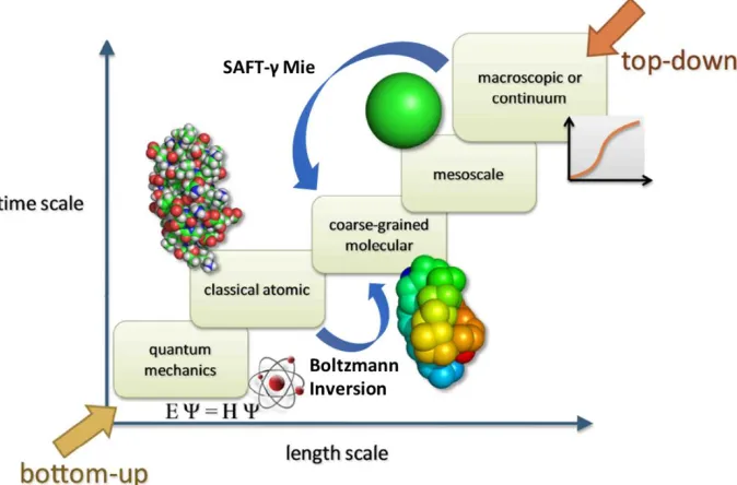
1.5 Coarse-graining strategies or polymers
Polymer dynamics span many orders of magnitude in both time and space, ranging from bond vibrations (femtoseconds, Angstroms) to macroscopic phenomena such as phase separation or self-assembly/folding (seconds, microns). With typical time steps for all-atom molecular dynamics simulations limited to approximately 1 fs by the frequencies of bond vibrations, it is not feasible even with modern supercomputing resources to capture these slower, larger-scale polymer phenomena in a reasonable timeframe. Coarse-graining approaches strive to improve computational efficiency by removing degrees of freedom compared to higher-resolution
14 thermophysical data. Dramatic speedups are achieved by grouping atoms into effective
15 Figure 1.2. Depiction of simulation methods used for different time and length scales. The top-down coarse-graining approach based on the SAFT-γ Mie equation of state, and Boltzmann inversion, a bottom-up approach, are used in this dissertation to bridge the time and length scales shown. Modified from reference 88.
1.5.1. Bottom-up coarse-graining
Bottom-up methods rely on data from high-resolution simulations to determine the coarse-grained potentials which best reproduce this data. All properties of the all-atom system cannot be preserved due to the reduction in the number of degrees of freedom, so target properties must be chosen carefully. The most widely used bottom-up coarse-graining
16
𝑈𝑖+1𝐶𝐺(𝑟) = 𝑈𝑖𝐶𝐺(𝑟) − 𝛼𝑘 𝐵𝑇𝑙𝑛 (
𝑔𝑖𝐶𝐺(𝑟)
𝑔𝐴𝐴(𝑟)) (1.16)
In which 𝑈𝑖𝐶𝐺(𝑟) is the interaction potential for the CG system at the ith iteration, kB is
Boltzmann’s constant, T is the temperature, 𝑔𝑖𝐶𝐺(𝑟) is the pair radial distribution function (RDF) of the CG trial simulation, and 𝑔𝐴𝐴(𝑟) is the target RDF mapped from the all-atom reference trajectory. A relaxation parameter α is often used to improve convergence. The same algorithm can be applied to bonded potentials, though a unique solution is only guaranteed for the
nonbonded potentials.89 The IBI approach was first extended to polymers in a study by Reith et al.,89 in which bond stretching, bending, nonbonded, and torsion parameters were obtained for polyisoprene (PI) oligomers, by a series of IBI runs in that same order. This sequence has been recommended since the bond stretching is the strongest of the potentials, and least sensitive to changes in the other potentials, and so on. Both PI melts and dilute solutions of PI in
cyclohexane, a good solvent, were treated separately, resulting in significantly different force field parameters, both bonded and nonbonded. Boltzmann inversion is a state dependent approach – potentials derived using it are valid only at the temperature, concentration, and solvent environment used for the all-atom reference system. Additionally, a pressure correction to the nonbonded potential is often needed to reproduce the pressure from the all-atom reference system.89 Attempts have been made to improve the transferability of potentials derived from IBI, notably the use of multiple temperature points in the iterative simulation procedure.91
17 residues, using the GROMOS G43a1 all-atom force field as a reference system. The resulting force field rivalled the predictive capability for protein native states of knowledge-based potentials generated from analysing large protein structure databases. In a study by Li and Latour97, IBI was applied to a complex poly(DTB succinate) system, in which bonded potentials were derived from oligomer simulations, and nonbonded potentials from pure component liquid phase MD simulations of small molecules with analogous structures to the monomer fragments. Boltzmann inversion was also used by Padding and Briels98 to develop a ‘blob’ model for polyethylene with a high degree of coarse-graining, 20 carbons per bead.
Force matching, an approach pioneered by Izvekov and Voth,90 uses forces from an all-atom reference system, rather than structural distributions. A variational approach is used to calculate the pairwise CG potentials which satisfy the net forces mapped from the all-atom system. This formed the basis for the multiscale coarse-graining framework (MS-CG).99,100 Markutsya and coworkers101 applied the FM approach to derive polysaccharide CG force fields (both bonded and nonbonded parameters) from CHARMM36 all-atom simulations, with several mapping schemes tested for glucose residues.