Evaluation of the Phosporous Loss Assessment Tool (PLAT) and Revised Universal Soil Loss Equation (RUSLE) using Geospatial Information

(1)

ABSTRACT

YUAN, XU. Evaluation of the Phosphorus Loss Assessment Tool (PLAT) and Revised Universal Soil Loss Equation (RUSLE) Using Geospatial Information. (Under the direction of Dr. John L. Havlin.)

Excessive agricultural phosphorus (P) has been a major contributor to non-point

source pollution. North Carolina developed the Phosphorus Loss Assessment Tool (PLAT) to evaluate the potential P loss from agricultural fields to waterbodies via four components. Our overall goal was to evaluate the potential of using spatial data to

estimate P loss without physically visiting fields since many PLAT required parameters occur in spatial formats. The objective of the first study was to assess the possibility of spatial implementation of PLAT and to compare the effect of scale on the PLAT numerical results and the associated categorical rankings. Since an important input

parameter, the average annual soil loss determined by the Revised Universal Soil Loss Equation, is not directly available from field measurement, our objective in the second study was to assess the potential of obtaining RUSLE estimates, specifically the

topography factor LS, through Digital Elevation Model data in a Geographic Information System environment. In the first study, two methods of whole field average (WFA) and grid average (GA) were used to compare the difference in modeling P loss at different scales. The same list of PLAT required parameters were prepared from soil test reports

and spatial database at the coarse scale of whole agriculture field and the fine scale of 0.4-ha grid. Soil tolerance value was used to temporarily replace the soil loss data. In the second study, a widely used Arc Macro Language (AML) program for estimating

(2)

delineation technique was adopted to select the representative profiles based on the

references of slope distributions and field subdivisions from NRCS water quality specialists. Results from the first study indicated that soluble and particulate P loss, which occupied 59.3% and 26.3% of the total P loss through WFA method, and 56.1%

and 39.0% through GA method, were the major pathways. Leaching P loss from PLAT was negligible. Particulate P loss was sensitive to scale as verified by the 12.7% increase of proportion in total P loss. The difference of particulate P loss through two methods

was significant (p < 0.05), but no difference of soluble P loss and P source effect was found on a 95% confidence level. The overall P loss potential through two methods exhibited no significant difference due to the neutralization effect of individual pathways. Results from the second study showed that the AML program alone was not suitable for

calculating RUSLE topographic factor on a North Carolina landscape because of the significant underestimation (~35% and ~20% through WF and RP approach, respectively). The concept of representative profile indeed improved the estimation

accuracy (~15%), however, the linearity of the fitted line between field measured LS and GIS-aided LS estimate was not satisfactory. An adjustment factor was proposed rectifying the RUSLE-based AML program in order to approximate field measurements. This study demonstrated the potential of implementing PLAT model and the soil loss

equation using spatial parameters derived from database instead of visiting the fields. The scale of modeling in estimating particulate P loss and RUSLE topographic factor LS was important and the adjustment factor was necessary to adapt the AML program

(3)

that GIS-aided PLAT modeling will provide a complete replacement for the field

(4)

EVALUATION OF THE PHOSPHORUS LOSS ASSESSMENT TOOL (PLAT) AND REVISED UNIVERSAL SOIL LOSS EQUATION (RUSLE) USING

GEOSPATIAL INFORMATION

by

Xu Yuan

A thesis submitted to the Graduate Faculty of North Carolina State University

In partial fulfillment of the Requirements for the degree of

Master of Science

Soil Science

Raleigh, NC 2006

Approved by:

__________________________ __________________________

John Havlin David Crouse Chair of Advisory Committee

__________________________ __________________________

(5)

BIOGRAPHY

Xu Yuan was born in March 16th, 1981, in a small village of Jilin Province, Northeast part of China. He received nine years of elementary and middle education and then moved to Liaoning province, where his high school study brought him to Nankai University in Tainjin.

After completing the college with a BS degree in Environmental Science, he came to NC State University in 2003 to continue the graduate studies. His academic interests lie in environmental modeling, geospatial technology, and statistical analysis. He firmly believes

(6)

ACKNOWLEDGEMENTS

I would like to express my deep gratitude to my major advisor, Dr. John Havlin, for bringing me to this great country to study at North Carolina State University. He has been

providing constant support and encouragement to my academic study and also personal life through the entire period of my stay. His help and support has covered almost every aspect of my study and research, including course registration suggestion, research data acquirement,

methodology guidance, paper and poster refinement, and public presentation rehearsal. Dr. Havlin’s kindness, patience, and cavalier-level generosity makes me feel as warm as being home. I would like to show my earnest respect to him as that to my farther.

I would also like to thank the other three nice professors of my committee, Dr. David

Crouse, for providing technical assistance and supervising me earning GIS certificate, Dr. Montserrat Fuentes, for helping me with statistical analysis and supervising me getting the second degree, and also Dr. Rory Maguire, for being a wonderful phosphorus expert and

providing scientific critiques of my presentations and thesis.

I owe gratitude to NRCS officers Mrs. Lane Price, Roger Hansard, Josh Spencer for great help with field data measurements and professional consulting. In addition, I thank Mr. Al Averitt for kindly sharing valuable data with us for research purpose.

I would like to extend my appreciation to Dr. Deanna Osmond, Rob Austin, and Amy Johnson for technical assistance and brainstorming. Special thanks go to MS. Roberta Miller-Haraway, who always kindly helps me with the slides and poster. I also greatly appreciate

(7)

TABLE OF CONTENTS

LIST OF TABLES... vi

LIST OF FIGURES ... viii

1. BACKGROUND AND LITERATURE REVIEW THE PHOSPHORUS PROBLEM...1

Phosphorus sources ...2

Phosphorus modeling at different scales...2

Phosphorus reduction efforts ...4

PHOSPHORUS LOSS ASSESSMENT OF NORTH CAROLINA...5

Particulate P loss ...5

Soluble P loss ...8

Subsurface P loss ...10

P in waste sources ...11

Overall P loss assessment rating ...13

SOIL EROSION AS AN ISSUE ...15

The problem and its process ...15

Quantification of soil erosion...16

Scale issue as a spatial concern...18

REVISED UNIVERSAL SOIL LOSS EQUATION MODELING ...19

Connections of P loss and soil erosion ...20

Appendix: Tables ...22

Appendix: Figures...23

Literature Cited ...26

2. EVALUATION OF PHOSPHORUS LOSS ASSESSMENT TOOL (PLAT) USING SPATIAL PARAMETERS INTRODUCTION ...38

METHODOLOGY ...40

Study Area ...40

Data Sources ...41

PLAT modeling at difference scales...42

Statistical analysis...46

RESULTS AND DISCUSSIONS...47

P loss characteristics predicted by PLAT ...47

Comparison of WFA and GA methods...48

Examination the accumulation effect for one field...51

CONCLUSIONS...52

(8)

3. DERIVATION OF THE TOPOGRAPHIC FACTOR OF THE REVISED UNIVERSAL SOIL LOSS EQUATION

INTRODUCTION ...75

RUSLE-based AML program ...78

METHODOLOGY ...80

Study Area ...80

Data Sources ...81

AML program implementation from two approaches ...81

Statistical analysis ...84

RESULTS AND DISCUSSIONS...84

Whole field AML run ...84

Representative profiles for the AML analysis on test fields...86

Model validation using remaining fields ...88

CONCLUSIONS...89

(9)

LIST OF TABLES Chapter 1

Table 1.1: PLAT overall rating of P loss potential and corresponding management

recommendations ...22

Chapter 2 Table 2.1: Summary of some field average parameter inputs of PLAT ...54

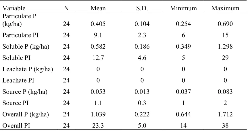
Table 2.2: Summary statistics of PLAT output in WFA method ...55

Table 2.3: Summary statistics of PLAT output in GA method...56

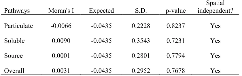
Table 2.4: Test of spatial autocorrelation in WFA method ...57

Table 2.5: Test of spatial autocorrelation in GA method ...58

Table 2.6: Test of data normality of PLAT outputs in each individual P loss pathway and at combined overall matter. Method used is Shapiro-Wilk test ...59

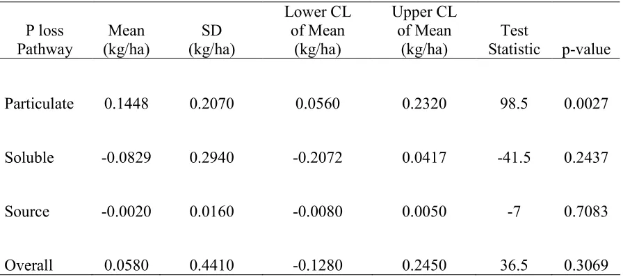
Table 2.7: Descriptive statistics and test of significance for the differences of P loss potential between two methods (GA-WFA) ...60

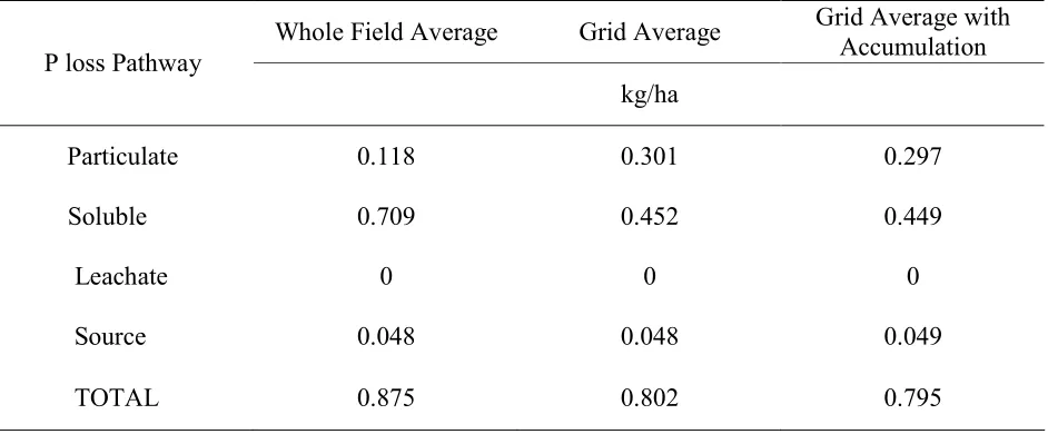
Table 2.8: Comparison of P loss potential from each pathway of PLAT modeling and test for P loss accumulation effect based on one field analysis...61

Chapter 3 Table 3.1: Moran’s I test of spatial autocorrelation ...91

Table 3.2: Shapiro-Wilk test of data normality for the difference of LS values from field measurement and GIS-based calculation...92

Table 3.3: Descriptive statistics and comparison of LS values estimated from GIS-aided RUSLE-based AML program and field measurements through whole field (WF) approach for test fields ...93

(10)

Table 3.5: Descriptive statistics and comparison of LS values estimated from GIS-aided RUSLE-based AML program and field measurements through

(11)

LIST OF FIGURES Chapter 1

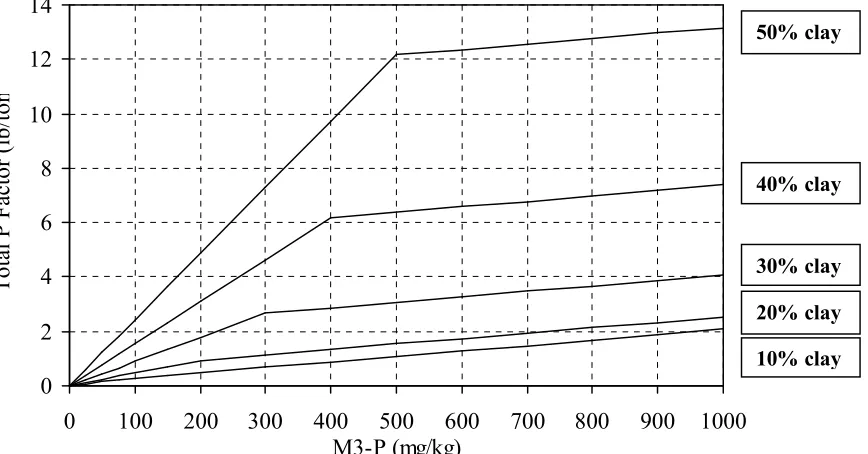
Fig. 1.1: Total P content of sediment as affected by clay content and M3-P. Lines represent example relationships. Inflection point represents threshold M3-P that results in 1 mg P/L solution P. (From PLAT model

description.) ...23

Fig. 1.2: Runoff P concentrations supported by soil groups as a function of M3-P (From PLAT model description.) ...24

Fig. 1.3: Leachate P concentrations as a function of M3-P levels at 30-in depth. (From PLAT model description.) ...25

Chapter 2 Fig. 2.1: Management zones and field boundaries of the study area map ...62

Fig. 2.2: Comparison of particulate P loss potential from PLAT by two methods: Whole Field Average (WFA) and Grid Average (GA) analysis...63

Fig. 2.3: Comparison of soluble P loss potential from PLAT by two methods: Whole Field Average analysis and Grid Average analysis...64

Fig. 2.4: Comparison of source P loss potential from PLAT by two methods: Whole Field Average analysis and Grid Average analysis...65

Fig. 2.5: Comparison of overall P loss potential from PLAT by two methods: Whole Field Average analysis and Grid Average analysis...66

Fig. 2.6: Comparison of particulate P loss through WFA and GA methods ...67

Fig. 2.7: Comparison of soluble P loss through WFA and GA methods ...68

(12)

Chapter 3

Fig. 3.1: (a). A conceptual 3 x 3 moving window explaining the position of the cells; (b). Scheme of assigning grid value for the flow direction derived

in ArcGIS. ...96 Fig 3.2: Whole average (WF) approach: comparisons of LS values from computer

estimates and those calculated from field measurements for test fields: slope cut-off factors of 0.7 for the fields with average slope > 5% and 0.5

for the fields with average slope ≤ 5%...97 Fig 3.3: Whole average (WF) approach: comparisons of LS values from computer

for the fields with average slope ≤ 5%...98 Fig 3.4: Whole average (WF) approach: comparisons of LS values from computer

for the fields with average slope ≤ 5%...99

Fig 3.5: Representative profile approach: comparisons of LS values from

computer estimates and those calculated from field measurements for test fields before and after adjustment: slope cut-off factors of 0.7 for the fields with average slope > 5% and 0.5 for the fields with average slope ≤

5% ...100 Fig 3.6: Representative profile approach: comparisons of LS values from

5% ...101 Fig 3.7: Representative profile approach: comparisons of LS values from

5% ...102 Fig. 3.8: Comparison of LS values calculated from field measurements and those

estimated from AML program through representative profile (RP)

approach with adjustment factor for validation fields: slope cut-off factors of 0.7 for the fields with average slope > 5% and 0.5 for the fields with

(13)

Fig. 3.9: Comparison of LS values calculated from field measurements and those estimated from AML program through representative profile (RP)

average slope ≤ 5% ...104 Fig. 3.10: Comparison of LS values calculated from field measurements and those

estimated from AML program through representative profile (RP)

(14)

CHAPTER 1

BACKGROUND AND LITERATURE REVIEW

THE PHOSPHORUS PROBLEM

Phosphorus (P) is a naturally occurring element that is vital to agricultural production and aquatic ecosystems. However, excessive agricultural source of P presents a potential risk to water quality (USEPA, 1996). In the U.S. and many other regions

around the world, P has contributed to non-point source pollution (NRC, 1992). The Clean Water Action Plan (USEPA-USDA, 1998) stated that “over-enrichment of waters by nutrients (nitrogen and phosphorus) is the biggest overall source of impairment of the nation’s rivers and streams, lakes and reservoirs, and estuaries.” The subsequent abiotic

and biotic disturbance following excessive P loading in water bodies include accelerated eutrophication (Fluck et al., 1992; Carpenter et al., 1998; Correll, 1998; Daniel et al., 1998; Glasgow and Burkholder, 2000), dissolved oxygen depletion (Rosa et al., 1987;

Axler et al., 1992; Bertram, 1993), toxic algal blooms (Paerl, 1988; Havens, 1994; Anderson et al., 2002), death of certain aquatic species (Ruello, 1976; Willemsen, 1980; Venugopalan et al., 1998; Jeppesen et al., 2002), and turbidity and bad odor (Sharpley et al., 1994). In the U.S, livestock and poultry manure are the key sources of excessive P.

The revised Clean Water Act implemented in 2003 forced the producers or growers of large concentrated animal feeding operations to obtain a permit under the National Pollution Discharge Elimination System (NPDES) regulations and apply manure based

(15)

Phosphorus sources

P comes from multiple sources, including organic byproducts, agricultural fertilizers, biosolids from municipal and industrial waste, and domestic wastewater. However, in agriculture, P mainly comes from the use of conventional commercial inorganic fertilizer,

and more dominantly animal waste, either spread as dry litter or sprayed as liquid waste (Edwards and Daniel, 1994; Williams et al., 1999). USDA-NRCS (1994) and USGS (1999) both identified agriculture P as a major contaminant of surface and ground water a

cropland-dominated watershed. Considerable research has been conducted to study the environmental impact of agricultural P (Daniel et al., 1998; Parry, 1998; Sims et al., 1998; Sharpley and Tunney, 2000). In North Carolina, the agricultural P problem is critical because of massively industrialized livestock production in the form of Confined Animal

Feedings Operations (CAFO), which is arguably a type of production that exceeds the assimilatory capacity for animal waste both locally and regionally that threatens downstream aquatic ecosystems (Austin, 1996; Sharpley, 1997; Martinez and Peu, 2000;

Novak et al., 2000). Crouse et al. (2001) showed that P applied through animal waste exceeded P requirements of all agronomic crops in, representing about 85% of CAFO in the state..

Phosphorus modeling at different scales

Models were often developed to estimate the P loss potential based on the understanding of environmental, hydrologic, physical and chemical factors controlling P movement. This has been agreed to be an efficient approach considering the time and

(16)

select the most effective best management practices (BMPs), and apply them to critical

source areas (CSA) where P loss potential is the most severe (Heathwaite et al., 2000; Weld et al., 2001; Sharpley et al., 2002; Page et al., 2005). Another advantage of modeling is the feasibility of prompt computer simulation under various hypothetical

management scenarios through an integrated approach. Total Maximum Daily Loads (TMDLs), which specifies the maximum amount of a pollutant that a water body can receive and still meet water quality standards, is legislated by USEPA in Section 303(d)

of the 1972 Clean Water Act. Phosphorus modeling, as part of the nutrient management plan, provides a reliable P loading estimate and thus serves as the basis of implementation of TMDLs and the evaluation of numerous management practices.

Popular process-based P loss assessment models include Agricultural Nonpoint

Source model (AGNPS, Young et al., 1989) and AnnAGNPS (Croshley and Theurer., 1998), Soil and Water Assessment Tool (SWAT, Arnold et al., 1998), Areal Nonpoint Source Watershed Environment Response Simulation (ANSWERS, Beasley et al., 1985;

Bouraoui and Dillaha, 1996), Guelph Model for Evaluating the Effects of Agricultural Management Systems on Erosion and Sedimentation (GAMES, Cook et al., 1985), Erosion-Productivity Impact Calculator (EPIC, Sharpley and Williams, 1990). In response to the revised USDA-NRCS Nutrient Management (590) Field Office Technical

Guide, the P index, together with agronomic soil test P interpretation and environmental soil test P threshold, are the three approaches that can be used to assess agricultural fields in P loss potential (USDA-NRCS, 1999).

(17)

the most efficient and robust approach because of the nature of site-specific assessment

of P delivery, and therefore has been widely adopted by 49† states, with appropriate modifications, to target P management (Sharpley et al., 2003). A P index tool can provide references for field staffs, watershed planners, and land users to assess the various

landforms and management practices for potential risk of P loading to water bodies (Sharpley et al., 2003).

Phosphorus reduction efforts

In addition to P loss modeling at the field, watershed and regional scale, several studies have been conducted to reduce the P loss by chemical approaches, including aluminum amendment into poultry litter (Hunger et al., 2004), immobilizing amendments for P sequestration (Zvomuya, 2006), use of dolomite phosphate rock (DPR) fertilizers to

reduce P leaching (Chen et al., 2006), and utilization of municipal and industrial wastes to reduce excessive bioavailable soil P (Peters and Basta, 1996). Typically engineering efforts include wetland and sediment trapping pond construction. Kao and Wu (2001)

found 59% of total P removal due to a mountainous natural wetland based on a major storm event study. Dunne et al. (2005) used soil/water column studies to determine the P release/retention rates. The study conducted by Liikanen et al. (2004) indicated that the processes taking place in the wetland diminished total P by 68% load and the dissolved

reactive P load by 49%. It is expected that the efficiencies of management practices, when combined with the identification of critical source areas through P loss assessment and modeling efforts, could considerably reduce P delivery to water bodies and thus

(18)

PHOSPHORUS LOSS ASSESSMENT TOOL OF NORTH CAROLINA In response to the revised USDA-NRCS nutrient management standard, 49states in the U.S. have adopted the P index method to develop their own P risk assessment tool (Sharpley et al., 2003). This is because the P index method considers individual P loss

pathways as affected by soil properties, climate, cropping system, management practices and other factors so that it can more comprehensively account for the between and within fields variations in P delivery potential compared with methods only using agronomic- or

environmental-based soil test P thresholds. North Carolina is one of the leading states in livestock and poultry production and historically animal waste has been applied based on crop nitrogen (N) requirement, which caused significant surplus P accumulation in agricultural soils (Crouse et al., 2001; N.C. Dept. Agric. Consumer Services, 2002).

Therefore, the Phosphorus Loss Assessment Tool (PLAT), a mechanistic model based on the P index concept was developed to evaluate the site-specific P loss potential from agricultural fields (The N.C. PLAT committee, 2005). PLAT rates the P loss potential

from a field based on P transport pathways, P source effects, and management factors. Specifically, PLAT takes into account the processes involved with P transport to surface and groundwater and evaluates the potential P risk in sediment-bound or particulate P, soluble P in surface runoff, soluble P in leaching water, and source effect on P loss.

Particulate P loss

Particulate P refers to P attached or adsorbed to soil particles transported with surface runoff into lakes, streams, and rivers during or after storms events (Daniel et al.,

(19)

major factors determining potential loss of particulate P include field erosion rate (ER,

tons/ac/yr) and P concentration in soil particles or total P factor (lbs/ton). PLAT considers the annual erosion rate from average sheet and rill erosion due to the action of water. Gully erosion is currently not included. The soil erosion rate is based on a reliable

estimated from the Revised Universal Soil Loss Equation (RUSLE) model (Wischmeier and Smith, 1965, 1978; USDA-NRCS, 1995; Renard et al., 1997). The parameter inputs for RUSLE include the rainfall erosivity factor (R, climate), soil erodibility factor (K,

soil), slope length (L) and slope steepness (S) factors (topography), cover management (C) and supporting conservation practices (P). The P concentration in the eroded soil particles is critical because it greatly influences the amount of total particulate P loss at a given soil erosion rate. The current implementation of PLAT relies on the Mehlich-3 P (M3-P)

soil test and average clay content to estimate the total P adsorbed to soil particles (Cox, 1994; Fig. 1.1). For North Carolina, the M3-P data (mg/kg) is converted from the Phosphorus Index (PI) value obtained from NCDA soil test information. The average

clay content (%) for the surface horizon (0-20 cm) of each soil map unit is available through the NRCSNational Map Unit Interpretation Record (MUIR) Database.

In addition to soil erosion rate and total P adsorbed, the net particulate P load to the nearby water bodies also depends on specific transport processes, during which P loss

may be reduced due to natural or anthropogenic causes. Therefore, the potential of soil erosion and particulate P loss from the source areas are usually higher than the actual amount of sediment yield and final P export. A typical natural factor PLAT considers is

(20)

relocates within the same field instead of being delivered beyond the field edge. On the

other hand, an enrichment factor is necessary to account for the increase of P concentration in fine-textured clay-enriched sediment due to particle selectivity during the deposition process (Wischmeier and Smith, 1978; Ongley, 1982; Foster et al., 1985).

The overall effect of receiving slope on the reduction of particulate P loss is represented in the edge of field delivery ratio (EFDR). There are also many examples of effective sediment-control and P-reduction practices, including vegetative or tree/shrub riparian

buffers (Peterjohn and Correll, 1984; Cooper and Gilliam, 1987; Daniels and Gilliam, 1996), sediment trapping ponds or basins (Bhaduri et al., 1995; Borden et al., 1998; Verstraeten and Poesen, 2002), as well as reduced tillage practices (Beasley et al., 1985; Gaynor and Findlay, 1995; Andraski et al., 2003). These optional practices, whether

implemented in the field or beyond the field edge, can often efficiently control soil erosion and sediment yield, and therefore reduce particulate P loss (Thaxton, 2005). In PLAT, these factors are represented by the buffer delivery ratio (BDR) and sediment trap

delivery ratio (STDR). In addition, PLAT also uses an Fe-P factor to account for the release of Fe-bound P as sediments are reduced in anaerobic environments (Shelton and Coleman, 1968). Other possible practices, but not evaluated in this component of PLAT, include crop rotation, contour cultivation, strip cropping, terraces, grass waterways, and

diversion structures.

After calculating soil erosion rate, total P adsorbed to sediment, and individual reduction factors, the equation for calculating particulate P loss is:

Particulate P Loss (lbs/ac) = ER (t/ac/yr) x Total P Factor (lbs P/ton) x EFDR

(21)

Soluble P loss

Soluble P represents the dissolved fraction of P in surface runoff water, which occurs when the precipitation rate exceeds the soil infiltration capacity. Soluble P exists

as orthophosphate, and can be readily taken up by aquatic plants and microorganisms. It is possible that soluble P is transformed into insoluble P through precipitation or adsorption as Al-P or Fe-P. Several researchers have concluded that drainage condition

can influence the amount and form of soluble P transport because the pipes and ditches provide further pathways of water flow and place outlets in addition to the gravitational water flux (Armstrong et al., 1984; Hawkins and Scholefield, 1996). The two major factors for estimating soluble P loss are runoff volume and P concentration in runoff

water. The release kinetics of both runoff and P concentrations are affected by several soil physical and chemical properties.

PLAT calculates the runoff volume differently for two situations, depending on

the drainage condition of the field. For moderately or excessively well drained fields with no artificially drainage, the USDA modified curve number approach is used to estimate the runoff potential (USDA-SCS, 1985). Inputs data needed for computing the curve

number include crop, qualitative hydrologic condition, and county-level long-term climate data. A runoff equation is developed for each county within North Carolina based on the long-term local weather data. For a field with a specific crop, soil, and hydrologic condition, the annual runoff is calculated from the exponential equation based on

determined curve number.

(22)

approach for estimating runoff volume. Input requirements for computing DI include

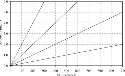
estimated drain depth, width between drains, and the soil map unit specific transmissivity value (Skaggs, 1980, 2004). The P concentration in the surface runoff is estimated as a function of M3-P soil test level (Fig. 1.2) (Pote et al., 1996; Liu et al., 1997; Sharpley

1997; Sims et al., 1998; McDowell et al., 2001a, b). PLAT classifies soils into four groups based on texture (organic, sands, loams, and clay soils), and the relationship between soluble P concentration and soil test P is developed for each soil texture group.

While the data are supported by substantial research when soluble P concentration is ≤ 1mg P/L, the relationship at > 1mg P/L are based on linear extrapolations that may underestimate soluble P and may need further field validation. (The N.C. PLAT Committee, 2005).

The practices that can effectively reduce particulate P loss, such as riparian buffers and receiving slopes, are not applicable to soluble P loss. However, some other practices that can reduce the runoff volume, such as conservation tillage or water control

structures, or that can decrease the soluble P concentration, such as microbial additives or addition of municipal and industrial wastes could mitigate soluble P loss to some degree (Peters and Basta, 2000; Zhu, 2006). For example, studies by Maguire et al. (2006) indicated that adding ≥ 10% CaO reduced the water-soluble P in manures by over 90%,

which greatly decreased soluble P loss potential. McGrath et al. (2005) and Maguire et al. (2004) also investigated the effect of dietary modification on P speciation in turkey and broiler litters and subsequent reduction in soluble P concentration. However, research on

(23)

Soluble P in Runoff (lb/ac/yr) = Runoff Concentration (mg/L)

x Runoff Volume (ac-in) / 4.415) [Eq. 1.2]

Subsurface P loss

Dissolved P may also be lost from agricultural fields by subsurface drainage or

leaching beyond the root zone. Significant P leaching usually occurs in sandy soils with moderately well to well drained hydrologic properties. However, some researchers also found considerable P leaching in clayey soils that exhibit substantial macropore water

flow (Djodjic et al., 1999; Laubel et al., 1999). Usually, soils with high M3-P level, shallow water table, and low P retention capacity have great potential of P leaching. Similarly with surface soluble P, the amount of P loss through subsurface transport depends on mainly two factors: the leachate water volume and the dissolved P

concentration. Skaggs et al. (2004) concluded that the relative proportions of water removed from poorly drained, high water table soils, as surface runoff, and through the profile as subsurface drainage, depend on precipitation, drain spacing and depth, soil

hydraulic properties, crop, and surface depressional storage. The formulas for estimating leachate volume depend on the drainage condition of the fields. For well-drained soils, the leachate volume is estimated from the mass balance of annual precipitation, runoff volume, and evapotranspiration (Eq. 1.3). While for poorly-drained soils with a high

water table, the average subsurface drainage is based on drainage intensity (DI) method from DRAINMOD model (Eq. 1.4).

Average subsurface drainage (in) = Annual PPT (in) – Runoff (in) – ET (in) [Eq. 1.3]

(24)

where DI is drainage intensity, and a, b, c,and d are regression coefficients characterized

by crop, location, and annual precipitation.

PLAT uses subsoil M3-P soil test (76 cm in depth) as an indicator of P loss through subsurface leaching. For soils with high P retention capacity in the upper soil

horizon, e.g., with high Fe and Al content, or soils with surface M3-P soil test (20 cm in depth) less than the threshold level of the corresponding soil group, leachate P concentration is treated as 0 mg/L. For soils with moderate or low P retention capacity,

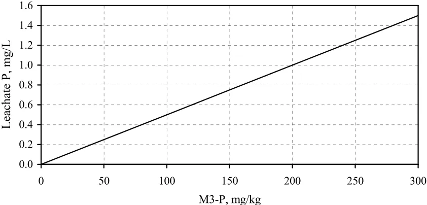
subsoil M3-P level is determined and the leachate P concentration is estimated through an empirical relationship (Fig. 1.3). When M3-P (76 cm) is > 50 mg/kg, which indicates the potential for P leaching, the P application rate is limited to crop removal.

Management practices to reduce leaching P loss are currently not considered in

version of PLAT, and equations 1.5 and 1.6 are used to calculate total leachate P loss for naturally drained soils and artificially drained soils, respectively.

Leachate P (lb/ac) = P concentration (mg/L)x [drainage volume (ac-in)/4.415] [Eq. 1.5]

Leachate P (lb/ac) = P concentration (mg/L)

x [drainage volume (ac-in)/4.415]x (T30 /TP) [Eq. 1.6] where, TP is the transmissivity of the entire profile and T30 is the transmissivity (12-30 in depth) that moves through the P-enriched soil zone (surface 30-in) and ultimately enters

the drainage system.

P in waste sources

Animal waste characteristics and management, together with soil properties,

(25)

concentration contained in different types of waste can vary greatly, such as 2.7 g P/L vs

1.2 g P/L in beef and dairy lagoon sludge, or 3.6 kg P/ton vs 17.3 kg P/ton in broiler fresh manure and house litter (Barker et al., 1994; USDA-NRCS, 1998; Dou et al., 2000; Sharpley and Moyer, 2000). Higher P loss through surface runoff would be expected if

animal waste is surface applied instead of incorporated or injected.

The waste source characteristics that influence P delivery to a surface water body are P application rate and total P content, P solids percentage, and soluble P content. Due

to high variability of manure composition, total P content largely depend on animal species, diet supplements, and type of waste handling and storage. The general trend of P content in common waste sources are poultry and turkey > beef > swine > dairy, and dry litter > liquid > slurry > sludge (Barker et al., 1994; Barnett, 1994; USDA-NRCS, 1998;

Dou et al., 2000; Sharpley and Moyer, 2000). Animal wastes with low percentage of solids, characterized by high water content, will have more dissolved P that can infiltrate into soils and reduce soluble P loss (Westerman et al., 1983). Waste sources with high

percentage of solids and low water content may contain low density waste particles that can float with water and increase P loss in surface runoff (Westerman et al., 1983).

In addition to waste source characteristics, application methods and timing also impact P loss. It has been well established that surface applications of animal wastes are

more subject to runoff loss than incorporation or injection (Mueller et al., 1984; Daniel et al., 1993). Tarkalson and Mikkelsen (2004) found that incorporation of broiler litter decreased flow-weighted concentration of reactive P in runoff by 97% and mass loss of

(26)

hours) resulted in significantly greater concentrations of dissolved P, bioavailable P,

particulate P, and total P (Eghball et al., 2002). Therefore, it is beneficial to avoid the periods with high probability of rainfall events when waste materials are surface applied.

Soluble and non-soluble P loss through surface runoff and subsurface drainage are

positively affected by rainfall intensity (Westerman et al., 1983). From previous studies, increased rainfall intensity caused elevated runoff volume but diluted P concentration, which may or may not result in increased amount of P loss (Edwards, and Daniel, 1993).

Therefore, a runoff fraction is used to estimate the maximum fraction of total mobile P that is surface transported. Specific effect of rainfall intensity on P transport varied with waste types and characteristics.

In PLAT, soluble P is calculated as the multiplication of total P and soluble

fraction, and non-soluble P is computed from P mass balance. PLAT estimates the total source P loss through soluble P and non-soluble P with corresponding adjustment factors (Eq. 1.7).

Total Source P loss = Soluble P x SPAF x RF x AF x AR

+ Non-soluble P x NSPAF x RF x BF x AF x AR [Eq. 1.7] where, SPAF is the soluble P attenuation fraction, NSPAF is the non-soluble P attenuation fraction RF is the runoff fraction, AF is the application fraction, and AR is the

application rate.

Overall P loss assessment rating

Although an individual P loss pathway is evaluated independently, interactions

(27)

(Baker and Johnson, 1976; Skaggs et al., 1982; Evans et al., 1995). Research by Vadas et

al. (2002) reported a 20 fold overprediction of P concentration in runoff compared with measured value, and the discrepancy was attributed to the possible resorption of P from the runoff solution by eroded sediment.

Although the interactions among individual P loss pathways occur, PLAT calculates the potential P loss from each pathway independently, and evaluates the overall P loss assessment as the mathematical summation of the estimates from all four

components (Eq. 1.8).. The equation for calculating the overall P loss is:

P Loss = Particulate P + Soluble P + Leachate P + Source P [Eq. 1.8]

This procedure generates a numerical value of potential P loss with the original unit of lbs P/ac/yr. PLAT as a P index tool, is not intended to represent the actual precise

quantity of P loss off a field (Lemunyon and Gilbert, 1993). Rather, PLAT is developed to make comparative estimate of relative risk of P loss potential under numerous site characteristics and management practices. Therefore, PLAT numerical outputs of each

field or management unit are converted into P loss index values and further classified into four qualitative categories. Each category is then assigned a relative P risk rating of “Low”, “Medium”, “High”, or “Very High”, which represents the relative field vulnerability to P loss. Based on the PLAT rating, a P management recommendation will

be proposed from no necessary adjustment to starter P application only (Table 1.1). PLAT links the waste source characteristics, P transport pathways, and management practices and eventually evaluates the risk of P loss on a site-specific basis.

(28)

identified aiding the selectivity and placement of efficient best management practices

(Weld et al., 2001; Page et al., 2005). In addition, once some management practices have been adopted, such as switching manure application method or building buffers beyond the field edge, PLAT can be used to assess the impact of these practices on reducing P

loss potential. Therefore, producers or growers can be protected and keep original agricultural production on non-critical source areas (Leytem et al., 2003).

SOIL EROSION AS AN ISSUE The problem and its process

Soil erosion caused by water, wind and anthropogenic activities such as tillage, deforestation, overgrazing, and construction is a global issue. USDA-NRCS (2000) calculated the combined water sheet and rill and wind erosion for the U.S. was 1.9 billion

tons in 1997. The overall erosion potential of a field or the spatial variability of erosion within a field is due to a combination of many factors, including the amount and the intensity of precipitation, soil type, topography, ground cover and land use. Generally

there are three types of soil erosion: mass movement (natural process due to gravity), water erosion, and wind erosion. There are two steps involved in the water erosion process: detachment and transport of soil particles. From a temporal standpoint, the erosion process is a sequence of events from raindrop splash to the convergence of gully

erosion. Therefore, water erosion can be further classified as splash erosion, sheet erosion, rill erosion, gully erosion, and tunnel erosion. It is necessary to understand the characteristics of each step in order to quantify soil erosion and propose appropriate

(29)

The adverse on-farm effect of erosion generates infertile soils and agricultural

production is significantly disturbed, which is especially critical for many developing countries where agriculture occupies the predominately proportion of the country’s economy. Currently, 97% of the world’s food supply comes from land with only 3%

coming from aquatic system. The topsoil, which contains the richest nutrient and organic matter for plant growth, is nearly irreplaceable, while it can be eroded in a short time period. Only when soil erosion is effectively controlled by proper farming and land

management practices and its adverse environmental impacts are minimized can agriculture be implemented in a sustainable matter.

Although soil erosion on U.S. cropland decreased 43% between 1982 and 2003 (NRCS, 2006), erosion is still the focus of many natural resource managers and soil

conservationists because of its off-farm impacts. The fraction of soil particles eroded that is finally delivered into water bodies represents non-point source pollution and negatively affects water turbidity in forms of either suspended particles or sediment (Uri, 2001). In

addition, sediment serves as the transporting vehicle of agchemicals such as pesticide and nutrients (especially P), which will impair water quality.

Quantification of soil erosion

Although precise quantification of soil erosion is still challenging (Dudal, 1982;

Lal, 1990), many field and lab studies have been conducted to calculate the overall soil erosion and sediment yield using radioactive 137Cs (Walling and Quine, 1990; Martz and Jong, 1991; Chappell et al., 1998; Collins et al., 2001). Another popular approach to

(30)

Martinez-Casasnovas, 2003; Mathys et al., 2003). The input data usually includes

climate, soil, terrain features, and land use. Soil erosion modeling, based on the understanding of soil detachment and transport process, is a convenient diagnostic tool and can provide reasonable estimates that support land use planning and effective

application of BMPs by resource managers and policy makers

The RUSLE (Revised Universal Soil Loss Equation) is a set of mathematical equations that estimate average annual soil loss and sediment yield resulting from interrill

and rill erosion. It is derived from the theory of erosion processes, supported by more than 10,000 plot-years of data from natural rainfall plots, and numerous rainfall-simulation plots. RUSLE is an exceptionally well-validated and documented equation. A strength of RUSLE is that it was developed by a group of nationally-recognized scientists

and soil conservationists who had considerable experience with erosional processes. RUSLE retains the structure of its predecessor, the USLE (Wischmeier and Smith 1965, 1978). WEPP (Water Erosion Prediction Project). It also includes simulation of

hydrologic and erosion processes at small watershed scales (Alberts et al., 1987; Laflen et al., 1987; Nearing et al., 1990; Laflen et al., 2004).

Another method, AGNPS (AGricultural Non-Point Source), is an event-based distributed parameter model developed by USDA-ARS for prediction of soil erosion and

sediment yield at the agricultural watersheds scale for real or hypothetical storms (Grunwald and Norton, 1999; Perrone and Madramootoo, 1999; Bhuyan et al., 2002). It was built upon the USLE algorithm but applied on a storm basis instead of annual

(31)

USPED (Unit Stream Power-based Erosion Deposition) is a simple model which

predicts the spatial distribution of erosion and deposition patterns and rates for steady state overland flow with uniform excessive rainfall conditions for sediment transport capacity. The model is based on the theory originally outlined by Moore and Burch

(1986) with numerous modifications (Mcisaac et al., 1992). One challenge for all these models is the generation of spatial and tabular parameters that can reflect the site characteristics the best possible yet not too memory-intensive and time-consuming to

cause computing problems. Scale issue as a spatial concern

Erosion potential and sediment yield have been studied at various spatial scales including plot (Wainwright et al., 2000; Bagarello and Ferro., 2004; Mathys et al., 2005;

Boix-Fayos et al., 2005; Parsons et al., 2006), field (Jetten et al., 1999; Barthes et al., 2000; Issa et al., 2006), watershed (Harden, 1992; Aksoy and Kavvas, 2005; Fu et al., 2005; Cohen et al., 2005), and national levels (Brazier et al., 2001). Currently there is no

universally successful method to transfer the soil erosion estimation algorithm or results between different scales. At the small scale (plot and field), environmental factors tend to be uniform, which reduces the difficulty of defining underlying erosion processes and, thus, improve the estimate accuracy. However, at large scales (watershed and national),

the environmental factors become complex and spatially heterogeneous, forcing the final algorithm, if feasible, to be limited to the study area from which it was developed or other similar sites with identical characteristics. As illustrated by Renard et al. (1997) and

(32)

measurement of soil loss. Some studies have been conducted to compare the performance

of different models at different scales (Amore et al., 2004; Reyes et al., 2004; Stolpe, 2005).

REVISED UNIVERSAL SOIL LOSS EQUATION MODELING

The Universal Soil Loss Equation (USLE) was first developed by Wischmeier and Smith and described in agricultural handbook (1965 and 1978). For many decades, USLE was the primary model used to assess soil loss potential in cropland at the field

scale through rill and interrill erosions and was used as a regulatory and conservation planning tool for government agencies in U.S. and many other countries. The Revised Universal Soil Loss Equation (RUSLE) is an upgrade of USLE that extends the application to mined lands, construction sites, and reclaimed lands.

As a one dimensional field-scale model, RULSE uses inputs of six factors that contribute to soil erosion. The basic equation is:

A = R * K * L * S * C * P [Eq. 1.8]

where, A is the average annual sheet and rill soil erosion in ton/ac-yr; The climate factor (R) is the rainfall erosivity, and is the product of rainfall energy and maximum 30-min intensity (EI30), often called Erosion Index. The soil factor (K) represents soil erodibility, or the soil loss rate per EI unit on a 22.13-m length and 9% standard fallow plot. The

slope length factor (L) is a dimensionless ratio of soil loss from the field slope length to that from a 22.13-meter plot under identical conditions. The slope steepness factor (S) is a dimensionless ratio of soil loss from the field slope to that from a 9% plot under

(33)

from an area with specified crop cover to that from an identical area in tilled continuous

fallow. The management factor (P) represents supporting practices, or the ratio of soil loss with a conservation practice to that with straight-row farming up and down slope. Among the factors, cover management is the most variable in that the type and amount of

surface residues and crop cover change during the year and between years. Natural events such as fire or human activities such as tillage can significantly increase the erosion rate. The type and intensity of vegetative cover greatly influences erosion rate through the

effects on aggregate stability and the control of runoff velocity. One source of error in the RUSLE estimate is the determination of the slope steepness (S) and slope length (L). Traditionally, these values come from field measurements by a specialist as described in the NRCS Field Technical Guide. As information technologies have evolved, many

researchers have been trying to estimate the soil erosion rate in an entirely digital environment based on the RUSLE algorithm combined with geospatial information (Hickey, 1994, 2000; Desmet and Govers, 1996; Dunn and Hickey, 1998; Van Remortel

et al., 2001).

Connections of P Loss and Soil Erosion

The studies of P loss and soil erosion are not isolated. Instead, soil loss is a very important component for estimating particulate P transported beyond the field edge as

sediment. Some models such as RULSE focus on soil loss potential, while other models such as Soil and Water Assessment Tool (SWAT) also consider the sediment delivery ratio (SDR) that calculates the sediment yield in a specified watershed. P loss models, as

(34)

and Theurer, 1998; Bhuyan et al., 2002). Recent research has been advanced in modeling

non-point source pollution which includes agricultural P and sediment yield at the watershed scale (Heathwaite et al., 2000; Weld et al., 2001; Sharpley et al., 2002; Fu et al., 2005). In PLAT, soil loss data on an annual basis comes from a RUSLE calculation

(35)

Table 1.1: PLAT overall rating of P loss potential and corresponding management recommendations

P Loss Estimate (kg/ha/yr)

P Loss Index

Ranking P Management Recommendation

0.0 to 1.1 0 - 25 Low No adjustment needed; N based application

>1.1 to 2.2 26 – 50 Medium No adjustment needed; N based application

>2.2 to 4.5 51-100 High Application limited to crop P removal

(36)

Fig. 1.1: Total P content of sediment as affected by clay content and M3-P. Lines represent example relationships. Inflection point represents threshold M3-P that results in 1 mg P/L solution P. (From PLAT model description.)

0 2 4 6 8 10 12 14

0 100 200 300 400 500 600 700 800 900 1000

M3-P (mg/kg)

T

o

ta

l

P

F

ac

to

r

(l

b

/t

o

n

)

50% clay

40% clay

30% clay

20% clay

(37)

Fig. 1.2: Runoff P concentrations supported by soil groups as a function of M3-P. (From PLAT model description.)

0.0 1.0 2.0 3.0 4.0 5.0 6.0

0 100 200 300 400 500 600 700 800 900 1000

M3-P (mg/kg)

S

o

lu

ti

o

n

P

(

m

g

/L

(38)

Fig. 1.3: Leachate P concentrations as a function of M3-P levels at 30-in depth. (From PLAT model description.)

0.0 0.2 0.4 0.6 0.8 1.0 1.2 1.4 1.6

0 50 100 150 200 250 300

M3-P, mg/kg

L

ea

ch

at

e

P

,

m

g

(39)

Literature Cited

Aksoy, H., and M.L. Kavvas. 2005. A review of hillslope and watershed scale erosion and sediment transport models. Catena. 64:247-271.

Alberts, E.E., C.S. Holzhey, L.T. West, and J.O. Nordin. 1987. Soil Selection: USDA water erosion prediction project (WEPP). Paper No. 87-2542, Am. Soc. Agric. Eng., St. Joseph, MI.

Amore E., C. Modica, M.A. Nearing, and V.C. Santoro. 2004. Scale effect in USLE and WEPP application for soil erosion computation from three Sicilian basins. J. Hydrol. 293:100-114.

Anderson, D.M., P.M. Glibert, and J.M. Burkholder. 2002. Harmful Algal Blooms and Eutrophication: Nutrient Sources, Composition, and Consequences. Estuaries. 25:704-726.

Andraski T.W., L.G. Bundy, and K.C. Kilian. 2003. Manure history and long-term tillage effects on soil properties and phosphorus losses in runoff. J. Environ. Qual. 32:1782-1789 Armstrong A.C., J.L. Atkinson, and E.A. Garwood. 1984. Grassland Drainage Economics Experiment, North Wyke, Devon. Ministry of Agriculture, Fisheries and Food, London. Arnold, J.G., R. Srinivasa, R.S. Muttiah, and J.R. Williams. 1998. Large area hydrologic modeling and assessment Part 1: Model development. J. Am. Water Resour. Assoc. 34: 73-89.

Austin, N.R., J.B. Prendergrast, and M.D. Collins. 1996. Phosphorus losses in irrigation runoff from fertilize red pasture. J. Environ. Qual. 25:63-68.

Axler, R., C. Larsen, C. Tikkanen, and M. McDonald. 1992. Water quality changes in mine pit lakes used for salmonid aquaculture. Aquaculture '92, Orlando, FL, May 21-25. Bagarello, V., and V. Ferro. 2004. Plot-scale measurement of soil erosion at the experimental area of Sparacia (southern Italy). Hydrol. Process. 18:141-157.

Baker, J.L., and H.P. Johnson. 1976. Impact of subsurface drainage on water quality. IN: Drainage for Increased Crop Production and a Quality Environment. Proc. Third National Drainage Symp. ASAE. Chicago, IL. p. 91-98.

(40)

Barthes, B., A. Azontonde, B.Z. Boli, C. Prat, and E. Roose. 2000. Field-scale run-off and erosion in relation to topsoil aggregate stability in three tropical regions (Benin, Cameroon, Mexico). Eur. J. Soil Sci. 51:485-495.

Beasley D.B, E.J. Monke, E.R. Miller, and L.F. Huggins. 1985. Using simulation to assess the impacts of conservation tillage on movement of sediment and phosphorus into Lake Erie. J. Soil Water Conserv. 40:233-237.

Bertram, P.E. 1993. Total Phosphorus and Dissolved Oxygen Trends in the Central Basin of Lake Erie, 1970-1991. J. Gt. Lakes Res. 19:224-236.

Bhaduri, B.L., J.M. Harbor, and P.A. Maurice. 1995. Chemical Trap Efficiency of a Construction Site Storm-Water Retention Basin. Physical Geol. 16:389-401.

Bhuyan S.J., L.J. Marzen, J.K. Koelliker, J.A. Harrington, and P.L. Barnes. 2002. Assessment of runoff and sediment yield using remote sensing, GIS, and AGNPS. J. Soil Water Conserv. 57:351-364.

Boix-Fayos, C., M. Martinez-Mena, E. Arnau-Rosalen, A. Calvo-Cases, V. Castillo, and J. Albaladejo. 2006. Measuring soil erosion by field plots: Understanding the sources of variation. Earth-Sci. Rev. 78:267-285.

Borden, R.C., J.L. Dorn, J.B. Stillman, and S.K. Liehr. 1998. Effect of In-Lake Water Quality on Pollutant Removal in Two Ponds. J. Environ. Engineering. 124:737-743. Bouraoui F., and T.A. Dillaha. 1996. ANSWERS-2000: Runoff and sediment transport model. J. Environ. Eng. 122:493-502.

Brazier R.E., J.S. Rowan, S.G. Anthony, and P.F. Quinn. 2001. "MIRSED" towards an MIR approach to modelling hillslope soil erosion at the national scale. Catena. 42:59-79. Carpenter S.R., N.F. Caraco, D.L. Correll, R.W. Howarth, A. N. Sharpley, and V.H. Smith. 1998. Nonpoint pollution of surface waters with phosphorus and nitrogen. Ecol. Appl. 8:559-568.

Chappell A., A. Warren, M. A. Oliver, and M. Charlton. 1998. The utility of 137Cs for measuring soil redistribution rates in southwest Niger. Geoderma. 81:313–337.

Chen G.C., Z.L. He, P.J. Stoffella, X.E. Yang, S. Yu, and D. Calvert. 2006. Use of dolomite phosphate rock (DPR) fertilizers to reduce phosphorusleaching from sandy soil Environ. Pollut. 139:176-182.

(41)

Collins A.L., D.E. Walling, H.M. Sichingabula, and G.J.L. Leeks. 2001. Using (CS)-C-137 measurements to quantify soil erosion and redistribution rates for areas under different land use in the Upper Kaleya River basin, southern Zambia. Geoderma. 104:299-323.

Cook D.J., W.T. Dickinson, and R.P. Rudra. 1985. GAMES—The Guelph Model for Evaluating the Effects of Agricultural Management Systems on Erosion and Sedimentation. User’s Manual. Technical Report 126-71. Guelph, Ontario: School of Engineering, University of Guelph.

Cooper, J.R., and J.W. Gilliam. 1987. Phosphorus redistribution from cultivated fields into riparian areas. Soil Sci. Soc. Am. J. 51:1600-1604.

Correll, D. L. 1998. The role of phosphorus in the eutrophication of receiving waters: A review. J. Environ. Qual. 27:261-266.

Cox, F.R. 1994. Predicting increases in extractable phosphorus from fertilizing soils of varying clay content. Soil Sci. Soc. Am. J. 58:1249-1253.

Croshley R.G., and F.G. Theurer. 1998. ANAGNPS Non Point Pollutant Loading Model: Proceedings of the First Federal Interagency Hydrologic Modeling Conference. Las Vegas, Nevada. 19-23.

Crouse D.A., R.E. Austin, S.C. Hodges, and J.C. Barker. 2001. North Carolina Nutrient Management Database Project. Available: http://www.soil.ncsu.edu/nmp/

Daniel D.C., D.R. Edward, and A.N. Sharpley. 1993. Effect of Extractable soil surface phosphorus on runoff water quality. Trans. Am. Soc. Agric. Eng. 36:1079-1085.

Daniel T.C., A.N. Sharpley, D.R. Edwards, R. Wedepohl, and J.L. Lemunyon. 1994. Minimizing surface water eutrophication from agriculture by phosphorus management. J. Soil Water Conserv. 49:30–38.

Daniel T.C., A.N. Sharpley, and J.L. Lemunyon. 1998. Agricultural phosphorus and eutrophication: A symposium overview. J. Environ. Qual. 27:251–257.

Daniels, R.B., and J.W. Gilliam. 1996. Sediment and chemical load reduction by grass and riparian filters. Soil Sci.Soc. Amer. J. 60:246-251.

Desmet P.J.J., and G. Govers. 1996. A GIS procedure for automatically calculating the USLE LS factor on topographically complex landscape units. J. Soil Water Conserv. 51: 427-433.

(42)

Dou, Z., J.D. Toth, D.T. Galligan, C.F. Ramberg, and J.D. Ferguson. 2000. Laboratory procedures for characterizing manure phosphorus. J Environ. Qual. 29:508-514. Drever, J. L. The Geochemistry of Natural Waters. Prentice: New Jersey. 1997:87-90. Dudal R. 1982. Land degradation in a world perspective. J. Soil Water Conserv. 37:245-249.

Dunn M., and Hickey R. 1998. The effect of slope algorithms on slope estimates within a GIS. Cartography. 27(1): 9-15.

Dunne E.J., N. Culleton, G. O'Donovan, R. Harrington, and K. Daly. 2005. Phosphorus retention and sorption by constructed wetland soils in Southeast Ireland. Water Res. 39:4355-4362.

Edwards, D.R., and T.C. Daniel. 1993a. Effects of poultry litter application rate and rainfall intensity on quality of runoff from fescuegrass plots. J.Envir. Qual. 22:361-365. Edward, D.R., and T.C. Daniel. 1993b. Runoff quality impacts of swine manure applied to fescue plots. Trans. Am. Soc. Agric. Eng. 36:81-86.

Edwards, D.R., and Daniel T.C. 1994. Quality of runoff from fescuegrass plots treated with poultry litter and inorganic fertilizer. J. Environ. Qual. 23:579-584.

Eghball, B., J.E. Gilley, D.D. Baltensperger, and J.M. Blumenthal. 2002. Long-term manure and fertilizer application effects on phosphorus and nitrogen in runoff. Trans. ASAE. 45:687-694.

Evans, R.O., R.W. Skaggs, and J.W. Gilliam. 1995. Controlled versus conventional drainage effects on water quality. J. Irr. & Drain. Eng. ASCE. Special Issue July/August. p.271-276.

Fluck R.C., C. Fonyo, and E. Flaig. 1992. Land-use-based phosphorus balances for Lake Okeechobee, Florida, drainage basins.Appl. Eng. Agric. 8: 813–820.

Foster G., and S. Dabney. 1995. ‘Agricultural Tillage Systems: Water Erosion and Sedimentation’, Farming for a Better Environment, Soil and Water Conservation Society, Ankeny, IA.

Fu B.J., W.W. Zhao, L.D. Chen, Q.J. Zhang, Y.H. Lu, H. Gulinck, and J. Poesen. 2005. Assessment of soil erosion at large watershed scale using RUSLE and GIS: A case study in the Loess Plateau of China. Land Degrad. Dev. 16:73-85.

(43)

Glasgow H.B., and J.M. Burkholder. 2000. Water quality trends and management implications from a five-year study of a eutrophic estuary. Ecol. Appl. 10:1024-1046. Grunwald S., L.D. Norton. 1999. An AGNPS-based runoff and sediment yield model for two small watersheds in Germany. Trans. ASAE. 42:1723-1731.

Hansen N.C., A.N. Daniel, A.N. Sharpley, and J.L. Lemunyon. 2002. The fate and transport of phosphorus in agricultural systems. J. Soil Water Conserv. 57:409-417. Harden C.P. 1992. Incorporating roads and footpaths in watershed-scale hydrologic and soil-erosion models. Phys. Geogr. 13:368-385.

Havens, K.E. 1994. Relationship of annual chlorophyll a means, maxima, and algal bloom frequencies in a shallow eutrophic lake (Lake Okeechobee, Florida, U.S.A.). Lake Reserv. Manag.10:133–138.

Haygarth P.M., P.J. Chapman, S.C. Jarvis, and R.V. Smith. 1998. Phosphorus budgets for two contrasting grassland farming systems in the UK. Soil Use Manage. 14:160-167. Hawkins J.M.B, and D. Scholefield. 1996. Molybdate-reactive phosphorus losses in surface and drainage waters from permanent grassland. J. Environ. Qual. 25:727-732.

Heathwaite L., A. Sharpley, and W. Gburek. 2000. A conceptual approach for integrating phosphorus and nitrogen management at watershed scales. Conference on Practical and Innovative Measures for the Control of Agricultural Phosphorus Losses to Water, Antrim, Northern Ireland. 29:158-166.

Hickey R., A. Smith, and P. Jankowski. 1994. Slope length calculations from a DEM within ARC/INFO GRID. Comput. Environ. Urban. 18:365-380.

Hickey R. 2000. Slope Angle and Slope Length Solutions for GIS. Cartography. 29:1-8. Hunger S., H. Cho, J.T. Sims, and D.L. Spark. 2004. Direct speciation of phosphorus in alum-amended poultry litter: Solid-state [31] P NMR investigation. Environ. Sci. Technol. 38:674-681.

Issa O.M., Y. Le Bissonnais, O. Planchon, D. Favis-Mortlock, N. Silvera, and I. Wainwright. 2006. Soil detachment and transport on field- and laboratory-scale interrill areas: erosion processes and the size-selectivity of eroded sediment. Earth Surf. Process. Landf. 31:929-939.

(44)

Jetten V, A. de Roo, and D. Favis-Mortlock. 1999. Evaluation of field-scale and catchment-scale soil erosion models. Catena. 37:521-541.

Kao C.M., and M.J. Wu. 2001. Control of non-point source pollution by a natural wetland. Water Sci. Technol. 43:169-174.

Khaleel, R., K.R. Reddy, and M.R. Overcash. 1980. Transport of potential pollutants in runoff water from land areas receiving animal wastes: a review. Water Research. 14:421-436.

Khan N.I., and Islam A. 2003. Quantification of erosion patterns in the Brahmaputra-Jamuna River using geographical information system and remote sensing techniques. Hydrol. Process. 17:959-966.

Laflen J. M., A.W. Thomas, and R. Welch. 1987. Cropland experiments for the WEPP project. Paper No. 87-2544, Am. Soc. Agric. Eng., St. Joseph, MI.

Laflen J.M., D.C. Flanagan, and B.A. Engel. 2004. Soil erosion and sediment yield prediction accuracy using WEPP. J. Am. Water Resour. Assoc. 40:289-297.

Lal R., and B.A. Stewart. 1990. Soil Degradation. New York, Springer-Verlag.

Laubel, A., O.H. Jacobsen, B. Kronvang, R. Grant, and H.E. Andersen. 1999. Subsurface drainage loss of particles and phosphorus from filed plot experiments and tile-drained catchment. J. Environ. Qual. 28:76-584.

Lemunyon, J.L., and R.G. Gilbert. 1993. The concept and need for a phosphorus assessment tool. J. Prod. Agric. 6:483-486

Leytem, A.B., J.T. Sims, and F.J. Coale. 2003. On-farm evaluation of a phosphorus site index for Delaware. J. Soil Water Conserv. 58:89-97

Liikanen A, M. Puustinen, J. Koskiaho, T. Vaisanen, P. Martikainen, H. Hartikainen. 2004. Phosphorus removal in a wetland constructed on former arable land. J. Environ. Qual. 33: 1124-1132.

Liu F., C.C. Mitchell, D.T. Hill, J.W. Odom, and E.W. Rochester. 1997. Phosphorus recovery in surface runoff swine lagoon effluent by overland flow. J. Environ. Qual. 26:995-1001.

(45)

Maguire R.O., J.T. Sims, W.W. Saylor, B.L. Turner, R. Angel, T.J. and Applegate. 2004. Influence of phytase addition to poultry diets on phosphorus forms and solubility in litters and amended soils. J. Environ. Qual. 33:2306-2316

Mallin M.A., L.B. Cahoon. 2003. Industrialized animal production - A major source of nutrient and microbial pollution to aquatic ecosystems. Popul. Environ. 24:369-385. Martinez J., and P. Peu. 2000. Nutrient fluxes from a soil treatment process for pig slurry. Soil Use Manage. 16:100-107.

Martinez-Casasnovas J.A. 2003. A spatial information technology approach for the mapping and quantification of gully erosion. Catena. 50:293-308.

Martz L.W. and E. Jong. 1991. Using cesium-137 and landform classification to develop a net soil erosion budget for a small Canadian prairie watershed. Catena. 18:289–308. Mathys N., S. Brochot, M. Meunier, and D. Richard. 2003. Erosion quantification in the small marly experimental catchments of Draix (Alpes de Haute Provence, France). Calibration of the ETC rainfall-runoff-erosion model. Catena. 50:527-548.

Mathys N., S. Klotz, M. Esteves, L. Descroix, J.M. Lapetite. 2005. Runoff and erosion in the Black Marls of the French Alps: Observations and measurements at the plot scale. Catena. 63: 261-281.

McDowell R., A. Sharpley, P. Brookes, and P. Poulton. 2001a. Relationship between soil test phosphorus and phosphorus release to solution. Soil Sci. 166:137-149.

McDowell R.W., A.N. Sharpley, L.M. Condron,, P.M. Haygarth, and P.C. Brookes. 2001b. Process controlling soil phosphorus release to runoff and implication for agricultural management. Nutr. Cyl. Agroecosyst. 59:269-284.

McGrath J.M., J.T. Sims, R.O. Maguire, W.W. Saylor, C.R. Angel, and B.L. Turner 2005. Broiler diet modification and litter storage: Impacts on phosphorus in litters, soils, and runoff. J. Environ. Qual. 34:1896-1909

Mcisaac G.F., J.K. Mitchell, J.W. Hummel, and W.J. Elliot. 1992. An evaluation of unit stream power theory for estimating soil detachment and sediment discharge from tilled soils. Trans. ASAE. 35:535-544.

Moore I.D., and G.J. Burch. 1986. Sediment transport capacity of sheet and rill flow: application of unit stream power theory. Water Resour. Res. 22:1350-1360.

(46)

Nair V.D., and D.A. Graetz. 2004. Agroforestry as an approach to minimizing nutrient loss from heavily fertilized soils: the Florida experience. Agrofor. Syst. 61-2:269-279. National Research Council. 1992. Restoration of aquatic ecosystems. National Academy Press, Washington, D.C. Natural Resource Conservation Service. 2006. Annual National Resources Inventory 2003. Raleigh, NC.

Nearing M.A., L.M. Risse, J.M. Laflen, and. J.E. Ferris. 1990. WEPP hillslope erosion model predictions for natural runoff plots. Am. Soc. Ag. Eng. Paper 90-2078. ASAE Summer Meeting, Columbus, OH. June 24-27.

North Carolina Department of Agriculture. and Consumer Services. Agricultural Statistics Division. 2002. http://www.ncagr.com/stats/index.htm.

Novak J.M., D.W. Watts, P.G. Hunt, and K.C. Stone. 2000. Phosphorus movement through a coastal plain soil after a decade of intensive swine manure application. J. Environ. Qual. 29: 1310-1315.

Ongley, E.D. 1982. Influence of season, source and distance on physical and chemical properties of suspended sediment. Recent Developments in the Explanation and Prediction of Erosion and Sediment Yield. IAHS Publ. No.137:371-383.

Paerl, H.W. 1988. Nuisance phytoplankton blooms in coastal, estuarine and inland waters. Limnol. Oceanogr. 33:823–847.

Page T., P.M. Haygarth, K.J. Beven, A. Joynes, T. Butler, C. Keeler, J. Freer, P.N. Owens, and G.A. Wood. 2005. Spatial variability of Soil Phosphorus in Relation to the Topographic Index and Critical Source Areas: Sampling for Assessing Risk to Water Quality. J. Environ. Qual. 34:2263-2277.

Parry R. 1998. Agricultural phosphorus and water quality: A U.S. Environmental Protection Agency perspective. J. Environ. Qual. 27:258-261.

Parsons A.J., R.E. Brazier, J. Wainwright, and D.M. Powell. 2006. Scale relationships in hillslope runoff and erosion. Earth Surf. Process. Landf. 31:1384-1393.

Perrone J., and C.A. Madramootoo. 1999. Sediment yield prediction using AGNPS. J. Soil Water Conserv. 54 :415-419.

Peterjohn, W.T., and D.L. Correll. 1984. Nutrient dynamics in an agricultural watershed: Observations on the role of a riparian forest. Ecology. 65:1466-1475.