Scholarship at UWindsor
Scholarship at UWindsor
Electronic Theses and Dissertations Theses, Dissertations, and Major Papers
2012
Damage and material identification using inverse analysis
Damage and material identification using inverse analysis
Li Li
University of Windsor
Follow this and additional works at: https://scholar.uwindsor.ca/etd
Recommended Citation Recommended Citation
Li, Li, "Damage and material identification using inverse analysis " (2012). Electronic Theses and Dissertations. 4825.
https://scholar.uwindsor.ca/etd/4825
This online database contains the full-text of PhD dissertations and Masters’ theses of University of Windsor students from 1954 forward. These documents are made available for personal study and research purposes only, in accordance with the Canadian Copyright Act and the Creative Commons license—CC BY-NC-ND (Attribution, Non-Commercial, No Derivative Works). Under this license, works must always be attributed to the copyright holder (original author), cannot be used for any commercial purposes, and may not be altered. Any other use would require the permission of the copyright holder. Students may inquire about withdrawing their dissertation and/or thesis from this database. For additional inquiries, please contact the repository administrator via email
DAMAGE AND MATERIAL IDENTIFICATION USING INVERSE ANALYSIS
by
Li Li
A Dissertation
Submitted to the Faculty of Graduate Studies
through Department of Civil and Environmental Engineering in Partial Fulfillment of the Requirements for
the Degree of Doctor of Philosophy at the University of Windsor
Windsor, Ontario, Canada
2012
DAMAGE AND MATERIAL IDENTIFICATION USING INVERSE ANALYSIS
BY
Li Li
APPROVED BY:
______________________________________________ R. Ben Mrad, External Examiner
University of Toronto
______________________________________________ N. Zamani
Department of Mechanical, Automotive & Materials Engineering
______________________________________________ B. Budkowska
Department of Civil & Environmental Engineering
______________________________________________ S. Cheng
Department of Civil and Environmental Engineering
______________________________________________ F. Ghrib, Advisor
Department of Civil and Environmental Engineering
______________________________________________ J. Albanese, Chair of Defense
Department of Sociology, Anthropology & Criminology
DECLARATION OF ORIGINALITY
I hereby certify that I am the sole author of this thesis and that no part of this thesis has
been published or submitted for publication.
I certify that, to the best of my knowledge, my thesis does not infringe upon
anyone‘s copyright nor violate any proprietary rights and that any ideas, techniques,
quotations, or any other material from the work of other people included in my thesis,
published or otherwise, are fully acknowledged in accordance with the standard
referencing practices. Furthermore, to the extent that I have included copyrighted
material that surpasses the bounds of fair dealing within the meaning of the Canada
Copyright Act, I certify that I have obtained a written permission from the copyright
owner(s) to include such material(s) in my thesis and have included copies of such
copyright clearances to my appendix.
I declare that this is a true copy of my thesis, including any final revisions, as
approved by my thesis committee and the Graduate Studies office, and that this thesis has
ABSTRACT
In this thesis, we formulate novel solutions to two inverse problems using optical
measurements as input data: i) local level damage identification of beams, and ii) material
constitutive parameter identification using digital image correlation measurement of
surface strain/displacements.
A novel photogrammetric procedure based on edge-detection was devised to
measure the quasi-continuous deflection of beams under given loading. This method is
based on the close-range photogrammetry technique made possible through recent
developments of image processing algorithms and modern digital cameras.
Two computational procedures to reconstruct the stiffness distribution and to
detect damage in Euler-Bernoulli beams are developed in this thesis. The first
formulation is based on the principle of the equilibrium gap along with a finite element
discretization. The solution is obtained by minimizing a regularized functional using a
Tikhonov Total Variation (TTV) scheme. The second proposed formulation is a
minimization of a data discrepancy functional between measured and model-based
deflections. The optimal solution is obtained using a gradient-based minimization
algorithm and the adjoint method to calculate the Jacobian. The proposed identification
methodology is validated using experimental data. The proposed methodology has the
potential to be used for long term health monitoring and damage assessment of civil
engineering structures.
The identification of material plasticity parameters is carried out by minimizing a
least-square functional measuring the gap between inhomogeneous displacement fields
identified simultaneously by means of direct, derivative-free optimization methods where
the finite element simulation is treated as a black-box procedure. Methods verifying and
validating the identified results are given. Particular interest is given to the identifiability
issue in deterministic and statistical sense. The validation procedure intends to detect
false positive results (type-II errors). The performance of the computational procedures
is illustrated by numerical and experimental examples. The proposed approach avoids
using the gradient of the cost function in the identification process; it has the benefit of
ACKNOWLEDGEMENTS
First, I would like to express my sincere gratitude to my advisor Dr. F. Ghrib for his
patient instructions, insightful comments and financial assistance during the research
program. I also would like to thank my committee members, Dr. Zamani, Dr.
Budkowska, and Dr. Cheng, for their valuable suggestions to improve this thesis. I owe
much thanks to Dr. W. Altenhof, Dr. H.K. Kwan, for their teaching during my training at
the University of Windsor. My deep appreciation and gratitude goes to Dr. Green of the
department of Mechanical Engineering for providing me the ARAMIS optical testing
system. I would like to thank the technical staff in the Civil and Mechanical Engineering
Laboratories, to their assistance during the test programs. I would also like to recognize
individually, friends and staff in the University of Windsor: Catherine Wilson, Lucian
Pop, Pat Seguin, Andrew Jenner, Matt St. Louis, Wafa Polies; their help and support
TABLE OF CONTENTS
DECLARATION OF ORIGINALITY ... iii
ABSTRACT ... iv
ACKNOWLEDGEMENTS ... vi
LIST OF TABLES ...x
LIST OF FIGURES AND ILLUSTRATIONS... xii
LIST OF SYMBOLS, ABBREVIATIONS AND NOMENCLATURE ...xv
CHAPTER ONE: INTRODUCTION ...1
1.1 General ...1
1.2 Optical full-field measurements using digital cameras ...4
1.3 Damage identification based on static tests ...5
1.4 Material parameter identification using full-field measurements ...6
1.5 Hyperelasticity model parameter identification for rubber and rubber-like solids ....8
CHAPTER TWO: OPTICAL MEASUREMENT USING DIGITAL CAMERAS: DIGITAL IMAGE CORRELATION AND CLOSE-RANGE PHOTOGRAMMETRY ...9
2.1 Introduction ...9
2.2 Close-range photogrammetry and applications in civil engineering ...10
2.2.1 Overview ...10
2.2.2 Applications of close-range photogrammetry in civil engineering ...24
2.3 Close-range photogrammetry for beam deflection measurement ...26
2.3.1 Overview ...26
2.4 Photogrammetric measurement of beam deflection using an edge-based approach ...30
2.5 Photogrammetric measurement of beam deflection using a surface-based approach ...40
2.6 Digital image correlation ...40
2.7 Summary ...45
CHAPTER THREE: DAMAGE IDENTIFICATION OF EULER-BERNOULLI BEAMS USING FULL-FIELD MEASUREMENTS ...46
3.1 Introduction and background ...46
3.1.1 An introduction to damage identification problem ...46
3.1.2 Material-level methods ...47
3.1.3 System identification ...48
3.1.4 Model updating ...49
3.1.5 Finite element model updating ...50
3.1.6 The four levels of damage assessment ...50
3.1.7 Classification of damage identification methods ...51
3.1.8 Overview of this chapter ...53
3.2.1 Dynamic damage identifications ...54
3.2.2 Static response data-based damage identification ...60
3.2.3 Advantages and disadvantaged of static and dynamic identifications ...68
3.3 Equilibrium gap method ...72
3.4 Data discrepancy-based FE model updating ...80
3.5 Examples ...85
3.5.1 Numerical examples ...85
3.5.1.1 Validation of the Equilibrium Gap Method ...85
3.5.1.2 Validation of the Data Discrepancy Functional Method ...87
3.5.2 Experimental examples ...90
3.5.2.1 Test # 1: Step-wise damage detection ...91
3.5.2.2 Test # 2: Single saw-cut damaged beam ...94
3.5.2.3 Test # 3: Discrete three saw-cuts damaged beam ...96
3.5.2.4 Test #4: Combination of discrete and step cuts damaged beam ...98
3.6 Conclusions ...104
3.7 Extension and envision: ...105
CHAPTER FOUR: MATERIAL PARAMETER IDENTIFICATION USING FULL-FIELD MEASUREMENTS ...107
4.1 Introduction and literature review of related research ...107
4.1.1 General review ...107
4.1.2 Outline of the proposed methodology ...111
4.1.3 The advantages of using DIC ...113
4.1.4 Organization of this chapter ...115
4.2 Overview of elasto-plasticity ...116
4.3 General methodology ...118
4.4 Nonlinear regression theory: parameter estimation using statistical inference ...120
4.5 Least-squares formulation and solution of the identification problem ...122
4.6 Overview and selection of optimization techniques ...127
4.7 Statistical inference with DIC data ...136
4.7.1 Nonlinear regression inference using linear approximation ...137
4.7.2 Calculation of Sensitivity ...140
4.7.3 Checking response fit ...141
4.8 Identifiability issues ...142
4.8.1 General ...142
4.8.2 Ill-posed or well-posed ...143
4.8.3 Model and parameter identifiability ...144
4.8.4 Verification and validation (V&V) ...144
4.8.5 Quality and nature of information from data ...146
4.8.6 Curvature measure of nonlinearity: checking the adequacy of linearized covariance analysis (LCA) ...148
4.8.7 Summary of procedures addressing the identifiability issue ...152
4.9 Examples and results ...154
4.9.1 Numerical example ...154
4.10 Summary of this study ...175
CHAPTER FIVE: HYPERELASTICITY MODEL IDENTIFICATION FOR RUBBER AND RUBBER-LIKE SOLIDS ...177
5.1 Introduction and literature review of related research ...177
5.2 Hyperelastic models for rubber-like materials ...185
5.3 Methodological and analytical approaches used for this project ...192
5.4 Results and illustrative examples ...193
5.4.1 Rubber block ...193
5.4.2 Engine mount ...195
5.5 Summary ...205
CHAPTER SIX: CONCLUSION AND FUTURE WORK ...207
REFERENCES ...209
LIST OF TABLES
Table 3.1: A synopsis for the classification of damage identification methods ... 53
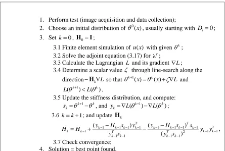
Table 3.2: Damage identification algorithm using the adjoint-optimization method. ... 84
Table 3.3: Identified stiffness of test #1 ... 101
Table 3.4: Identified stiffness of test #2 ... 102
Table 3.5: Identified stiffness of test #3 ... 103
Table 3.6: Identified stiffness of test #4 ... 103
Table 4.1: identified solution with and without synthetic noise (load factor = 1.1) ... 157
Table 4.2: Comparison of identification solution with and without synthetic noise to Nelder-Mead and Genetic Algorithm (GA) methods (load factor = 1.1) ... 158
Table 4.3: Identification solution without synthetic noise (load factor = 1.05) IM=0.0001 ... 159
Table 4.4: identification solution without synthetic noise (load factor = 1.1)(Tresca yield criterion) IM= 0.0002 ... 160
Table 4.5: Re-identified parameters with and without synthetic noise ... 168
Table-4.6: Parameter identification with Stage 10 measurement data (elastic response)171 Table-4.7: Identification with Stage 50 data ... 172
Table 5.1: Popular constitutive models for compressible rubberlike materials in FE analysis ... 191
Table 5.2: numerical test of the inverse problem (IM = 0.0001) ... 194
Table 5.3: numerical test of the inverse problem with 5% synthetic noise (IM = 0.0004) ... 195
Table 5.4: numerical test of the inverse problem using simulated surface displacements (IM = 0.0006) ... 199
Table 5.5: numerical test of the inverse problem using simulated surface displacements with synthetic noise (IM = 0.0013) ... 200
LIST OF FIGURES AND ILLUSTRATIONS
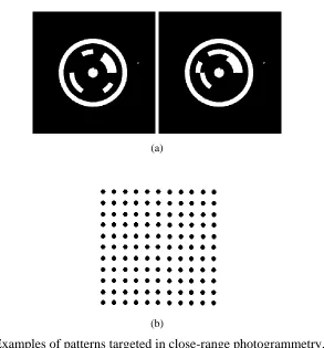
Figure 2.1: Examples of patterns targeted in close-range photogrammetry. a) Targets attached to the surface and used for measuring displacements of concrete beams (Niederöst and Maas, 1997); and b) a dense grid of circles printed on the surface of testing structures (Cardenas-Garcia, Wu et al., 1997) (Hegger, Sherif et al., 2004) (Franke, Franke et al., 2007). ... 12
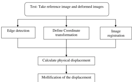
Figure 2.2: Procedural steps for beam deflection measurement using photogrammetry based on edge-detection. ... 31
Figure 2.3. The laboratory set-up for tests of a step-cut beam. ... 32
Figure 2.4. The detected upper-edge of a cantilever beam: a) a cut-out RGB image; b) the detected edge in a grey-scale image; and c) a binary image of the edge
generated using a pixel threshold. ... 33
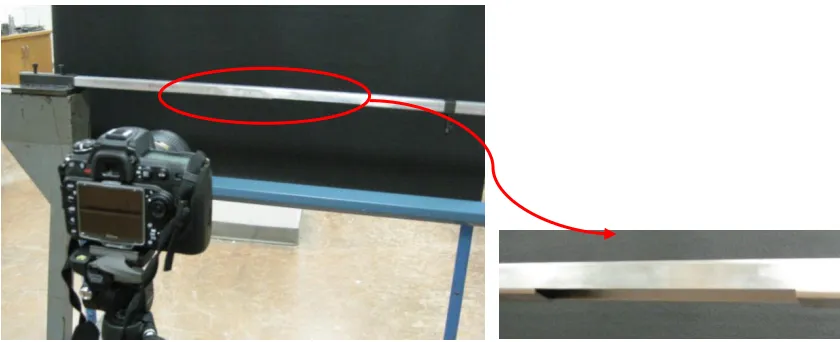
Figure 2.5: The experimental set-up for close-range photogrammetric measurement of the displacement of a loaded cantilever beam with a high-contrast stable
background using consumer-grade optical equipment. ... 38
Figure 2.6: Beam deflection: Experimentally-obtained measurements using
edge-detection methods and close-range photogrammetry technique. ... 39
Figure 2.7: Beam Deflection: Theoretical deflections with E = 66 GPa and E = 72 GPa, and correspondence of the predicted values to the experimentally-measured deflection profile shown in the previous figure. Predictions were based on elastic beam theory. The elasticity modulus of the aluminum alloy material was calibrated at 70.14 GPa. Measurements were obtained using edge-detection
methods and close-range photogrammetry techniques. ... 39
Figure 2.8: Rotation computation from the mollified displacement measurements. ... 40
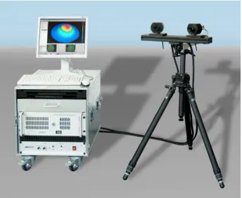
Figure 2.9: the ARAMIS system of the GOM Company ... 44
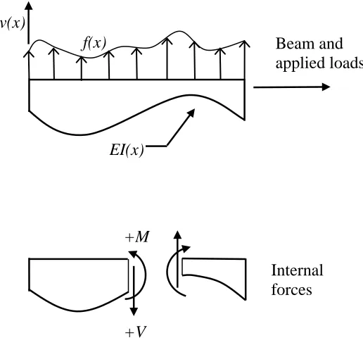
Figure 3.1: Internal force equillibrium in Euler-Bernoulli beams subjected to flexure. ... 74
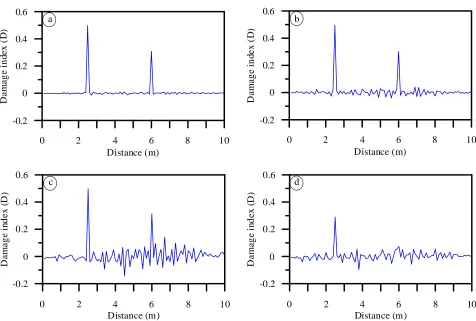
Figure 3.2: Identified damage indices of a simply-supported beam using the
equilibrium gap method. (a): no noise, (b): 2.5% noise, (c): 5% noise, (d): 10% noise. ... 87
Figure 3.4: Identified stiffness factor distribution for a simply-supported beam with constant stiffness using the data discrepancy functional method ... 89
Figure 3.5: Identified stiffness factor distribution for a simply-supported beam with parabolic stiffness variation. ... 90
Figure 3.6. The cantilever beam with a distributed damage. ... 91
Figure 3.7. Damage detection of the cantilever beam with distributed damage using the equilibrium gap method. ... 92
Figure 3.8. Identified stiffness factor distribution of the cantilever beam with
distributed damage using the data discrepancy formulation. ... 92
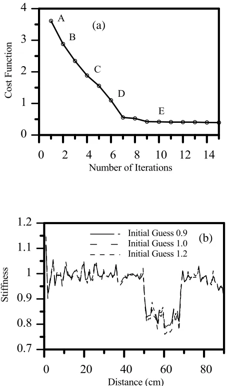
Figure 3.9. Performance of the adjoint based method for solving the data discrepancy problem, (a) convergence rate, (b) influence of the initial guess, (c) iteration
process for initial guess EI0 and (d) iteration process for intial guess 1.2 EI0. ... 94 Figure 3.10: Uniform cantilever beam with a saw-cut damage ... 95
Figure 3.11: Damage detection of saw-cut beam using the equilibrium gap method ... 96
Figure 3.12: Identified stiffness factor distribution of the saw-cut beam using the data discrepancy formulation. ... 96
Figure 3.13. The cantilever beam with three saw-cuts damage. ... 97
Figure 3.14. Damage detection of the beam with three saw-cuts using the equilibrium gap method. ... 98
Figure 3.15. Identified stiffness factor distribution of the beam with three saw-cuts using the data discrepancy formulation. ... 98
Figure 3.16. Cantilever beam with double saw-cuts and a distributed damage. ... 99
Figure 3.17. Damage detection of the beam with saw-cuts and step damage using the equilibrium gap method. ... 100
Figure 3.18. Identified stiffness factor distribution of the beam with saw-cuts and step damage using the data discrepancy formulation. ... 100
Figure 4.1: Flowchart of material parameter identification using optimization-based FE-model updating ... 119
Figure 4.2: Plate with a hole under tension ... 155
Figure 4.4: the bearing cap ... 162
Figure 4.5: photo of the bearing cap on the testing machine and two cameras taking images ... 163
Figure 4.6: FE model of the bearing cap... 163
Figure 4.7: Horizontal strain μx simulated by the FE model ... 164
Figure 4.8: typical stress-strain curves for cast iron materials under tension and compression ... 165
Figure 4.9: a bilinear approximation model for cast iron material ... 165
Figure 4.10: typical images from a DIC test result in ARAMIS; data measured inside the red rectangle are used in the identification pocess ... 166
Figure 4.11: the sensitivity of the identification of one parameter E. (Left: the sensitivity surface of identified E with respect to the errors in the x- and y-translation; Right: sensitivity of the surface of the objective function with respect to the errors in the x- and y- translation) ... 173
Figure 4.12: the sensitivity of the identification of four parameters Et, Ec, ϵt, ϵcand the objective function. ... 174
Figure 5.1: The simulated strain contours of a rubber block using COMSOL ... 193
Figure 5.2: The engine mount and the DIC test using the ARAMIS DIC system ... 197
Figure 5.3: The geometry model and finite element model of the engine mount ... 198
Figure 5.4: The DIC measurements of displacement in the 7.8 kN load case ... 202
Figure 5.5: The FE simulation of displacement at the 7.8 kN load case using identified Mooney-Rivlin model ... 202
LIST OF SYMBOLS, ABBREVIATIONS AND NOMENCLATURE
Abbreviations Definition
CONDOR COnstrained, Non-linear, Direct, parallel Optimization using trust Region method for high-computing load function
DFO Derivative-Free Optimization
DIC Digital Image Correlation
DOF Degree Of Freedom
FEM Finite Element Method
FRF Frequency Response Function
LCA Linearized Covariance Analysis
LS Least-Squares
RSM Response Surface Methodology
TV Tikhonov-Total Variation
VFM Virtual Fields Method
V&V Verification and Validation
Symbols Definitions
B The left Cauchy-Green tensor
C The right Cauchy-Green tensor
𝒅 Test data set
𝐸 Modulus of elasticity
𝒇 Force vector in FEA
𝑓(𝑥) A function
F Deformation gradient
𝑮 System matrix in the equilibrium gap method 𝐼𝑀 The relative offset measure
𝐽 Objective function to be minimized
𝐽𝛿𝑓(𝑥) Mollifier of function 𝑓(𝑥) 𝑱 𝜽 Jacobian evaluated at 𝜽
𝑲, 𝒌𝑖 Stiffness matrix and element stiffness matrix in FEA
𝑷 Covariance matrix
T The first Piola-Kirchhoff stress tensor
𝒖 Displacement vector
𝑣 Deflection of a beam
𝑊 The strain energy function
𝒙 Coordinates
𝛼 Tikhonov regularization parameter
𝛿 The mollifier‘s radius
Φ 𝛉 The regularization function
𝜃 Rotation angle of a beam
𝜽, 𝜃𝑖 Parameter vector and its components
Ω A region or a subset
𝝈 Cauchy stress
CHAPTER ONE: INTRODUCTION
“The mere formulation of a problem is far more essential than its solution, which may be merely a matter of mathematical or experimental skills. To raise new questions, new possibilities, to regard old problems from a new angle require creative imagination and marks real advances in science.” Albert Einstein
1.1 General
Traditional techniques in experimental mechanics rely on displacement or strain
transducers carefully placed in a small number of positions on the surface of the tested
specimen. The data usually consist of series of test data correlated with the applied load
and the measured field (usually a displacement or strain component). The recent
development of new technologies combining low-cost CCD cameras and computer vision
led to novel experimental methods to assess solids and structures. Non-contact
measurement techniques are now becoming affordable for research and development
purposes in laboratories as well as for on-site monitoring of structures.
Digital image correlation (DIC), moiré and speckle interferometry, and grid
methods are among the many new technologies that can be utilized in the field of
experimental mechanics. The fundamental shift in the possibilities offered by these new
technologies is related to the spatial properties of the collected data. For example, a
typical DIC test system commonly has the capability of collecting up to 10,000
independent displacement measurements from the surface of the specimen. The large
not be possible using traditional transducers. For example, in the context of constitutive
laws identification, the geometry and the boundary conditions must be very simple when
traditional transducers are used, so that an analytical solution of the stress/strain field is
possible; the stress and strain fields must be homogeneous in order to determine the
material properties. Consequently, the identification of constitutive laws requires more
than one test, since only the mechanical properties associated with the mechanisms
activated during the test can be identified. When non-contact measurement techniques
are used along with the finite element method (FEM), however, the need for simplified
loading and boundary conditions is relaxed. Non-contact measurement techniques with a
single test set-up can replace the large number of test set-ups involving various
combinations of experimental parameters that are necessary when local transducers are
used.
Full-field displacement measurements allow much greater flexibility as they
provide very rich experimental data and allow the use of tests under non-homogeneous
conditions. However, the large amount of data produced by full-field measurement
techniques requires suitable computational methods to extract the information
encapsulated within the non-homogeneous displacement and strain fields. The effort to
integrate new measurement technologies in experimental mechanics has introduced a
completely new research area, referred to as inverse problems in solid mechanics.
Full-field displacement measurements can also be integrated with numerical
simulation techniques such as FEM to build health monitoring systems for structures in
service. The methodology consists of incorporating the measured displacement or strain
location and severity of damage. The formulation of a health monitoring problem as an
inverse problem has become a very important subject that has attracted a great deal of
interest and research activity over the last decade.
This thesis concerns two aspects of research based on the use of full-field
measurement techniques and finite element simulations for the health monitoring of
structures and for constitutive law identification. In the first part of this work, we
formulate the problem of reconstruction of the stiffness of beams through the
measurement of displacements along the beam. In the second part of this thesis, we study
the implementation of this material identification problem using DIC to measure the
displacement and strain on the surface of a specimen.
Each of these issues is of the utmost importance in practice. Currently, there is an
increasing demand for effective methods to identify complex nonlinear material models.
The competitive industrial environment leads engineers to develop better, but also more
complex models of complicated systems. These models are generally difficult to define,
and the work presented here is a step towards the development of a systematic approach
for material characterisation. Furthermore, the problem of reconstruction of a beam‘s
stiffness can be considered as one of the fundamental problems in the health monitoring
of these important structural elements.
From a mathematical point of view, the problems mentioned above can be
considered as two examples of inverse problems. However, the stiffness reconstruction
of beams is typically classified as an ill-posed functional identification problem, whereas
the identification of material properties is considered a well-posed parameter
evaluating the response of the studied structure to a known force or displacement where
the basic parameters, such as the geometry of the structure and the mechanical properties
of the materials, are known. Inverse problems, on the other hand, seek to determine
unknown geometrical and/or mechanical parameters from the known measured responses
of the system.
A direct procedure can rarely compute material and geometric properties from
measurable responses, such as displacements or strains. Inverse methods usually
formulate the problem as a minimization of error function between measured and
computed responses; this is also called an estimation function. These inverse procedures
usually involve finite-element (FE) model-updating techniques.
1.2 Optical full-field measurements using digital cameras
The damage identification methods developed in this thesis require a technique to
measure the displacements during static loading tests. In optical measurements, objects
are measured without being touched. A novel procedure based on edge-detection was
devised to measure the quasi-continuous deflection of beams under given loading, and is
presented in Chapter 2. This method is based on the close-range photogrammetry
technique made possible through recent developments of image processing algorithms
and modern digital cameras. These studies demonstrate that modern consumer cameras
can be used in optical measurement procedures, offering an additional advantage in terms
of cost.
The studies of material parameter identification presented in this thesis employ
3D components as input for the inverse analysis. DIC is an image analysis technique
based on grey-value digital images that can determine the contour and the displacements
of an object under load in three dimensions with sub-pixel precision. This technique is
already mature and commercialized; Chapter 2 provides a brief description of the DIC
technique, and the commercial DIC system employed in the current work.
1.3 Damage identification based on static tests
The problem of stiffness reconstruction is presented in Chapter 3. In this chapter,
we are particularly interested in formulating the identification of damage from static
measurement. Static tests are the most direct way of evaluating the load-bearing capacity
of structures. All structures throughout their service undergo a continual and ongoing
accumulation of damage and decreased loading capacity. Consequently, damage
identification is an important aspect of safety and functionality, and has attracted
intensive research efforts over the past twenty years.
Two computational procedures using static deflection measurements to
reconstruct the stiffness distribution, and to detect regions containing damages in
Euler-Bernoulli beams, are presented and compared in Chapter 3. The first proposed
formulation is based on the principle of the equilibrium gap along with a FE
discretization, and the mathematical problem leads to an over-determinate linear system.
The solution is obtained by minimizing a regularized function with a Tikhonov Total
Variation (TTV) regularization scheme. The second proposed formulation is defined as a
minimization of a data discrepancy functional between measured and model-based
algorithm and the adjoint method to calculate the Jacobian. The two proposed
methodologies are validated using experimental data.
1.4 Material parameter identification using full-field measurements
Modern design and performance evaluation requires realistic simulations of
structural and material behaviour, and nonlinear FE simulation has become a fundamental
engineering tool. FE approaches are increasingly popular among engineers from
different industries. Constitutive parameters associated with nonlinear models are not
always available in standard material databases; therefore, engineers need to identify
them experimentally.
Although the identification of plasticity material parameters is the focus of the
current work (presented in Chapter 4), this study aims to provide a unified identification
methodology. In light of recent developments in direct optimization and regression
analysis, particularly the verification and validation of the material parameter
identification using statistical tools, this thesis proposes novel procedures for the
identification of material parameters in any given model.
The problem of material parameter identification is formulated as a nonlinear
regression problem using DIC measurement data as the input. The study presented in
Chapter 4 includes the following topics: definition of the inverse problem; a brief
description of the derivative-free optimization scheme; discussion of the identifiability
issues related to the inverse approach; and the application of statistical inference with a
Solution of the material parameter identification problem was performed by
minimizing a least-squares (LS) function measuring the gap between inhomogeneous
displacement fields obtained from DIC measurements and FE simulations. Specifically,
a LS formulation of a cost function consisting of a norm for the discrepancies between
the experimental data and the simulated data was minimized; the simulated data was
obtained by the FE method using commercial software. Direct, derivative-free
optimization methods, which treat the FE simulation as a black-box procedure, identified
the material parameters simultaneously. Particular attention was paid to the
identifiability and numerical stability issues of this approach, and methods for verifying
and validating the identified results are discussed. In particular, consideration is given to
the identifiability issue in the deterministic and the statistical sense. Sampling-based
statistical inference derived from nonlinear regression theory was adopted to quantify the
quality of the identification procedure, the rationale being that DIC provides a large
amount of data, and thus allows the use of statistical inference. Sampling-based
inference and sensitivity analysis were used to check the adequacy of the identification
solution, thus avoiding Type-2 errors (i.e., the acceptance of incorrect results). Several
recommended numerical approaches for validating the identification results are presented.
Linearized covariance analysis (LCA) was adopted to check the fit of the parameters. An
index derived from the response surface geometry was used to check the response fit, and
relative curvature measures proposed to check the adequacy of LCA. The proposed
validation procedure is primarily intended to detect false positives (i.e., Type-II errors).
The proposed approach avoids using the gradient of the cost function in the
box to solve the direct problem. The quantification of the quality of the result is of
paramount importance to the practical application of any identification methodology.
1.5 Hyperelasticity model parameter identification for rubber and rubber-like solids
The mechanical behaviour of rubber-like materials is usually characterized by a
strain energy density function 𝑊; the parameters of the 𝑊 function may be considered as
material parameters. Traditional laboratory techniques require several tests — using
different homogeneous deformation modes and standard cut-out samples — to determine
the appropriate strain energy form and parameters.
The general approach for material parameter identification (described in Chapter
4) was used to determine the parameters of strain energy functions (𝑊) with DIC test
data collected for the original structural components. In this approach, whole field
displacement/strain on the surface of components is measured by a DIC-based technique,
which provides massive amounts of experimental data in a single test. The DIC-based
methodology for parameter identification in hyperelasticity models (presented in Chapter
5) replaces the performance of multiple tests on simple-shape specimens with supposed
CHAPTER TWO: OPTICAL MEASUREMENT USING DIGITAL CAMERAS: DIGITAL IMAGE CORRELATION AND CLOSE-RANGE PHOTOGRAMMETRY
“It is necessary to measure everything that can be measured and to try making measurable what isn’t as yet.” Galileo
2.1 Introduction
The technique of obtaining information from photographs is called photogrammetry. The
most important feature of photogrammetry is that objects are measured without being
touched. The development of photogrammetry has a long history, particularly the branch
related to aerial photogrammetry. Currently, with the development of computer and
digital photography, photogrammetric technology has changed dramatically from purely
optical equipment to fully digital workflow (i.e. without any type of film or plotter), and a
new branch — close-range photogrammetry, also termed vision metrology or
videogrammetry, is developing rapidly. Furthermore, inexpensive digital consumer
cameras have reached a high technical standard with good geometric resolution, and can
replace expensive metric cameras for close-range photogrammetry as long as the
accuracy/precision required for the measurement is not too high (Linder, 2009).
While close-range photogrammetry is used primarily for field measurements, the
application of optical measurements in an experimental setting has aroused interest. For
example, holographic interferometry, moiré and moiré interferometry, and speckle
innovation, digital image correlation (DIC), developed in the 1980s is now
commercialized for use in industrial processes.
Close-range photogrammetry and DIC developed independently from each other.
Nevertheless, DIC can be regarded as a branch of close-range photogrammetry. The
research presented in this thesis uses digital cameras to optically measure beam deflection
profiles and full-field displacements/strains on the surface of specimens and components
for inverse identification processes. This chapter briefly reviews some of the concepts
and procedures involved in close-range photogrammetry and its application to civil
engineering. Two novel techniques proposed for the measurement of beam deflection
profiles in a laboratory setting are presented: 1) an based technique using
edge-detection suitable for beams with a clean surface and smooth edges; and 2) a
surface-based technique using image correlation. Finally, DIC methods are briefly described.
The novel methods are presented in the following sections: Section 2 describes
the new approach: edge-based deflection measurement of beams is introduced with
example. The data of this example is served as the input to the new damage
identification method to be introduced in Chapter 3. In Section 3, the fundamental theory
and characteristics of DIC measurement is described. Beam deflection measurement
using image correlation is presented in Section 5, with example of a concrete beam.
2.2 Close-range photogrammetry and applications in civil engineering
2.2.1Overview
The primary purpose of a photogrammetric measurement, both aerial and
and derived geometric elements). For every image point, values in the form of
radiometric data (intensity, grey value, and color value) and geometric data (position in
image) can be obtained.
Close-range photogrammetry differs from traditional far-field photogrammetry
and image-based measurement systems as the primary task in close-range
photogrammetry is to measure the three-dimensional coordinates of targets placed on all
areas of interest on a structure or system, whereas the primary tasks in traditional
photogrammetry and image-based measurements are feature extraction, object
identification, and metrological measurement at relatively lower accuracy (Heijden,
1994). Thus, the key to the technique of close-range photogrammetry is the precise
calculation of the positions of each of the targets in the field of view; see (Luhmann,
Robson et al., 2006) for an overview of traditional methods and models in close-range
photogrammetry.
Laser-scanning measurement is an alternative to photogrammetry. The advantage
of laser-scanning methods is that the object can be low-textured while photogrammetric
techniques often require highly textured objects. On the other hand, laser-scanning
techniques are time-consuming and usually very expensive.
Visible patterns are a very important feature of photogrammetry, particularly
patterns that can be identified using pixel or color information. Patterns targeted in
close-range photogrammetry are usually simply attached metallic stickers. Popular types of
surface patterns targeted in photogrammetry are illustrated in Figure 1 and may include:
metallic targets attached to the surface; and 4) small, color printed circles attached to the
surface.
(a)
(b)
Figure 2.1: Examples of patterns targeted in close-range photogrammetry. a) Targets attached to the surface and used for measuring displacements of concrete beams (Niederöst and Maas, 1997); and b) a dense grid of circles printed on the surface of
testing structures (Cardenas-Garcia, Wu et al., 1997) (Hegger, Sherif et al., 2004) (Franke, Franke et al., 2007).
Traditional close-range photogrammetry is applied to objects ranging from 1 m to
200 m in size; the level of accuracy depends on the distance between the camera and the
object, and the size of the area to be measured. Typically, accuracy ranges from <0.1mm
for smaller areas to 1 cm for larger areas (Luhmann, Robson et al., 2006; Linder, 2009).
Digital image processing (DIP) techniques such as image correlation, image registration,
General information related to: a) basic procedures; b) digital images; c) image
coordinate systems and orientation; and d) reference or control points are briefly
summarized in the following pages.
Close-range photogrammetric measurement procedures
The fundamental procedures of a close-range photogrammetric measurement
include the preparation and recording of images, pre-processing, orientation calculations,
measurement, and image analysis. The steps in the general protocol for close-range
photogrammetry can be summarized as follows:
1. Preparation and recording of images
a) Application of surface targets.
b) Determination of control points or scaling lengths.
c) Image recording.
2. Pre-processing
a) Computation: calculate reference point coordinates and/or distances
from survey observations.
3. Orientation and measurement calculation
a) Measurement of image points: identification and measurement of
reference and scale points, including tie points (points observed in
multiple images).
b) Bundle adjustment: simultaneously calculate both interior and exterior
orientation parameters as well as the object point coordinates required
for subsequent analysis.
4. Measurement and analysis
a) Single point measurement: identify the pixel coordinates of each point
to be measured in the image, and transform to physical coordinates.
b) Calculate displacements.
c) Field measurement: with interpolation and smoothing, measured points
can be connected and interpolated to make a field measurement.
Specific experimental procedures for the research presented in this thesis are
described in later sections. Some general concepts related to the composition of digital
images, image coordinate systems and the use of reference points to establish their
relationship to object coordinates (orientation), and digital imaging systems are
introduced in the following pages.
Digital images:
The essential advantage in using digital images over traditional photos is the ease
in image-processing, such as image enhancement, deblurring, edge-sharpening and
de-noising, thus attains the maximal utilization of information contained in images. The
digital image is actually a rectangular array composed of picture elements called pixels.
Each pixel is assigned an intensity value meant to characterize the color of a small
rectangular segment of the scene. A high-resolution picture can contain 5 to 10 million
pixels, while a low-resolution picture small picture may contain comparatively few pixels
(e.g. 256 × 256 = 65536 pixels). Digital image processing is thus notorious for its
intensive computation.
Grey-scale images are typically recorded by means of a charge-coupled device
the amount, or intensity, of the light that hits each detector. Thus, we can think of a
grey-scale image as a rectangular 𝑚 × 𝑛 array with entries that represent light intensities.
A digital image may be considered as a matrix made up of elements that are
positive integers representing surface brightness. Each of these elements is called a pixel,
which has a specific value in a range that depends on the digital camera and the image
acquisition electronics (e.g. for an 8-bit system, there are 256 grey values ranging from
0-255). Measurements, such as the 2D in-plane incremental displacement field, can be
assessed by comparing successive digital images. Generally, grey-scale images of this
type are used in image processing for edge detection, image registration, and image
correlation.
Metric cameras are monochrome; using a monochrome camera has several
advantages over a digital camera with Red–Green–Blue (RGB) color sensor. A
monochrome sensor has no color filter in front of the sensor. This increases the
International Organization for Standardization (ISO) rating of the sensor to 200 as
compared to ISO 80 for the color version of the same sensor. All pixels are sensitive to
the same spectrum of light. The information at each pixel location is not interpolated on
a monochrome sensor. Pixels of a typical RGB color sensor are arranged in a one layer
matrix of which 50%, 25%, and 25% are masked green, red, and blue, respectively.
During post-processing this single layer of pixels is interpolated to a triplet of layers,
meaning that 50%, 75%, and 75% of the pixels representing the green, red, and blue
channels of the image, respectively, must be interpolated from pixels with a different
color. This interpolation can lead to artefacts in the images, reducing the geometric
one image to 18 MB for a sensor with 6 million pixels and 8 Bit color depth, as compared
to a monochrome image, while no information is added. Image correlation software
typically employs only one color channel of an image for analysis (ERDAS, 2002). This
implies that 100% of the original information of a monochrome sensor can be utilized by
the software while a single layer of a colour image will carry at most only 50% of the
original resolution of an RGB sensor. At the same time, image file size is reduced and
light sensitivity of the sensor is increased when using a monochrome camera. An image
size of 6MB allowed analysis to be performed on uncompressed Tagged Image File
Format (TIFF) images. The image compression in JPEG format may bring more blurring
and loss of information (Li, Yuan et al., 2002).
However, consumer cameras typically use color sensors. Color images in the
RGB format can be separated into three grey-scale images or matrices; one of these can
then be used for image processing. Alternatively, one can calculate a mixed
monochrome image matrix using the following well-known formula (Linder, 2009):
grey value = 0.3 × red(R) + 0.11 × green(G) + 0.59 × blue(B)
Generally, this calculation can be easily performed with image-processing
software by activating the option ―mixed image‖ when importing images (Linder, 2009;
Umbaugh, 2011).
World and camera coordinates
In measuring the position and orientation of objects with computer vision
methods, we have to couple the coordinates of the camera system (coordinates of the
The coordinates of the camera system are denoted 𝒙 = 𝑥, 𝑦, 𝑧 𝑇. Usually the 𝑧
axis is aligned with the optical axis orthogonal to the image plane. The world coordinates
are denoted as 𝑿 = [𝑋, 𝑌, 𝑍] . The two coordinates are coupled by two linear
transformations: a translation and a rotation. The translation is a shift of origin and can
be described with a vector 𝒕. If the two origins coincide, the remaining differences can
be neutralized by rotations. Here, we have also three degrees of freedom: 𝜙, 𝜓, and 𝜃.
Mathematically, rotation corresponds to multiplication of the coordinate vector with a
3 × 3 orthogonal matrix 𝑹. Clearly, the matrix depends nonlinearly on the three rotation
parameters. As a whole, the coupling between world coordinates and camera coordinates
is given by the following expression: 𝒙 = 𝑹(𝑿 − 𝒕), i.e. the ideal imaging process is a
linear transformation between world coordinates/object points and sensor/image
locations. However, there are potential for distortions when using this ideal pinhole
model to predict image locations.
Pin-hole camera model
Perspective projection is a simple model describing the image formation with a
lens system; it is equivalent to a pinhole camera model (Heijden, 1994). Such a model
consists of a non-transparent plane with a small hole. Parallel to this plane, at a distance
𝑑, the image plane is located. Light emitted from the surfaces of objects in the scene
passes through the hole and illuminates the image plane. If the pinhole is small enough,
an infinitesimal small surface patch of an object is mapped onto a small spot of light at
the image plane. The collection of all surface patches will give rise to an irradiance
called image. In the pinhole model, each point in the image plane corresponds exactly to
The pinhole camera model is based on the principle of collinearity, where each
point in the object space is projected by a straight line through the projection center into
the image plane. Usually, the pinhole model is a basis that is extended with some
corrections for the systematically distorted image coordinates. The most commonly used
correction is for the radial lens distortion that causes the actual image point to be
displaced radially in the image plane.
Image coordinate system (pixel coordinate system) and orientation
In principle, the one-to-one correspondence between the physical and image
coordinates of the object has to be established via a camera/lens calibration procedure.
The image coordinate system described above is defined by a two-dimensional
image-based reference system of rectangular Cartesian coordinates. Its physical relationship to
the camera is defined by reference points.
Camera calibration in the context of three-dimensional machine vision is the
process of determining the internal camera geometric and optical characteristics (intrinsic
parameters) and/or the 3-D position and orientation of the camera frame relative to a
certain world coordinate system. In geometrical camera calibration the objective is to
determine a set of camera parameters that describe the mapping between 3-D reference
coordinates and 2-D image coordinates. The whole calibration procedure may include
control point extraction from images, model fitting, image correction, and an additional
step to compensate for radial and tangential distortions of the lens. Correction of other
error sources in feature extraction, like changes in the illumination, may also be required,
especially in field measurements. Various methods for camera calibration can be found
Physical camera parameters are commonly divided into extrinsic and intrinsic
parameters. Extrinsic parameters are needed to transform object coordinates to a camera
centered coordinate frame. In multi-camera systems, the extrinsic parameters also
describe the relationship between the cameras. The intrinsic camera parameters usually
include the effective focal length, scale factor, and the image center also called the
principal point. These coefficients can be typically obtained from the data sheets of the
camera and frame-grabber.
Methods where the camera model is based on physical parameters, like focal
length and principal point, are called explicit methods. In most cases, the values for these
parameters are in themselves useless, because only the relationship between 3-D
reference coordinates and 2-D image coordinates is required. In implicit camera
calibration, the physical parameters are replaced by a set of non-physical implicit
parameters that are used to interpolate between some known reference points.
In traditional aerial and terrestrial analogue photogrammetry, orientation is
performed with the use of fiducial marks superimposed on the images and their nominal
coordinates in the camera calibration certificate. Measuring (digitizing) the fiducial
marks can set up the transformation between camera and pixel coordinates. Exterior
orientation must be carried out for each image independently. It can be manually
performed by measuring control points (reference points) or automatically using a
method called bundle triangulation. The following section describes the use of reference
points in establishing exterior orientation.
In these experiments, interior orientation was ignored, thus no lens calibration for
this thesis were taken in a laboratory setting, the camera used was new, and the distance
between the object and the camera was short. Our findings show that the accuracy of the
measurements was sufficient without accounting for interior orientation. Exterior
orientation was determined using marks (reference points) with known (pre-measured)
coordinates.
Determining the exterior orientation of an image in an automated fashion is
considerably more difficult to implement than line following or driveback. The
orientation of an image is typically determined by identifying four or more points of
known approximate XYZ coordinates. Once these have been identified, the camera
exterior orientation can be computed using a closed-form space resection. To automate
the space resection procedure it is necessary to use exterior orientation devices and/or
coded targets. Examples of these are shown in Figures 2.1a and 2.1b. If either an
exterior orientation device or coded targets are seen in any image they are identified and
decoded, and if enough object points with approximately known 3D coordinates are
available the exterior orientation can be completed (and even automated with the
so-called intelligent camera devices).
Reference points (control points)
Ultimately, the objective of determining the orientation of known coordinates is to
calculate the relationship between all image and object coordinates. In order to determine
the orientation, several control points printed on the surface of the object must be
measured (coordinated). A control point is a point on an object that is represented in the
identify these control points in the image, and determine the coordinates of the control
point in the array of image coordinates.
Plane affine transformation can be used to obtain a two-dimensional
transformation of the image based on the relationship between the object and image
coordinates of the control points (Heijden, 1994). Over-determination of object reference
points is required for plane affine transformation; at least three control points are
necessary. In general, in order to obtain a stable over-determination, the more control
points used, the better the outcome. The research presented in this thesis required at least
five well-distributed control points (where three well-distributed control points would
form a triangle, not a line).
Optimal accuracy is achieved in areas contained within the control points.
Consequently, if multiple cameras are needed to photograph a single object, it is
beneficial to include as many identical reference points as possible in neighbouring
images. Two types of reference or control points can be used: 1) signalized (or targeted)
points that have been applied to the surface of the object; and 2) the object‘s natural
features. Control points need to be highly visible in the images captured for
photogrammetry by digital imaging systems. The following section provides a brief
overview of the camera features needed for photogrammetric measurement.
Digital imaging systems
Traditional photogrammetry uses metric cameras to acquire images for analysis.
A metric camera is characterized by stability rather than flexibility, and has the following
features: a known and stable interior orientation, a fixed focal length (i.e., no zoom
development of digital photography, consumer-grade digital cameras have become
commonplace; there is significant potential for their use in photogrammetric applications
when calibrated (Cronk, Fraser et al., 2006). In general, the differences between metric
and consumer cameras are due to the quality and stability of the camera body and the
lens. Consumer cameras often have a zoom lens with large distortions that are
inconsistent (e.g. can vary with focal length); thus, it is difficult to correct these
distortions using calibration procedures (Linder, 2009).
Linder notes that a consumer-grade camera suitable for use in photogrammetric
measurement should have the following properties (Linder, 2009):
It should be possible to set the parameters for focal length, focus, exposure
time and f-number manually.
The resolution needs to be sufficient for photogrammetry. Generally, the
higher the number of pixels, the better the resolution; however, small chips
with a large number of pixels have a very small pixel size, and are not very
light sensitive. The signal-to-noise ratio is poor, particularly for high ISO
values (>200) and in dark parts of the image. In general, lighting
requirements are more demanding when using consumer-grade cameras.
It should be possible to deactivate the auto focus, and manually set the
distance parameters.
The digital images should be saved in a standard format (e.g. JPEG or TIFF).
The image compression rate must be selectable; the best option is to turn off
Accessories to reduce unwanted movement and optimize lighting should
include a tripod, a remote release control, and an adapter for an external flash.
Note that the focal length or pixel size is required for digital image processing and
analysis; pixel size can be obtained from the calibration process. In order to obtain
accurate measurements using consumer-grade cameras, usually both interior orientation
and exterior orientation determinations are required.
Captured image may be corrupted by noise due to low lighting conditions, which
affect the sensors, or due to the noise generated by the electronic circuitry of the imaging
hardware. Impulse noise is also commonly referred to as salt and pepper noise. Blurring
is caused by a relative motion between camera and object or out of focusing or due to
corruption by noise. Blurring is typically modeled by linear operation on the image.
Hence restoration is also known as inverse filtering or deconvolution. Pre-processing
including deblurring or restoration may be required in photogrammetry.
Illumination
The particular type of image formation we discuss is the formation based on
radiant energy, reflection at the surface of the objects, and perspective projection. The
information of the scene is found in the contrasts (local differences in irradiance).
Carefully choosing the illumination of the objects is important in enhancing the contrasts
for accurate measurements. The purpose of front illumination is to illuminate the objects
such that the reflectance distribution of the surface becomes the defining features in the
image. Many applications require this type of illumination: detection of flaws, scratches
and other damages on the surface of material, DIC, etc. In outdoor applications, specular
2.2.2Applications of close-range photogrammetry in civil engineering
Measurements in civil and mechanical engineering, particularly structural
engineering applications have been made without physical contact by using
interferometry, moiré technology, holographic and laser speckle interferometry, and
theodolite measurement systems (Durelli and Parks, 1970) (Vest, 1979) (Ransom, Sutton
et al., 1987) (Post, Han et al., 1994). Recent technological improvements in image
acquisition and image analysis opened new possibilities in many fields of engineering
and science; the use of close-range photogrammetry in civil engineering is the focus of
recent research. Early applications of this technique at large civil engineering sites
included measurements of excavation sites and damage assessment after an earthquake
(Teimouri, Delavar et al., 2008). Optical methods and image analysis were applied to the
observation of cracks in mortar and concrete; the analyses included RGB combination,
image filtering, binarization, and shape and fractal analysis of crack patterns (Ringot and
Bascoul, 2001).
Numerous laboratory and field studies have been conducted. These include a
pilot study of beam deformation measurement using digital close-range terrestrial
photogrammetry. Jauregui et al reported the photogrammetric measurement of global
deflected shape of structures, which is not practical using traditional instruments
(Jauregui, White et al., 2002) (Jauregui, White et al., 2003); in this exercise, the initial
camber and dead-load deflection of pre-stressed concrete bridge girders were measured
photogrammetrically and compared with level rod and total station readings, and also
with dead-load deflection diagrams. Niederost et al. reported using a digital still video
parts over several months where displacement vectors were obtained through tracking
targets (Niederöst and Maas, 1997). Similarly, Maas made photogrammetric
measurements of the 3-D coordinates of signalized targets on a large water reservoir wall
in Switzerland (Maas, 1998). Measurement of concrete cracks using digitized
close-range photographs was reported by several researchers (Barazzetti and Scaioni, 2010)
(Chen, Jan et al., 2001); in these works, edge-detection was used to identify the cracks;
researchers inspected localized changes in the width of cracks. Franke et al. conducted
strain analysis of solid wood and glued laminated timber constructions using close-range
photogrammetry; measurements were made of the progression of deformations, cracks
and deterioration when loading and relieving the specimens (Franke, Franke et al., 2007).
Hegger et al. studied the crack-opening process in pre-stressed concrete beams using a
photogrammetric technique called grid-method (Hegger, Sherif et al., 2004). Whiteman
et al. described the use of digital photogrammetry for measurement of deflections in
concrete beams (Whiteman, Lichti et al., 2002); a precision of 0.25 mm was achieved for
deflections and comparisons were made with linear variable differential transformer
(LVDT) deflection measurements. Other works of metrological digital photogrammetry
include testing of concrete and column (Woodhouse, 1999), thermal deflection of steel
beams (Fraser, 2000), pavement deformation under rolling load (Mills, 2001), and
deformation of a coal dredger (Fraser, 1995). In these tests, retro-reflective targets were
usually attached to and around the beams. Both stable targets on walls and deforming
targets on beams were used.
Consumer-grade digital camera was used for measuring soil erosion, generating
spatial and temporal resolution (Rieke-Zapp and Nearing, 2005). A consumer-grade
digital camera was used for image acquisition. The camera was calibrated using BLUH
software (Jacobsen, 2000). The program system BLUH is a commercial bundle block
adjustment program that allows camera calibration of the interior orientation including
parameters to account for radial symmetric lens distortion as well as other systematic
deviations of the camera geometry from the frame camera model. Homologous points in
overlapping images were identified with least squares matching.
Photogrammetric analysis of photographs taken from a fixed viewpoint at
different times during the loading process has been applied to soil mechanics experiments
to capture non-homogeneous deformation throughout a test (Desrues and Viggiani,
2004). The photographed surface was textured, the scale of the photograph was
determined from six or more reference marks placed on the specimen side. ,
2.3 Close-range photogrammetry for beam deflection measurement
2.3.1Overview
Although various close-range photogrammetric techniques have been proposed
and applied to structural engineering problems, human knowledge, experience and skill
still play a significant role in current photogrammetric measurement applications. In
particular, these experiential factors determine the extent to which the reconstructed
model corresponds to the physical object or fulfils the task‘s objectives. On the other
hand, digital image processing (DIP) has achieved a level of maturity, and MATLAB and
public domain DIP programs are widely available (Thyagarajan, 2006) (Semmlow, 2004)
In this thesis, we examined two simple methods for measuring a quasi-continuous
deflection profile of beams in the laboratory by processing camera photographs, and
compared the results with dial-gauge readings and the predictions of elastic beam theory.
The data obtained with these methods can be used as input for inverse damage
identification. In this research, we used consumer-grade cameras obtained in the
marketplace, and the widely available MATLAB image-processing toolbox to process the
images for photogrammetric analysis.
The first method is an edge-based approach; the procedures can be summarized
as:
a) An ordinary consumer-grade camera (Nikon D300S single lens reflex (SLR) digital camera, with an array of 2848 × 4288 pixels in each RGB image) was
used to take colored photos of the beam with and without loading. The
images were saved as a RGB matrix with the following characteristics:
Size Bytes Data Class
2848×4288×3 36636672 Unit8 array
b) The contrast between structure and background was enhanced using contrast
enhancement in Adobe Photoshop. This step is not necessary, but was shown
to be useful.
c) Since the cameras were not fixed to the ground, there were always small
movements of the camera during photo-capture. The detrimental effects of
camera motion were reduced using image-registration; the image-registration
technique detected camera movement, which was deleted from the calculated
displacements.
d) Image-segmentation and edge-detection were used to identify the continuous
boundary between structure and background. This was the key step in this
procedure. Edge-detection can be done manually, at a very high cost of time