University of Windsor University of Windsor
Scholarship at UWindsor
Scholarship at UWindsor
Electronic Theses and Dissertations Theses, Dissertations, and Major Papers
5-17-1969
Analysis of nonorthogonal cable roofs.
Analysis of nonorthogonal cable roofs.
T. Kumanan
University of Windsor
Follow this and additional works at: https://scholar.uwindsor.ca/etd
Recommended Citation Recommended Citation
Kumanan, T., "Analysis of nonorthogonal cable roofs." (1969). Electronic Theses and Dissertations. 6570.
https://scholar.uwindsor.ca/etd/6570
This online database contains the full-text of PhD dissertations and Masters’ theses of University of Windsor students from 1954 forward. These documents are made available for personal study and research purposes only, in accordance with the Canadian Copyright Act and the Creative Commons license—CC BY-NC-ND (Attribution, Non-Commercial, No Derivative Works). Under this license, works must always be attributed to the copyright holder (original author), cannot be used for any commercial purposes, and may not be altered. Any other use would require the permission of the copyright holder. Students may inquire about withdrawing their dissertation and/or thesis from this database. For additional inquiries, please contact the repository administrator via email
INFORMATION TO USERS
This manuscript has been reproduced from the microfilm master. UMI films
the text directly from the original or copy submitted. Thus, some thesis and
dissertation copies are in typewriter face, while others may be from any type of
computer printer.
The quality of this reproduction is dependent upon the quality of the
copy submitted. Broken or indistinct print, colored or poor quality illustrations
and photographs, print bleedthrough, substandard margins, and improper
alignment can adversely affect reproduction.
In the unlikely event that the author did not send UMI a complete manuscript
and there are missing pages, these will be noted. Also, if unauthorized
copyright material had to be removed, a note will indicate the deletion.
Oversize materials (e.g., maps, drawings, charts) are reproduced by
sectioning the original, beginning at the upper left-hand comer and continuing
from left to right in equal sections with small overlaps.
ProQuest Information and Learning
300 North Zeeb Road, Ann Arbor, Ml 48106-1346 USA 800-521-0000
UMI’
ANALYSIS OP NONORTHOGONAL CABLE ROOPS
A Thesis
Submitted to the Paoulty of Graduate Studies in Partial Pulfillment of the Requirements for the Degree
of Master of Applied Science in Civil Engineering from the Univer
sity of Windsor,
by
T.KUMANAN.
Windsor, Ontario, Canada.
May 1969.
UMI Number:EC52753
®
UMI
UMI Microform EC52753
Copyright 2007 by ProQuest Information and Learning Company. All rights reserved. This microform edition is protected against
unauthorized copying under Title 17, United States Code.
ProQuest Information and Learning Company 789 East Eisenhower Parkway
P.O. Box 1346 Ann Arbor, Ml 48106-1346
Approved. :
/
2 4 8 6 5 7
11
ABSTRACT
Doubly curved cable suspended roofs with two
sets of nonorthogonal cables with opposite curvature to form
a hyperbolic paraboloid are analyzed both numerically and ex
perimentally. Equations have been presented to determine the
initial shape of the unloaded roof and to determine the dis
placements and tension increments approximately by neglecting
the horizontal displacements. The effect of deformation of
the frame is also taken into account. Equations have also
been derived for more accurate determination of the displace
ments by taking the horizontal displacements into account.
Correction for nonlinearity of the load-deflection behaviour
is also applied by an approximate method and by an incremental
load method,
A cable roof 240 ft x 120 ft rectangular in
plan and with a difference in height of 12 ft between adja
cent corners has been analyzed numerically using the two
methods mentioned above and the results have been compared.
The behaviour of the roof under a uniform load and under
concentrated loads at various positions have been determined.
The behaviour with change in the pretension in the cables
and with change in the degree of nonorthogonality of the
cables also has been .studied,»
Ill
To check the validity of the theory, a small
scale model was tested and the experimental results have been
compared with the theoretically calculated values.
IV
ACKNOWLEDGEMENTS
The author wishes to express his sincere
gratitude to Dr, J, B. Kennedy, Professor and Head, Department
of Civil Engineering, for his guidance and encouragement
throughout this study.
Thanks are also due to ; The Ganadial Inter
national Development Agency for the financial assistance
which made this study possible; the staff,,Structural Engi
neering laboratory of the Department of Civil Engineering
for assistance in construction of the model used in the
experiment; the staff of the Computer Center at the Univer
sity of Windsor.
TABIE OP CONTENTS
Page
ABSTRACT ii
ACKNOWLEDGEMENTS iv
LIST OP FIGURES vi
LIST OP TABLES xiii
LIST OP PHOTOGRAPHS ix
LIST OP SYMBOLS X
Chapter
1. INTRODUCTION. 1
1.1 About Cable Roofs. 1
1.2 Review of Prior Work. 2
2. DETERMINATION OP THE INITIAL SHAPE OP THE
PRESTRESSED UNLOADED HOOP. 5
3. ANALYSIS OP THE LOADED ROOP NEGLECTING
HORIZONTAL DISPLACEMENTS. 8
4. ANALYSIS OP THE LOADED ROOP TAKING THE
HORIZONTAL DISPLACEMENTS INTO ACCOUNT. 16
5. NUIffiRICAL STUDIES' 24
5.1 Neglecting Horizontal Displacements. 24 5.2 Taking Horizontal Displacements
into Account. 28
6. EXPERIMENTAL STUDY. 42
6.1 Description of Model. 42
6.2 Experimental Procedure, 45
7. DISCUSSION OP RESULTS. 56
8. CONCLUSIONS. 61
APPENDIX A. PLOW CHARTS POR COMPUTER PROGRAMS. 63
APPENDIX B. LISTING OP A SAI/IPLE PROGRAM. 68
BIBLIOGRAPHY. 73
VI
LIST OP PIGÜSES
Pigure Page
2-1 7iews of Cable Sections Meeting at a Joint. 4 3-1 Elevation of a Cable Section Before and
After loading. 9
4-1 Porees Acting at a Joint in the Initial and
Displaced Positions. 15
4-2 Plan of a Cable Section between Joints i
and 3. 15
5-1 Views of a 240 ft x 120 ft Hyperbolic Para
boloid Cable Roof. 23
5-2 Plan of the 240 ft x 120 ft Hyperbolic
Paraboloid Cable Roof. 27
5-3 Deflection at Joint 1 of the 240 ft x 120 ft
Cable Roof under a Uniform load. 32
5-4 Deflection at Joint 16 of the 240 ft x
120 ft Cable Roof under a Uniform load. 33
5-5 Deflection at Joint 2 of the 240 ft x 120 ft Cable Roof under a Uniform load of 1 Kip/joint and a| Concentrated load at Joint 2. 34
5-6 Deflection at Joint 9 of the 240 ft x 120 ft Cable Roof under a Uniform load of 1 Kip/joint and a Concentrated load at Joint 9. 35
5-7 Deflection at Joint 16 of the 240 ft x 120 ft Cable Roof under a Uniform load of 1 Kip/joint and a Concentrated load at Joint 16. 36
5-8 Deflection at Joint 20 of the 240 ft x 120 ft Cable Roof under a Uniform load of 1 Kip/joint and a Concentrated load at Joint 20. 37
5-9 Variation of the Deflection at Joint 1 of
the 240 ft X 120 ft Cable Roof with H. 38
vil
Pigure Page
5-10 Variation of the Deflection at Joint 16 of
the 240 ft X 120 ft Cable Roof with H. 39 5-lOa Variation of the Tension Increment in the
Section of the Cable between Joints 16
and 17 with H. 39a
5,-11 Variation of the Deflection at Joint 1 of
the 240 ft X 120 ft Cable Roof with R. 40 5-12 Variation of the Deflection at Joint 16 of
the 240 ft X 120 ft Cable Roof with R, 41
6-1 Plan of Model, 46
6-2 Deflection at Joint 7 of the Model under
a Uniform load. 47
6-3 Deflection at Joint 9 of the Model under
a Uniform load. 48
6-4 Deflection at Joint 12 of the Model under
a Uniform load, 49
6-5 Deflection at Joint 2 of the Model under
a Concentrated load at Joint 2. 50
6-6 Deflection at Joint 7 of the Model under
a Concentrated load at Joint 7. 51
6-7 Deflection at Joint 8 of the Model under
a Concentrated load at Joint 8. 52
6-8 Deflection at Joint 9 of the Model under
a Concentrated load at Joint.9. 53
6-9 Deflection at Joint 10 of the Model under
a Concentrated load at Joint 10, 54
6-10 Deflection at Joint 11 of the Model under
a Concentrated load at Joint 11, 55
Vlll
LIST OP TABLES
Table Page
5-1 Vertical Displacements of the Joints of the
240 ft X 120 ft Cable Roof shown in fig,(5-1). 25 5-2 Tension Increments in the Cables of the
240 ft X 120 ft Cable Roof shown in fig,(5-1). 26 5-3 Vertical and Horizontal Displacements of the
Joints of the 240 ft x 120 ft Cable Roof
shown in fig.(5-2). 29
IX
IIST OP PHOTOGRAPHS
Photograph Page
1. Top View of the Unloaded Model, 43
2. A View of the loaded Model and the Datran
Strain Indicating Equipment. 43
3. Top View of the loaded Model. 44
4. Side View of the loaded Model, 44
X
LIST OP STMBOIS
a length in plan, of a cable section between joints.
A Matrix of coefficients of displacements z.
Angle made by a cable section with the ^ » vj , and
' ' z axis respectively, ^
d*,d^,df Increments in the above angles,
dj ^ Influence coefficient for deformation of the frame. J- J
D Matrix of influence coefficients.
Oblique co-ordinates in the horizontal plane.
d_f,d<v^ Displacements in the above directions.
EA Tensile rigidity of the cable.
fjjj Sag of the cable.
Pjjj Actual length of a cable section,
H Constant horizontal component of tension in the cable.
Increment in the above tension.
H ,H Horizontal components of tensions in the cables in ^ the 5 and"»^ directions respectively,
i A joint under consideration,
j An adjacent joint,
1^,1% Actual length of cables in the ^ and n directions respectively,
^ij»^m,n,n-l>
etc. Actual length of a cable section between two joints.
^^m,m-l,n
^ IjL j etc. Increments in the above lengths,
m,n Co-ordinates of a joint.
XX
^m,n load at joint (m,n),
^iS’^ i V
Pj_, loads at joint i in the directions of J , -n and z ^ axes respectively,
P Matrix of loads.
S Ratio of the sides of the roof in plan.
T Tension in the cable.
^m,n,n-l>
Tn Tensions in a cable section between two joints.
^m,n,n-l
ST T Increments in the above tensions. n,m,m-l
9 Angle between the and y axes.
Ujji,Un Total movement of the frame in the direction of the cables in the two directions,
U Matrix of frame movements,
Y Vertical component of tension in the cable,
X- rn,^n n De^gth in plan, of cables in the <and <0 directions ’ * respectively.
x,y,z Rectangular co-ordinates axes.
Sz Vertical displacement.
Z Matrix of vertical displacement.
- 1
-Chapter 1- Introduction,
1.1 About Cable Roofs.
Cable roofs are recently gaining recognition
as economical structural forms. This is mainly because they
permit very long spans of economical, column-free construction,
which suits large exhibition halls, sports stadiums and other
similar buildings. The economy of cable roofs is due to the
efficiency with which the cable carries the load. The cable
carries the load in pure tension and the use of high tensile
steel increases its efficiency. The direction of the stresses
in the cable roof are expressed by the cables themselves.
Another advantage is that, there is no possibility of any
buckling of the elements. Prestressing of the cables makes
the roof stiff and résistent to uplift due to wind. This
permits the use of light materials for covering and also
makes it suitable for permanent buildings.
Another reason for the popularity of the cable
roof is its aesthetic value. An infite number of different
shapes can be obtained with cable roofs. The different types
of cable roofs can be broadly classified into four groups
(i) Roofs with a single set of cables with single curvature.
Catenary roofs fall into this group. This type of roof is
liable to flutter and hence a heavy roof deck will have to be
—2—
used,
(ii) Roofs with double set of cables with single curvature.
Here the flutter is eliminated due to the damping effect of
the secondary cables.
(iii)Roofs with single or double set of cables with double
curvature-circular. This is a very economical shape and has
the advantage of all the cables being of equal length. This
means design of only one cable. The disadvantage of this type
is the difficulty of drainage. Drainage outlets will have to
be provided at the center of the roof.
(iv) Roofs with a double set of cables with a double curvature-
saddle shape. There is no problem of drainage with this type.
One saddle shape which is popular as a roof
shape is the rectangular hyperbolic paraboloid with the two
sets of cables running diagonally and at right angles to each
other. This requires that the roof be a square or a rhombus in
plan. When the area to be covered is rectangular, the two
sets of cables are nonorthogonal. It is this type of roof
that has been analyzed in the present study,
1,2 Review of Prior Work.
In recent years several studies have been
published on cable roofs. The book entitled 'Hanging Roofs'^
the proceedings of a colloquium held by the International
Association for Space Structures in Paris on 9-11, July 1962,
contains several articles on cable roofs. In a paper presented
at this colloquium, a procedure for determining the initial
- 3
-- 2
shape of a cable roof was given byc8iev and lEidelmah..' They also 3
published a paper which described an approximate method of
analysis of prestressed roofs, neglecting the horizontal 4"
displacements of the joints. Another paper by Siev gave a
general linear method of analysis with the horizontal dis
placements taken into account and correction for nonlinearity
applied by an iterative procedure. These analyses were for
orthogonal nets and assumed the angle between the two sets of
cables to be a right angle.
5
Thornton and Birnstiel derived nonlinear equa
tions for a three-dimensional suspension structure and used
two methods for their solution. An influence coefficient 6
method has been used by Krishna and Sparkes for the solution
of nonlinear equations with the principle of superposition
assumed in a limited way to analyze, pretensioned cable systems
consisting of two cables of reverse curvature, pretensioned 7 together by means of a set of vertical hangers. Buchholdt
used a theory based on the minimization of the total potential
energy and a solution by the method of steepest descent.
8 9
Bathish used membrane theory to analyze cable roofs. Siev
has analyzed an orthogonal roof bounded by main cables and
compared the experimental values.
In this study a hyperbolic paraboloid non
orthogonal roof, rectangular in plan, has been analyzed both
theoretically and experimentally, ,
(a) AXONOMETRIC VIEW
(b ) PLAN
H
V
(c) ELEVATION OF A SINGLE SECTION OF CABLE
Fig.(2-1)- Views of Cable Sections Meeting at a Joint,
- 5
-Chapter 2- Determination of the Initial Shape of the
Prestressed Unloaded Roof,
Considering the equilibrium of a typical joint
(m,n), the forces acting at the joint are, the pretension in
the cables as shown in fig.(2-la). The self weight of the
cables is neglected for the moment and the net is assumed to
be weightless. The self weight could later be considered as
part of the external load acting at each joint along with
other superimposed loads.
Oblique coordinates ^ and in the directions
of the cables are used for convenience. Resolving forces in
the direction of the 5 axis,
= 0 (2-1)
Resolving forces in the direction of the 'y\y
axis,
= 0 (2-2)
solving equations (2-1) and (2-2),
where ^ e t c . are horizontal components of the
tensions in the sections of the cable considered.
- 6
-Similarly,
i.e. The horizontal components of the oblique tensile forces
are constant throughout the cable.
Resolving in the direction of the z-axis,
V
+ v
+ V
+V
= 0
(2-3)
Where , Vg^^^^nr-l etc. are. the vertical components of
the tensions in the cable sections considered.
From fig.(2-lc),
V«,-n,-*4+l ~ COT K«,,V4,k»+1
Where Y is the angle made by the cable section with the
vertical.
~ ) (2-4a)
a.
where a is the length in plan of a cable section and z, the
vertical ordinate of the joint.
Similarly,
) (2-4b)
,-m+i — I (2-4c)
(2-4d)
- 7
-Substituting equations (2-4) into equation (2-3),
+
= 0 (2-5)If Hm and are- arbitrarily fixed, then the
ordinates of the joints, z will be the unknowns. The number
of unknowns z will be equal to the number of equations (2-5)
that can be formulated.
Equation (2-5) can be written in finite difference form as.
The ratio together with the boundary
conditions, determine the exact shape of the roof. It has 10
been shown that for a fixed bounding frame, the variation in
the ratio does not alter the curvature of the roof
appreciably in the case of orthogonal nets.
- 8
-Ghapter 3- Analysis of the loaded Roof Neglecting
Horizontal Displacements.
In this chapter, the equations to determine
the displacements of the joints and the tension increments
in the cables of the roof are derived using an approximate
method neglecting horizontal displacements. The horizontal
displacements can be expected to be small compared to vertical
displacements when the roof is subjected to vertical loads.
Considering the equilibrium of joint (m,n)
under a vertical load acting at the joint,and resolving
in the direction of the z-axis,
+
f
^ + 2 , 4 . = °where S’H is the increase in the horizontal component of ten
sion and ^ the vertical displacement.
Subtracting equation (2-5) from equation (3-1)
and neglecting second order terms,
+ % (L:-^k...+k....,)+%(K.44- = -R»,4, (3-2)
Resolving in the direction of f and >^axes and
neglecting horizontal displacements will result in equations
(2-1) and (2-2), which means that the increase in the
Pig.(3-1)- Elevation of a Gable Section Before and After loading.
—10—
zontal component of the tension is constant throughout the
cable.
The elongation of the cable section shown in
fig.(3-1) is
where J T is the change in tension, is the length of
the section and BA is the tensile rigidity of the cable.
Also
(3-4) s,.
and
K --- (3-5)
Substituting equations (3-4) and (3-5) in equation (3-3)>
S i = ^ --- - L
-h.-M.-w+i S/Nd. S / N t ___ J..C,«-M
Sh^ a.
EA,
■S'N*
(3-6)
The elongation of cable n is obtained by summing up the
elongations for all such sections of the cable,
- < - ^ Z TSIN* r
(3-7)
1 1
-_
Also,
+ (3-9)
where is the displacement in the ^ direction and
X.,. ) + (>^hZ ^ ’■■' )
Subtracting equation (3-10) from equation
(3-9) and neglecting second order terms,
L
a
=
o.(ss
-
Si
u(v
~ \ ) f i’i -s x )
• ■ ■ (3- i d
Assuming that the length of two adjacent
sections are equal, when the elongations of all sections are
summed up, the first term in the bracket represents the
distance increment between the two ends of the cable. This is
equal to the total movement of the frame at the ends of the
1 2
-cable and is zero when there is no deformation of the bound
ing frame.
Considering the inward displacement of the
frame to be positive and equal to u,
Equating equations (3-8) and (3-12),
Similarly,
i » '
Z p ^ ( u U ]
Now substituting for and in equation
(3-2),
. EA.X,., ( r - 3 i + \ \
Oj
= - (3-14)
- 13
-where , Ya n are the length in plan of the cables m and n. u y HI u y n
respectively.
When Hja= Hn= H, equation (3-14) may be written
H ( 4.,.+
X
^ [*=-+
.
EA,y.„/a 2i
{(K«zkJ(^>^z.
4».j})
2
F + ( k . ; k J ]= a-RL,^
The number of equations (3-15) that can be
written is equal to the number of joints and when the frame
deformations Ujjj , % are zero, is equal to the number of un
knowns
S
z.Equation (3-15) can be written in the matrix
form as
or
A Z = P (3-16)
Z = a”^ P
When the frame deformation is to be taken into
account, the number of unknowns is in excess of the number of
equations by the total number of cables. To calculate the
effect of frame deformation, the horizontal inward displace
ments of the frame between the two anchorage points of each
cable"is determined. Hence the influence coefficients for the
deformation of the frame are obtained.
- 14
-Thus
U
<*•„ •
■S
h, ■
4
:
>
sJ
where etc. are the influence coefficients ,
or
S = £-41
(3-17)Equations (3-17) can he substituted into
equations (3-13) and (3-14) which can be solved to obtain the
displacements Sz and the horizontal components of the tension
increments directly.
T,:
/ % /
Pig.(4-1)- Forces acting at a Joint in the Initial and Displaced Positions.
L ri
Fig.(4-2)- Plan of a Cable Section between Joints i and j,
1 6
-Cliapter 4- Analysis of the Loaded Roof Taking the
Horizontal Displacements into Account.
Resolving the forces at a joint i [fig. (4-1)]
in all three directions, viz. and z directions,
+ f = 0 (4-la)
= 0 (4-la)
where @(,y9, T are the angles made by a cable section with
the ^,4^ and z, axes respectively.
The extended length of the cable section
between joints i and j is given, by,
ü % JZ
(ü,y
+ (4-2a)
and the original length is given by,
= ( ’^-’ÿ)+(Sfe"^/+(ài-ài/
(4-2b)
Subtracting eequation (4-2b) from equation
(4-2a) and neglecting second order terms,
(4-3)
-17-Now,
= X + sfN e
ÿ =
where Q is the angle between the and y axes.
S k - S S +
=. S'^^cose
where. S-^ and S^y, are. displacements in the direction of ^
and axes respectively.
Also from fig.(4-2),
C0S%
=
c o s
COS a it
4
COSor.
, - éfc) + - Hi) SIN $COS =,
•i
% r
where, &x is the increment in the angle oc
1.0. coscocwo). =p.s..+
(^JA)
^
L
X*i
J \ 4*/
since y is. small.
k
= 4 ^ ) c . s . c , + & i 4 ± ^ k ^ > i « (4.4^, \ /ÿV ^
neglecting second order terms.
—18—
Similarly,
cos
CoS = * « 4 ( ( 1 - ^ ) 4 ( W c )
Substituting now in equation (4-3) for x , y , ^
and ^ ,
/.«.. « % + ^Gsocy
,:c. (4-5)
Also,
/é./ = (4-6)
^ E4
Combining this with equation (4-5),
Now considering equations (4-1), the corres
ponding equations before loading.
-19-y (T.^ = 0 (4-8a)
X ^
Subtracting equation (4-8a) from equation
(4-la) and omitting terms of second order,
X [ t j ( c o 5 ^ + & ; ^ - C 0 5 q ( ^ ) + ^ + % ? = O
Substituting from equation (4-4a)
s w e _ ^ c o s « ; J + Ç j = o
Substituting again for <S^ from equation (4-6)
“H J 8 J ~ ®
Substituting now for from equation (4-7)
Assuming that the length of two adjacent
sections are equal.
2 0
-^ _ I
for a flat parabola.
It isB also convenient to use the horizontal
component H of the initial tension, which is constant
throughout the cable instead of Tj[j which varies from section
to section.
i.e. sin)Tj_.j = K
or
= E/sin
i a.
Also replacing ) by and
rearranging terms.
COSotij.COS/^^;
P L
+ R ^ _ 0 (4_9a)
2 1
-Similar ly s
( ■ * - A '
4
}
I§
4 Ç ^ - 0
Correction for Nonlinearity
In deriving the above equations, the higher
order terms were neglected as being small. This is true only
for an infinitesimal load. For larger loads, the behaviour is
nonlinear and the correction for this is applied in tv/o ways:
(i) by an approximate method (ii) by an incremental load
method.
2 2
-(i) Approximate Method of Correction.
In this method, half the displacements obtained
by solving equations (4-9) are added to the initial co-or
dinates and the new displacements are calculated using the
corrected co-ordinates. The iteration is continued until the
values converge sufficiently. This correction amounts to
basing the calculations on a configuration which is half-way
between the initial and the final (displaced) configurations,
(ii) Incremental load Method.
Here, the load is applied in small increments
and the calculations are based on the previous displaced con
figuration. The accuracy of the final displacement depends on
the size, of the increment; the smaller the increment, the
greater is the accuracy.
(a ) PLAN
(b ) AXONOMETRIC VIEW
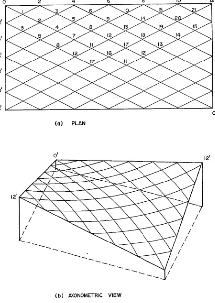
Fig. (5-1)- Views of a 240 ftx 120 ft Hyperbolic Paraboloid Cable Hoof.
—24-Chapter 5- Numerical Studies.
5.1 Neglecting Horizontal Displacements.
A hyperbolic paraboloid roof 240 ft, x 120 ft
rising by 12 ft from two opposite corners to the two adjacent
corners shown in fig.(5-1), was analyzed by using the method
mentioned in chapter 2, neglecting frame deformation. The
ordinates of the joints were first determined by solving
equations (2-5) for the roof. Equations (3-16) were, then for
mulated for the loaded roof and were solved to obtain the
resultant displacements. The calculations were done for one
quarter of the net consisting of 21 joints for equal loads at
all joints and a tension of 50 Kips in all the cables. With
the deformation of the frame neglected the number of equations
that had to be solved was twenty one.
The same roof was. analyzed using equations
(3-16) taking the deformation of the frame into account.;For
this purpose, the frame was assumed to consist of four beams
simply supported at their ends. The flexural rigidity of the 2
beams were taken as 96,000 Kip-in , The number of equations
in this case was thirty three; twenty one for the joints and
six for cables in each direction, the others being determined
by symmetry. In both cases the equations were, solved on the
IBM 8/360 computer using the available subroutine. The results
of the calculations are shown in tables (5-1) and (5-2).
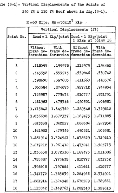
-25-Table (5-1)- Vertical Displacements of the Joints of
240 ft X 120 ft Roof shown in fig.(5-1).
E =50 Kips, BA=30x10^
Kip-Vertical Displacements (ft)
Joint No, Load = 1 Kip/joint Load = 1 Kip/joint 5 Kips at joint 16
Without frame de formation With frame de formation Without frame de... formation With frame de formation
1 .218095 .199978 .215975 .194460
2 .543592 .535913 .559846 .550742
5 .398608 .397683 .411660 .410576
4 .860394 .874873 .927712 .944904
5 .755987 .773634 .810777 .831731
6 .461982 .475346 .490521 .506381
7 1.115842 1.149762 1.289348 1.329612
8 1.036608 1.072337 1.169473 1.211885
9 .813359 .842227 .888684 . 922938
10 .461982 .475346 .490521 .506381
11 1.281914 1.324941 1.678529 1.729610
12 1.217212 1.261412 1.473241 1.525713
13 1.036608 1.072338 1.169473 1.211886
14 .755987 .773635 .810777 .831732
15 .398608 .397684 .411661 .410577
16 1.341772 1.383839 2.284966 2.334901
17 1.281914 1.324942 1.578529 1.729661
18 1.115842 1.149763 1.289348 1.329613
24869T
“ 2 6
-Table (5-1) (contd.)
Vertical Displacements (ft)
Joint No. Load = 1 Kip/joint Load» 1 Kip/joint 5 Kips at joint 16
Without frame de formation With frame de formation Without frame de formation With frame de formation
19 .860394 ,874874
.
927712 .944906 20 .543592 .535914 .559846 .55074421 .218095 .199977 .215975 .194460
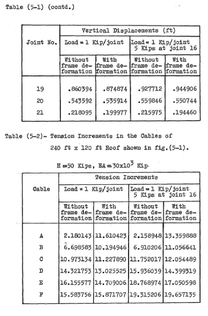
Table (5-2)- Tension Increments in the Cables of
240 ft X 120 ft Roof shown in fig.(5-1).
H = 5 0 Kips, EA =.30x10^
Kip-Tension Increments
Cable Load = 1 Kip/joint Loadssl Kip/joint 5 Kips at joint 16
Without frame: de formation With frame de formation Without frame de formation With frame de formation
A 2.180143 11.610423 2.158948 13.359888
B 6.698583 10.194946 6.910206 11.056641
C 10.973134 11.227890 11.752017 12.054489 D 14.321753 13.025525 15.936039 14.399319 E 16.155577 14.709006 18.768974 17.050598
F 15.583756 15.871707 19.315206 19.657135
o' 2' 10 12
20
I
2‘
26
32
I
4 ‘
.30. 24
2&
23
I
S'
33 2 8
32 27
8'
35.
34.
lO'
12'
Pig, (5-2-)- Plan of the 240. ft x 120 ft Hyperbolic Paraboloid Cable Roof.
-27-_
2 8
-5.2 Taking Horizontal Displacements into Account.
The roof referred to in (5.1) was analyzed
using the general theory given in chapter 4. In this case,
half the net was usedi for calculations since there is no
symmetry within half the net. There is only antisymmetry
about the diagonals. For example, for a joint like joint 5,
fig. (5-2) there, is a corresponding joint in the opposite
corner in the other half of the net which has the same vert
ical displacement but equal and opposite horizontal displace
ments as joint 3. Equations (4-9) were, written for the joints.
A program was written for the IBM S/360 computer to form the
108 X 108 matrix, solve the equations using the available
subroutine to obtain the displacements, modify the co-ordi
nates and recalculate the displacements until a satisfactory
convergence was reached. The tension increment in each section
of the cable was then calculated using the final displacements.
The program was also modified for the incremental load method
for comparison of the results. Plow charts for the two pro
grams and the computer program for the incremental load method
are shown in the appendix.
The calculations were performed for various
loadings and varying
parameters:-(i) Equal loads at all joints with H, the hori
zontal component of tension fixed at 50 Eips in all the
cables. The loads were increased by equal increments and the
nonlinear variation of the deflections obtained. Typical
results .are shown in table (5-3) and the behaviour of joints
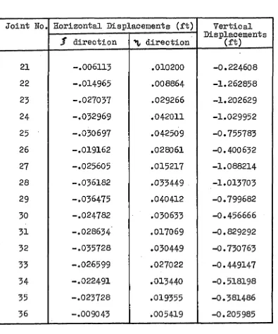
-29-Table (5-3)- Vertical and Horizontal Displacements of the
Joints of 240 ft x 120 ft Roof shown in fig,(5-2)
H =50 Kips, E A = 30x10^ Kip- Load= 1 Kip/joint
Joint No. Horizontal Displacements (ft) Vertical Displacements
(ft) f direction direction
1 .009043 -.005419 -0.205983
2 .022490 -.013440 -0.518198
3 .014274 -.003338 -0.382553
4 .028636 -.017070 -0.829292
5 .018983 -.002147 -0.732224
6 .005984 .007660 -0.450873
7 .025604 -.015218 -1.088215
8 .014322 .003442 -1.014998
9 .001917 .017658 -0.801635
10 -.004715 .018791 -0.458200
11 .014965 -.008864 -1.262860
12. .002812 .011588 -1.203370
13 -.008426 .027513 -1.031159
14 -.014310 .032873 -0.756990
15 -.011860 .023797 -0.401313
16 .000000 .000000 -1.328606
17 -.011429 .019288 -1.273480
18 -.019673 .033057 -1.115296.
19 -.021873 .036605 -0.866189
20- -.016670 .027870 -0.551684
-30-Table (5-3) (contd.)
Joint No. Horizontal Displacements (ft) Vertical Displacements
(ft)
S
direction ^ direction21 -.005113 .010200 -0.224608
22 -.014965 .008864 -1.262858
23 -.027037 .029266 -1.202629
24 -.032969 .042011 -1.029952
25 -.030697 .042509 -0.755783
26 -.019162 .028061 -0.400632
27 -.025605 .015217 -1.088214
28 -.036182 .033449 -1.013703
29 -.036475 .040412 -0.799682
30 -.024782 .030633 -0.456666
31 -.028634 .017069 -0.829292
32 -.035728 .030449 -0.730763
33 -.026599 .027022 -0.449147
34 -.022491 .013440 -0.518198
35 -.023728 .019355 -0.381486
36 -.009043 .005419 -0.205985
1 and 16 are. shown in figs. (5-3) and (5-4) respectively,
(ii) Equal loads at all joints and in addition a
concentrated load at one of the joints under the same condi
tions as in (i). The concentrated load was placed at various
joints and the calculations were repeated. The behaviour of
-31-the different joints are shown in figs. (5-5) to (5-8).
(iii) The pretension in the cables was r:varied -and",
the calculations performed for a symmetrical loading of
1 Kip/joint and an unsymmetrical loading of 1 Kip/joint in
addition to a concentrated load of 5 Kips at joint 2. The
behaviour of joints 1 and 16 with the change in pretension
is shown in figs.(5-9) and (5-10).
(iv) The ratio of the sides of the rectangle was
varied keeping the smaller side equal to 120 ft and H equal
to 50 Kips. This varies the obliquity of the angle between
the two sets of cables. The variation was from r, the ratio
of the sides of the rectangle = 1 which is an orthogonal net
with sin 0 = 0 , to r = 2 for a net with sin © = 3/5. Here too
the calculations were done for the two loadings mentioned in
(iii). The:behaviour of joints 1 and 16 with the variation
in the degree of nonorthogonality is shown in figs. (5-11)
and (5-12).
In all these cases, the approximate method of
correction for nonlinearity was used. In case (i) and case (ii),
the calculations were repeated with the incremental load
method for comparison.
•9
•8
•7
•6
5
•4
•3
•2
LINEAR THEORY
APPROXIMATE METHOD
INCREMENTAL LOAD METHOD
LOAD ( KIPS )
Pig.(5-3)- Deflection at Joint 1 of the 240 ft x 120 ft
Gable Roof under a Uniform load,(H-50 Kips,EA=30xl05 Kip) -32- '
h-ll.
o Ui Ü. iU o
0 1 LsJ >
6
5
4
3
2
LINEAR THEORY
-o APPROXIMATE METHOD
^ INCREMENTAL LOAD METHOD
6
4
0 2 3
LOAD ( KIPS )
Pig.(5-4)- Deflection at Joint 16 of the 240 ft x 120 ft
Gable roof under a Uniform load.
(H»50 Kips, EA=30x103 Kips)
lO o o lO «o 0) 00 H?
<û CM h-z o
~3
in Q<
< O a s û: h-I I ro CM a fn O ♦H 0 Ctf fH 0 0 (M . O (M O
CÛ -P 0 (D •H iH O
Ü -P cd
cS
o o
CM J H Td m -p •P d «H U -p o 0 m CM o 0 (D o o -P as «M
o Td 0 CM cd
'—-C»1 P> o 0 0 H »r4 •H M
o O O h) " - ) d \ 11 -P A<D •H M W “
0 K)
O H A
•H •H
-P kd Ü O
(D O
H >0 'A Ch cd II 0) O ÎÜ P P ' - '
1
M l
M l
-•H
( ± d ) N O I1 3 3 1 j3 0 1V3IJ.W3A
lO
lO o
10 in
U i
a.
k:
0)
Q
<
O
o
1x1
H < a: h-z w u
8
( i d ) NOI1331d3Q 1V3I1W3A
to in o o CO Q. (O Q LÜ a: j-z UJ u z o o E h O •H c D CÔ R 0 ■r) 0 . ovo O H « •P 0 r4 *H o cd h) Ü •p ■p ■d O d o H 0 ■P -P d p O -P -d- P CM 0 Ü 0 P o •P Ü <H d •
o m
>d Pi
VO P -H H d
m •P -P O
a
P H•H •H M O 0 O
•1-3 \ II •P P<!
oj iH w fcij
-to 0 H Pi
•H •H •P tp w
Ü O 0 o H "d 'A Vid 11 0 o td P Pt'-'
I d-■>A
faO
•rH
( Id ) N O I l O d l d d a 1V3I1W3A
o
o g oo olO
g Y:
z o
I
Q UJ
I
O z
8
( I d ) N0IJL331d30 1V3I1W3A
• 4 5
•40
•35
O "30
_j -25
•20
•15
LOAD “
LOAD = ï KIP/JOINT + 5 KIPS AT JOINT 2
•10
70 60
50
30 4 0
20
10
H ( KIRS}
Bïg'(5-9)- Variation of the Deflection at Joint 1 of the
240 ft X 120 ft Gable Roof with H. (EA=50xlo3 Kips)
LOAD = I KIP/JOINT
LOAD = I KIP/JOINT-h
5KIPS AT JOINT
210 20 30 4 0 50 60 '70
■ : : ;
. H ( KIPS)
ï'ig» (5-10a)“ Variation of the ïension Increment in--the Section
of the Cable between Joints 16 and 17 of the
240 ft X 120 ft Cable Roof .with H.(EA=30xl03Kips)
1-95 1-85 1-75 •65 I-li. 155 I t LU _J u. UJ Q 1-45 _i < o UJ > •35 125 M5
■o LOAD = I KIP/JOINT
LOAD = I KIP/JOINT + 5 KIPS AT JOINT 2
105
70 6 0
50 4 0
H ( KIPS ) 3 0
20
Fig.(5-10)- Variation of the Deflection at Joint 16 of the
240 ft X 120 ft Cable Hoof with H. (Ei^30xlo5 Kips)
OJ
ô lO o
lO o
lO CVI lO
to
( Id ) N0l±D31d3a 1V3I1W3A
Pig.(5-11)- Variation of the Deflection at Joint 1 of the
Cable Roof with R. (H=50 Kips,EA=30xlo5 Kips)
—40—
CH
If)
s o
o 8
lO
cvi 8
a:
( I J ) N 0 llD 3 n d 3 a 1V3I1W3A
l'ig* (5-12v)- Variation of the Deflection at Joint 16 of
the Cable Roof with R. (H=50 Kips ,EA*30xlo3E3.ps)
4 2
-Ohapter 6- Experimental Study
6,1 Description of Model.
In order to verify the theory and calculations,
an experiment was; performed on a small scale model, The model
was 6 ft X 3 ft with a difference in height of 9 ins. between
adjacent corners. The net consisted of five 1/8 in, diameter
aluminum wires in each direction. The bounding frame was of
four 12 in. deep channels welded to form a rectangular box.
Holes were drilled on the channels diagonally and along
straight lines to form the boundary of the model roof. The
wires were provided with screws at the ends for tensioning.
The wires were, glued together at the joints and hangers were,
suspended from the joints for loading the net.
The two sets of wires approximately took the
shape of parabolas, with the tv/o sets having opposite curva
ture, The total number of interior joints were thirteen and
heavy channels, used for the frame justified the assumption of
no frame deformation. The tensions in the wires were measured
by attaching strain gauges on the wire at the ends. The def
lections were, measured by dial indicators,
A plan of the net is shown in fig.(6-1),
Photographs 1 to 4 illustrate the model.
-43-Photograph 1- Top. View of the Unloaded Model
Photograph 2. A View of the loaded Model and the Datran Strain Indicating Equipment,
“44“
m
Ml
Photograph 3- Top View of the loaded Model
Photograph 4- Side View of the loaded Model.
-45-6,2 Experimental Procedure,
The wires were tensioned and the strains in
the wires were checked until the necessary tensions in the
wires were reached. The tensions in the wires were so adjusted
that their horizontal components were all equal to 50 lbs.
The dial indicators were then fixed and adjusted to zero and
the joints were loaded. The dial indicator readings were
noted. The loads were increased by equal increments of 1 lb
at a time to a maximum of 5 lbs. The readings were then re
peated while unloading.
Readings were also taken for concentrated loads
at various joints increasing from 1 lb to 6 lbs in addition
to equal loads of 1 lb at all the joints.
The experimental results and the theoretically
calculated results for the model are shown in figs,(6-2) to
(6—10),
Pig.(6-1)- Plan of Model.
—46—
•06
•05
(rt
04
i
Ü
ut
_i IL
03
<
y
Ê-02
>
•01
/
/ 1V.
/ IL.
/ ^k
L
THEORY
^ EXPERIMENT
0 2 3 4 5 6
. LOAD ( lbs)
I^g,(6-2)- Deflection at Joint 7 of the Model under a Uniform
Load,
• 0 7
•06
•05
^ 0 4
Z Q
u
Ul .J IL 03 ui
o
ai
om OP. >
•01
THEORY
EXPERIMENT
6
5
3 4
2 0
LOAD (lb s )
Fig,(6-3)- Deflection at Joint 9 of the Model under a Uniform
Load,
—48—
•07
•06
_ 05
v>
z
z o
h-O
UJ
_l Ü.
UJ Q
•04
■I L
d 0 3
H-OU
■02
•01
THEORY
EXPERIMENT
6
5 4
2. 3
0
LOAD (lbs)
Fig.(6-4)- Deflectioa at Joint 12 of the Model under a
Uniform load.
—50—
• 2 2 5
•200
•175
•150
•125
•100
•075
•050
•025
THEORY
EXPERIMENT
LOAD ( lbs)
Fig, (6.-5)- Deflection at Joint 2 of the Model under a Concentrated load at Joint 2,
CO z
i—
o Ui u.
'JÜ
Q
_J
<
0
1
-1
-51-•225
•200
•J75
•150
•125
•100
•075
•050
•025
THEORY
EXPERIMENT
6
0 2 o 4 5
LOAD ( lbs)
Fig.(6-6)- Deflection at Joint 7 of the Model under a Concentrated Load at Joint
•200
•175
•150
en
z
-125
Z
O
H -U LU
Li. LU Q •100
â y
LU
>
•075
•050
•025
THEORY
EXPERIMENT
6
5
0 2 3 4
LOAD (lb s )
Fig.(6-7)- Deflection at Joint 8 of the Model, under a
Concentrated Load at Joint 8.
•125
•100
to
z
•075
z
o
H o
lu
_1
•050
y cc UI
>
•025
T H E O R Y
EXPERIMENT
6
5 4
3
2 0
LOAD (lbs)
P i g . (6-8)- D e f l e c t i o n at J o i n t 9 o f the M o d e l u n d e r a
C o n c e n t r a t e d l o a d at J o i n t 9.
-54-•225
•200
•175
•150
O 125
-I -100
•075
•050
•0 2 5
THEORY
EXPERIMENT
6
4 5
3
0 2
LOAD (lb s )
Pig.(6-9)- Deflection at Joint 10 of the Model under a Concentrated load at Joint 1 0 .
-55-•225
•200
•175
•150
•125
z o
s
_J li.
LU
O
•100
<t o
h-•075
•050
•025
THEORY
EXPERIMENT
LOAD ( l b s )
Fig.(6-10)- Deflection at Joint 11 of the Model under a
Concentrated Load at Joint 11.
-56-Chapter 7- Discussion of Results.
1. The vertical displacements were calculated using the
approximate, method neglectirg horizontal displacements with
the deformation of the frame neglected in one case and with
the deformation of the frame taken into account in another.
The difference between the calculated values in the two cases
will; of course, depend on the stiffness of the frame. In the
case considered here, with E = 30x10^ Kips/in^ and I = 3200 in^
there is a maximum difference of between the two displace
ments but for most of the. joints, the difference is about 4^.
Whether or not it is necessary to consider the deformation of
the frame depends on the stiffness of the frame actually used,
2, The vertical displacements when calculated using the
general theory taking horizontal displacements into account,
differ from the values calculated by the approximate theory
by a maximum of 6fo, In addition to this difference, the hori
zontal displacements which were neglected in the latter theory
are significant, approaching 5 to 7^ of the vertical displace
ments when the former theory is used. These two differences:
combine together to give a larger error in the calculated
tension increments. Such increments in the two cases differ
by up to 12^ in the longer cables where the change in tension
is large. It is therefore necessary that the general theory
be used in the analysis of this type of roof in order to
-57-obtain accurate results, even though this involves three
times the number of equations.
3. It is also evident from the graphs jfigs. (5-5) to (5-8)]
that the load deflection behaviour is nonlinear for loads
larger than 1 Kip/joint for the roof considered here. In
creasing load has a ‘strengthening* effect on the net,i.e.
the corrected value is lower than the value obtained by the
linear theory. For smaller loads, it would be sufficient to
use the linear theory but for larger loads, this would result
in a conservative value for displacements and the tension
increments.
4. It is seen from the calculations that the value obtained
by the approximate method of correction for nonlinearity
almost coincides with the value obtained by the more accurate
incremental load method. The difference between the two values
is greatest when the loading is unsymmetricâl ^ i g . (5-5)] but
is negligibly small in the case of symmetrical loading [fig.
(5-6)]. It is sometimes timesaving to use the former, since
in most cases one is interested in the displacements under
a particular loading in which case solution, by the former
will require a few iterations whereas the latter might require
several increments to reach the particular value of loading.
The values obtained by the two methods deviate more as the
load increases but the amount of computing time taken with
the incremental load method over and above the approximate
method, also increases with the load and offsets the advantage
of the slightly more accurate results. For example, for equal
-58-loads of 4 Kips/joint, the first method requires 15 iterations
to converge within 1x10“^, while the incremental load method
requires 40 increments of 0.1 Kips each and the difference
between the two values is only about 3^ for a saving of 60^
of the computing time.
5. From a comparison of the deflection of joint 2 due to a
concentrated load at joint 2 and the deflection of joint 20
due to a concentrated load at joint 20, it is seen that the
nonlinearity is more marked when the loading is unsymmetricâl.
The former is unsymmetricâl while the latter is symmetrical
since it assumes a concentrated load in the opposite corner,
6.. The deflections and tension increments decrease with the
increase of H, the horizontal component of tension, as ex
pected. The deflections could be reduced by increasing the
pretension in the cables but this increased tension will have
to be accounted for at the edge beams and the anchorages. A
compromise, therefore, has to be struck and other factors
such as susceptibility to flutter also must be considered.
7. The deflection decreases as the degree of nonorthogona
lity of the net decreases and is a minimum when the net is
orthogonal. The horizontal displacements are also much smaller
in the orthogonal net than in a nonorthogonal net.
8. The experimental values agree with the theoretically
calculated values within reasonable limits. The difference
between the theoretical and the experimental values differ
by very small to large percentages but the average difference
can be said to be about 10-15^. The theoretical values are on
-59-the conservative side for most cases of loading and for most
of the joints. This is seen from figs.(6-2), (6-3) and (6-4)
for symmetrical loading and.from figures (6-6), (6-7) and
(6-8) for concentrated loads at joints 7,8 and 9 respectively.
The theoretical values are lower than the experimental values
only in the case of concentrated loads at joints 2,10 and 11
\figs.(6-5), (6-9) and (6-10)]. Since these latter joints are
less critical than the former joints from the design point of
view and since the theoretical values are on the conservative
side for most cases of loading, it may be said that in general
the theoretical values are on the conservative side.
9. The sources of error in the experiment may be one or
more of the
following;-(a) Inaccuracy in measuring the initial tension in the
wires and the value of EA used.
(b) Irregularity in the geometry of the model.
(c) Stiffness of the joints and the bending stiffness
of the wires which were neglected in the theory.
(d) Any deformation of the frame.
(e) Inaccuracy in' measuring the deflections.
(f) Inaccuracy of the theory.
Source (a) is likely because there would have
been an error in the measurement of the strain with the strain
gauges. A non-axial strain gauge alignment can introduce sig
nificant error. The value of E used was the value supplied
by the manufacturer for 6061 T6-El9 aluminum which was used.
6 0
-Source (b) is also likely due to irregularities in fabricating
the model and due to the finite thickness of the wire and the
joints.
The stiffness of the glued joints and the
bending stiffness of the wires would also introduce some error.
The measured deflection would have been somewhat inaccurate
due to friction in the dial indicators but this was eliminated
to some extent by using the average value of the readings
taken while loading and unloading. The deformation of the
frame could not have introduced any significant error, consi
dering its excessive rigidity. The theory too cannot be called
inexact since it is derived from first principles considering
the equilibrium of the system. Correction for nonlinearity
was applied by incremental load method and noting the very
small nonlinearity of the system, the error involved would be
negligible,
10. Since the nonlinearity of the model was smaller than the
accuracy with which the experimental results were obtained,
the nonlinear behaviour of the model could not be verified.
—61—
Chapter 8- Conclusions.
For the study presented herein, the following
conclusions can be
drawn:-1. For nonorthogonal nets the horizontal displacements
cannot be neglected in comparison to the vertical displacements,
Therefore the general theory considering displacements in all
directions has to be used. In the case of orthogonal nets,
however, the horizontal displacements are small and may be
neglected.
2. In calculating the vertical displacements of the joints,
the effect of deformation of the bounding frame may have to
be taken into account depending on the flexural rigfdity of
the edge beam used. This may become necessary in the case of
very long spans where the edge beam is used without intermedi
ate supports.
3. The load-deflection behaviour is nonlinear for large
loads. In applying correction for nonlinearity, the value
obtained by using the approximate method is not very much
different from that obtained by the incremental load method.
The former may be used in favour of the latter on account of
the appreciable saving in computing time for any one particu
lar set of loading. Furthermore, the nonlinearity is more
marked in 4;he case of unsymmetrical loading.
4. The deflections and tension increments decrease with the
—62-increase in pretension. They also decrease with the nonortho
gonality of the cables.
5. The experimental values are in fair agreement with the
theoretical values. The theoretical values are in general on
the conservative side. Nonlinear behaviour could not be verified-
experimentally due to the very small nonlinearity of the model
used. For future work, it is recommended that a more flexible
model be used so that the nonlinear behaviour of the system
could be more readily verified.
Appendix A- Plow Charts for Computer Programs.
^ Start ^
Read jrdinatesy
and maiirix
Read
iE,EA,R8,
Read load
Transfer initial or dinates to work area
Calculate
P(I)
Calculate
cos r ,sinîT
/ Perm \ / resultants
\ matrix. /
Rextl
—63“
dîlll pOBLVe
Modify coordinates
yes
Calculate tension
Incréments
Print displ. I ten- \sions
last load^^S-/ b
yes
//Last
larameter lo
yes
Plow Chart 1- Calculation of Displacements-Correction for
Nonlinearity by Approximate Method.
—64“
^ start ^
(Read ordi nates &
matrix) kcoeff,
Read
Transfer initial or dinates to work area
Initialize
displace
ments
Calculate
F(I)
onta.
F o r m
^result ant
m a t r i x
S o l v e for
ydisplace-m e n t s
n t e r m e d i a t e
l o a d ?
C a l c u l a t e
t e n s i o n
i n c r e m e n t s
A c c u m u l a t e M o d i f y
d i s p l a c e c o o r d i n a t e s
m e n t s
P r i n t
d i s p l . &
\tensioi Lncrmts
l o a d i n c ™ w o
m e n t ?
- 66—
on
■reatest V
load?-es
yes
,Mo
yes
STOP
Plow Chart 2- Calculation of Displacements- Incremental
Load Method.
- A P P E N D I X LISTING^ .02- A
SAMPLE._PRO.GRAM,-/ SAMPLE._PRO.GRAM,-/ C O W L O A O 1 1 1 ; 'ic G L _ i:V L L L = 1
r'--'0'i*s F-o • ^•-~—-—•■
--/ --/ F O R T . S Y S I N u J
i:-C T . K U , 4 - N : ' N ... ...;.ii_,l5-T-<iL— L iË —l- 1 V I I---u J ü I f - J ; - - K .
C i'^OIM — O R T L . Mi-'I—c.
..I__ . . -.G t£ N E .R A l A N « U .'tS .I.G - i-...,U > J G K L -,y c .jiiJ A i„ L U A J - . . . J J £ X b R U .
C C O N C c N T W A T u U L Oa u
1 • R G A D InP Ui U /'-iT A
-C-O I M E N S I O N m X 1 ( 0 6 , 3 6 ) , A X 3 ( 3 6 , 3 6 ) , A X j ( 3 6 , 3 6 ) , A X 4 ( 3 o , 3 6 ) , A X33 C 3 o , 3 6 )
. 3 - U à E N S . L ü N . - .a6±.(_l..A.8._,.3..v-8-).-,..6.M3_U..36-,..1.3.3J,,j, A:.iX_Li.3a3_lA-â-)_________________________
0 I M E N S I O N 6 ( 1 3 6 ) , Ü 1 ( K ; 8 ) , 2 ( 3 6 ) , Z 1 ( 3 6 ) , F ( 6 ) , 3 U ," i ( 3 ) , R ( 6 ) , 3 l 3 ( 1 Oc _______ 0 -IM E - N S - I 0 N .-C '3 S G - C .3 6 .» -4 .) -,- S I.,N G ,(.3.q.,..4..)--- ,.ü Z L Z ..( ..3 .6 ..;Æ ) ---
;---R E A ü l l ü , ( 2 1 ( 1 ) , 1 = 1 , 3 6 )
-44-g-A2)R34AX_(-6H .1.2u.AU-
---R E A D 1 2 3 , ( (aX 1 ( I , J ) , J = 1 , 3 6 ) , I = 1 , 3 6 )
— ,. _l-^_ -\.J-..,-.(—( . / I .(.1..,-.^^.J—,—xJ—™...X—,..xX_^J,.).—1—.—1.,,,.._xX_XX.)„... --- — — , .— ,— — .— -... ...— —.
R E A D 1 2 0 , ( ( mX 3 { 1 , J ) , J = 1 , 3 6 ) . , 1 = 1 , 3 o )
... — 'iOiA*A‘i3— 1 — , —(--(—^■-X'^T” ( —1'",—O"')—,'x.)"” ' 1—,“<3xx-)—, —I—™-1— . )—
---1 2 u F O R M A T ( I d F J . U )
--- iR trA G l— l-3"6-,~C-R-(—I—)—,—l- = - l—,- 6 - )
---—---1 3 0 F O R M A T ( 6 F 1 0 . Ü )
—2 I... ' “ ( -t' —^ . 1— — 1 —I— . XX-. 1—.. X. — 1—) . . . — . . —.. —II.. ... I — - .. — — —..—..———.—.— ——..II..——.—I.
P R I N T 1 5 u
-l.-aQ.i.-F-ORiMAA'— (.-l.-I-Hw-I-NRU-T— UA-T-Â-)--- — --
---1 5 5 F O R M A T ( 4 H 3 H = , F 6 • 1 , 5 X , 4 H E A = , F d • 1 , 5 X , 1 2 M S I iN ( T H E T A ) = , F 1 0 . d )
1 6 “ F O R M A T L6H -3L.U 3\u.._.N O ,,__L4L2_(..l.kla..,.i . 8 F 6 .<l1 D J ---1 7 0 F O R M A T ( 1 3 H 0 0 R D I NaT E S / ( 1 H o , V F 1 2 . 8 ) )
-.1-d.u— F O R M A-T U _ x 4 d ju u a X _ ù l aX R - IX Z - C - Ll-Lo.jL .l_ d F -6 -*-l..i).-)-1 8 5 f o r m a t ( 5 Hx, R , 6 F l u . d )
e a.iN%— i._9_J_________ I___ :
-P R I N T 1 7 3 , ( 2 1 ( ! ) , ! = 1 , 3 6 )
-|= lr_ L )4 T — 1-8 2 2 ,_(_k4.( .1 .).,. 1,1= i..« -6
J---190 FORMAT (dH^RASULTS)
C 2 . C A L C U L A T E F ( l )
2 0 5 R E A D 1 4 0 , H , L a , « S
---iELO—0 ---2 0 0 L D = 3
D O 1 3 5 1 = 1 , 3 0
- 1 93 ' 2 '( T ) = 3 :1 ( T ) - ... D O 2 3 0 1 = 1 , l o d
-23-':^-D-I-o-<-I-)-=-o-.ax
---) 5 R E A D 1 2 o , ( I.! 1 ( I ) , I = 1 , 1 0 6 )
— A '= “ T‘3 -*‘ Q-'2jL)R"T—(' 1—« 3 3 " R ^ Xi'_-/v'E—) — ---3 1 N T = ( R S * * 2 - 1 . 0) / ( R 3 * * 2 + l . 0 ) G O -S T -= -S Q R T ( - l - » - o - S - I N T 3 L * 2 - ) ---
-P R I N T 1 5 5 , H , L A , 3 I N T
D O — 2 -2-0— L = L U ,2 L _ --- —
---3 0 ;’l ( I ) — ---3 • ---3
2 1 3 S U M ( I ) = 3Ui'-'i ( 1 ) + R ( J )
501=1**2
__________2 -~ v _ -E L (-J —)-=_______ I I ^ -X- ( 1 « w + 6 * u / ' 3 # ^ * 3 0 M ( 1 ) 2 ( ( 2 * 0 ^ 1 ) )
P R I N T 2 3 3 , A , ( F ( 1 ) , 1 = 1 , 6 )
I- 2 9 .0 .1 FO R M 'i aT ... ( F I d a 8 .2 ( o . F . l. u . » o ) ) ... ^— ... —... ... ... ... 2 4 0 L D = L D + 1 0
![WoNeF, an improved, extended and evaluated automatic French translation of WordNet (WoNeF : amélioration, extension et évaluation d’une traduction française automatique de WordNet) [in French]](data:image/gif;base64,R0lGODlhAQABAIAAAP///wAAACH5BAEAAAAALAAAAAABAAEAAAICRAEAOw==)