INTERFACE PHENOMENA IN PROTON EXCHANGE MEMBRANE FUEL CELLS

(1)

University of Windsor University of Windsor

Scholarship at UWindsor

Electronic Theses and Dissertations Theses, Dissertations, and Major Papers

2011

INTERFACE PHENOMENA IN PROTON EXCHANGE MEMBRANE

FUEL CELLS

Simo Kang

University of Windsor

Follow this and additional works at: https://scholar.uwindsor.ca/etd

Recommended Citation Recommended Citation

Kang, Simo, "INTERFACE PHENOMENA IN PROTON EXCHANGE MEMBRANE FUEL CELLS" (2011). Electronic Theses and Dissertations. 5389.

https://scholar.uwindsor.ca/etd/5389

This online database contains the full-text of PhD dissertations and Masters’ theses of University of Windsor students from 1954 forward. These documents are made available for personal study and research purposes only, in accordance with the Canadian Copyright Act and the Creative Commons license—CC BY-NC-ND (Attribution, Non-Commercial, No Derivative Works). Under this license, works must always be attributed to the copyright holder (original author), cannot be used for any commercial purposes, and may not be altered. Any other use would require the permission of the copyright holder. Students may inquire about withdrawing their dissertation and/or thesis from this database. For additional inquiries, please contact the repository administrator via email

(2)

INTERFACE PHENOMENA IN PROTON EXCHANGE MEMBRANE

FUEL CELLS

by

Simo Kang

A Thesis

Submitted to the Faculty of Graduate Studies

Through

Mechanical Engineering

in Partial Fulfillment of the Requirements for

the Degree of Master of Applied Science at the

University of Windsor

Windsor, Ontario, Canada

2011

(3)

Interface phenomena in proton exchange membrane fuel cells

By

Simo Kang

APPROVED BY:

Dr. Xiaobu Yuan, Outside Reader

School of Computer Science

Dr. Andrzej Sobiesiak, Program Reader

Department of Mechanical, Automotive & Materials Engineering

Dr. Biao Zhou, Advisor

Department of Mechanical, Automotive & Materials Engineering

Dr.

Jennifer Johrendt, Chair of Defense

(4)

iii

Declaration of Co-Authorship / Previous Publication

I. Co-Authorship Declaration

I hereby declare that this thesis incorporates material that

is result of joint research,

as follows:

This thesis also incorporates the outcome of a joint research undertaken in

collaboration with Chin-Hsiang Cheng, Huan-Ruei Shiu and Chun-I Lee and under

the supervision of professor Biao Zhou. The collaboration is covered in Chapter 4 of

the thesis. In all cases, the key ideas, primary contributions, experimental designs,

data analysis and interpretation, were performed by the author, and the contribution of

co-authors was primarily through the provision of financial support and participate in

the discussion of modeling results.

I am aware of the University of Windsor Senate Policy on Authorship and I certify

that I have properly acknowledged the contribution of other researchers to my thesis,

and have obtained written permission from each of the co-author(s) to include the

above material(s) in my thesis.

I certify that, with the above qualification, this thesis, and the research to which it

refers, is the product of my own work.

II. Declaration of Previous Publication

This thesis includes one original paper that has been previously published for

publication in peer reviewed journals, as follows:

Thesis

Chapter

Publication title/full citation

Publication

status*

Chapter 4 Liquid water flooding in a proton exchange membrane

fuel cell cathode with an interdigitated design

，

S Kang, B

Zhou, C Cheng, H Shiu, C Lee, Liquid water flooding in a

proton exchange membrane fuel cell cathode with an

interdigitated design, Int. J. Energy Res. (2011),

DOI: 10.1002/er.1858

(5)

iv

I certify that I have obtained a written permission from the copyright owner(s) to

include the above published material(s) in my thesis. I certify that the above material

describes work completed during my registration as graduate student at the University

of Windsor.

I declare that, to the best of my knowledge, my thesis does not infringe upon

anyone’s copyright nor violate any proprietary rights and that any ideas, techniques,

quotations, or any other material from the work of other people included in my thesis,

published or otherwise, are fully acknowledged in accordance with the standard

referencing practices. Furthermore, to the extent that I have included copyrighted

material that surpasses the bounds of fair dealing within the meaning of the Canada

Copyright Act, I certify that I have obtained a written permission from the copyright

owner(s) to include such material(s) in my thesis.

(6)

v

Abstract

Two phase flow phenomena is a critical issue in Proton Exchange Membrane Fuel Cell (PEMFC) development. Two main classes of PEMFCs, direct hydrogen fuel cell (DHFC) and direct methanol fuel cell (DMFC) have similar problem caused by two phase flow. Both the water in cathode (DHFC and DMFC) and CO2 in anode (DMFC) cannot be removed

efficiently will hinder the process of the chemical reaction of the fuel cell and interfere with the performance. To optimize the performance of a PEMFC, it is important to understand the gas-liquid interaction and an accurate two-phase modeling needs be develop for this purpose.

(7)

vi

Dedication

(8)

vii

Acknowledgements

I would like to express my deepest gratitude to my supervisors, Dr. Biao Zhou, for the guidance provided throughout the course of my research, his constructive criticism, many valuable suggestions and continuous support.

My thanks also go to Dr. Xiaobu Yuan and Dr.

Andrzej Sobiesiak

for all their help and support to develop this thesis.

I specially thank all the members and previous members of the Dr. Zhou’s laboratory with whom I had numerous fruitful discussions, in particular Xichen Wang.

I specially thank those who provided kindly and effective help among faculty, staff, and students at the University of Windsor.

(9)

viii

List of Tables

Table 1-1 Comparison of DHFC and DMFC [1–3] ... 4

Table 5-1 Effect of liquid viscosity ... 51

Table 6-1 Parameters and properties used in the model ... 54

Table 7-1 Parameters and properties used in the model ... 68

(13)

xii

List of Figures

Fig. 1-1 PEMFC structure ... 3

Fig. 3-1 Computational domain ... 13

Fig. 4-1 Computational domain and definition of the components ... 17

Fig. 4-2 Comparison of numerical simulation and experimental visualization ... 18

Fig. 4-3 The general process of water behavior shown with 3D isosurfaces ... 20

Fig. 4-4 Water volume fraction and velocity vector in the selected cross section in the porous layer (Z = 0.15 mm) and the water volume fraction and velocity vector in the selected cross section in the flow channels (Z = 0.45 mm) ... 22

Fig. 4-5 Water volume fraction and velocity vectors in the cross sections (X = 12 mm and X = 15 mm) at t = 0.419 s ... 29

Fig. 4-6 Water volume fraction and velocity vectors in the cross sections (Y = 6 mm, Y = 12 mm, and Y = 18 mm) at (2) t = 0.006 s, (3) t = 0.015 s, (4) t = 0.091 s, (5) t = 0.156 s, ... 32

Fig. 4-7 Water outflow process from the outlet channel shown from the XY view at (1) t = 0.753 s, (2) t = 1.367 s, (3) t = 1.383 s ... 34

Fig. 4-8 Liquid water distribution in the 3D outlet channel and in the cross sections at (1) t = 0.753 s, (2) t = 1.367 s, (3) t = 1.383 s, (4) t = 1.388 s, (5) t = 1.391 s, (6) t = 1.393s ... 37

Fig. 4-9 The avalanche process and the draining process shown from the XY view at (1) t = 1.138 s, (2) t = 1.155 s, (3) t = 1.178 s, (4) t = 1.277 s ... 38

Fig. 4-10 Variation curve of the amount of water as a function of time in the entire domain ... 40

Fig. 5-1 Computational domain of serpentine channel ... 42

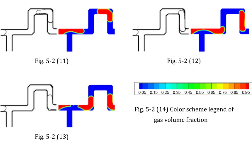
Fig. 5-2 Validation with bubble generated in T-junction ... 44

Fig. 5-3 Gas volume fraction and velocity vector in T-junction ... 46

Fig. 5-4 Volume fraction of Gas and Pressure distribution in serpentine channel ... 48

Fig. 5-5 Volume fraction of gas and pressure drop with vector of first two inverted U shape channels ... 49

Fig. 5-6 Gaseous volume fraction of two cases with different surface tension ... 50

Fig. 6-1 Computational geometry ... 53

Fig. 6-2 General process of gas CO2 flooding ... 55

Fig. 6-3 CO2 distribution at Z =-0.00015 m ... 57

Fig. 6-4 General process by which liquid water emerges into the channels ... 59

Fig. 6-5 CO2 volume amount in different part of the computational domain ... 60

Fig. 6-6 Pressure of each sub-domain inlet and outlet ... 65

(14)

xiii

innovation GDL ... 67

Fig. 7-2 Innovation gas diffusion layer (GDL) ... 68

Fig. 7-3 Comparison of numerical simulation and experimental visualization ... 69

Fig. 7-4 The general process of gas behavior shown with 3D isosurfaces (first column I) and selected cross-section (second column II), and the part of the corss-section has been enlarged to see the vector ... 74

Fig. 7-5 Comparison of emerging process of gas in two cases with same boundary condition but different gravity orientation: ... 76

Fig. 7-6 Gas volume fraction and velocity vector in the selected cross section in the porous layer ... 78

Fig. 7-7 Gas volume fraction and velocity vector in the selected cross section in the porous layer ... 80

Fig. 8-1 Gas diffusion layer built in this model ... 82

Fig. 8-2 Validation of simulation results with visualization study results of DMFC anode with a parallel design by Liao et al. [58] ... 84

Fig. 8-3 General process of gas CO2 flooding process with and without dynamic contact angle considered ... 86

Fig. 8-4 Comparison of emerging process of CO2 of two cases with static contact angle (left column) and with dynamic contact angle (right column) on cross-section of Z =–0.00005 m in GDL ... 88

Fig. 8-5 The contact angle of wall around the GDL and CL in the case with DCA ... 88

Fig. 8-6 Gas CO2 volume amount inside each sub-domain ... 90

(15)

xiv

Nomenclature



_{Density (kgm}

3

₎



_Porosity

u

Velocity vector (ms

-1

)

S

_{Source term}



Phase volume fraction



_{Dynamic viscosity (Pas)}



Surface tension (Nm

-1

)



Surface curvature

K

Permeability (m

2

)

n

_N

ormal vector

D



Dynamic contact angle (°)

e



Contact angle in equilibrium (°)

Ca

Capillary number

Hoff

f

Hoffmann function

1 Hoff

f

Reversed Hoffmann function

* Hoff

f

Improved Hoffmann function

x

Shift factor

Vel

Contact line velocity (ms

-1

)

Subscripts

1 Liquid phase

(16)

1

Chapter 1 Introduction

1.1 Fuel cells

1.1.1 General descriptions

A fuel cell is an energy conversion device that transforms the chemical energy stored in a fuel into electrical energy through an exothermic electrochemical reaction. Unlike a battery, a fuel cell does not deplete or require recharging. It generates electricity continuously as long as fuel and oxidant are supplied. A fuel cell usually contains two electrodes (an anode and a cathode) separated by an electrolyte. Two couple half reactions occurred at the electrodes: an oxidation reaction liberates electrons at the cathode side; a reduction reaction consumes electrons at the anode side [1, 2].

Compared with combustion engines, fuel cells are much more efficiently and environmentally friendly without NOx, SOx and particulate emissions. As a result, fuel cells

are considered as potential alternatives to the fossil fuels. Meanwhile, they offer higher potential power density compare with battery and fast response to charge of load. Furthermore, fuel cells present even more intriguing advantages, such as mechanical simplicity, modularity, lower noise level, quick start-up.

However, fuel cells are not perfect with some serious problems, for example, highly cost, low power density, storage and availability of the fuels, operational temperature. Fuel cells cannot be extensively applied without approaches to these problems [1].

1.1.2 Classification of fuel cells

(17)

2

temperature for each type of fuel cells is different, ranging from 30–100 ℃ for PEMFC, 160–220 ℃ for PAFC, 60–250 ℃ for AFC, 600–800 ℃ for MCFC, and 600–1000 ℃

for SOFC.

1.2 PEM fuel cells

1.2.1 PEMFCs Principle

The PEMFC is named because of the special proton-exchange membrane that it uses as its electrolyte. It can be sub-classified by the fuel it used. The most common fuel for the PEMFCs is hydrogen. Usually, the hydrogen needs to be produced from various fuels through a reforming process, such as methane, methanol, and gasoline. In recent years, using methanol as a fuel which could directly consumed in fuel cells without the deforming process also present intriguing advantages. This kind of fuel cells is named direct methanol fuel cell (DMFC).

Figure 1.1 shows the basic component of a PEM fuel cell. A proton conducting membrane is sandwiched between the anode and the cathode side. In each side, it include anode or cathode catalysts layer (CL), gas diffusion layers (GDLs), and channels in a bipolar plate. In a direct hydrogen PEM fuel cell, hydrogen which introduced through the channels cross the GDL and get the anode catalyst layer. With the presence of catalyst, the hydrogen dissociate into protons and electrons. The membrane is attached by both anode and cathode CLs. While the electrons generated in the anode CLs, they are unable to go through the membrane as the protons do. As a result, current generated [4].

As introduced above, the PEMFC could be sub-classified according to the fuel used. One of main type of PEMFC is hydrogen proton exchange membrane fuel cell. Usually it is called PEMFC directly because of the long developing history before other types of PEMFC. However, in this thesis, relative directly methanol fuel cell (DMFC), hydrogen PEMFC is called directly hydrogen fuel cell (DHFC) to distinguish.

The two major reactions occurring in a DHFC are hydrogen oxidation reaction at anode and oxygen reduction reaction at cathode as followed:

2

2 2

2 2 2

2 2

1

2 2

2

1/ 2

H H e

O H e H O

H O H O

 

 

  

(18)

3 Proton exchange membrane Anode plate Catalyst layer Gas diffusion layer Cathode plate

e- _e

-2 2

2 2

:1/ 2 2 2 :3/ 2 6 6 3

DHFC O H e H O

DMFC O H e H O

 

  

2

3 2 2

: 2 2

: 6 6

DHFC H H e

DMFC CH OH H O H e CO

 

 

   

Fig. 1‐1 PEMFC structure

The fuel in the DMFC is changed to methanol, and the cell reactions are changed to:

3 2 2

2 2

3 2 2 2

6 5 6

3

3 6 6

2

3

2 2

CH OH OH H O e CO

O H O e OH

CH OH O H O CO

 

   

  

  

Today, the catalyst used for both anode and cathode reaction is platinum. Adopting platinum could reduce the loss of cell voltage potential with methanol oxidize in cathode. However, this catalyst is not enough for the reduction of oxygen, which results low efficient on lessen of methanol crossover. During the methanol oxidation reaction, carbon dioxide (CO) is also formed and adsorbed onto the catalyst. This will affect the performance of the cell by reduce surface area. Meanwhile, other components in the catalyst layer, such as ruthenium or gold tends to improve this performance because these catalysts oxidize water to yield OH radicals:

2

H OOH He_.

Then the OH species could react with CO and generate CO2.

2

(19)

4

1.2.2 Advantages

First, lower operating temperature makes PEMFCs easier to operate. They are usually could rapid start-up and change the power output.

Second, solid electrolyte results less expensive to manufacture. Different with liquid electrolyte, solid part helps sealing the anode and cathode fluid (liquid and gas). Also, because of the solid electrolyte do not have the problems like orientation and corrosion, they make the PEMFCs a longer life.

Table 1‐1 Comparison of DHFC and DMFC [1–3]

DHFC DMFC Electrolyte Proton exchange membrane Proton exchange membrane

Fuels Hydrogen Methanol and water Operating Temperature (◦C) 30–100 30–100

Charge carrier H+ _H+

Catalyst Pt Pt/Ru

Operation pressure (atm) 1–3 1 (Anode) 1–3 (Cathode)

Advantages

Low-temperature operation；

High efficiency；

Relatively rapid start-up；

Zero-emissions；

High H2 power-to-weight ratio；

Hydrogen can be produced at either large or small facilities.

Low-temperature operation; High efficiency; Relatively rapid start-up;

Zero-emissions; High energy density of MeOH; Ease of produce and transport of

MeOH.

Disadvantages

Water management; Expensive catalyst; Durability of components not yet

sufficient; Poor-quality waste heat;

Intolerance to CO; Thermal management.

CO2 bubble management in anode;

Water management in cathode; Expensive catalyst; Durability of components not yet

sufficient; Poor-quality waste heat;

(20)

5

Third, the PEMFCs brought no air-pollution with zero-emission. Because of the only product are water and heat, the DHFCs are considered to produce drinking water.

DHFC is more matured with longer history and more research concern because of its higher power-to-weight ratio. Nevertheless, for the application of small and portable devices, DMFCs showed their merit. Compare with hydrogen, methanol is much more easy to produced and transport and could be utilized in the fuel cells without passing through an expensive reformer. Although the power-to-weight ratio of methanol is only 1/5 of hydrogen, methanol could offer 4 times power density per volume under 250 atm because it is liquid.

1.2.3 Challenges

DHFC

During the commercialize progress of DHFC, there are still some serious technical issues for the fuel cell researchers: (1) two-phase flow management in cathode side (2) management of heat, (3) durability, and (4) freeze-thaw cycling and frozen-start capability.

Water management is a critical challenge for high-performance DHFCs. In the cathode side of DHFCs, oxygen reacts with protons transferred via a membrane and with electrons through an external circuit from the anode to generate water and release heat in the catalyst layer. Of the designs available in the literature [5], liquid water flooding typically occurs if the operating condition deviates from its nominal condition. Deviations in the operating conditions are unavoidable for practical engineering applications of DHFCs, such as fuel cell powered vehicles. Therefore, to commercialize DHFCs, the liquid water flooding process must be understood and properly resolved.

DMFC

Although DMFC has been recognized as one of the most promising portable fuel cell which could be commercialized, there is also some technological problem during the development of DMFC: (1) two-phase flow management in the anode and cathode [6, 7], (2) methanol crossover [8, 9], (3) poor catalyst activity, (4) high catalyst loading, (5) management of heat [10], (6) relatively low power density [11], (7) management of water [12-13], (8) slow reaction kinetics of methanol electro-oxidation.

(21)

6

should be removed from the anode outlet as efficiently as possible. Otherwise the bubble of CO2 choked in the anode channel would increase the gradient of methanol concentration

along the channel and hinder the continuous reaction. As a result, gas management in the anode side is a critical challenge for high-performance DMFC.

1.3 Objectives

In conclusion of the introduction above, it is easy to realize the critical problem for both DHFC and DMFC—two-phase flow phenomena. The interface phenomenon of liquid-gas is the central topic of the thesis.

Various general PEMFC model (both for DHFC and DMFC) are developed to investigate the interface phenomenon in PEMFC anode and cathode with various flow field. The volume of fluid (VOF) algorithm is adopted to track the interface. The accelerated model is used to get the effect of both two phase interaction and accumulation of fluid. Different porous layers were adopted to explore the best method to simplified simulation GDL and CL.

Through these numerical studies, the objectives could be summarized as follows:

 Gas-liquid interface tracking through multi-phase, three-dimensional PEMFC model;

 Tracking the distribution of liquid water in DHFC cathode with an interdigitated design;

 Tracking the distribution of CO2in DMFC anode with a parallel design;

 Tracking the liquid water flooding phenomena forming process;  Validated VOF algorithm application in bubble flow field;

 Improve the simplified model application on PEMFCs model, especially in DMFC anode;

(22)

7

Chapter 2 Literature review

2.1 Review of PEMFC numerical simulation

2.1.1 Review of DHFC numerical simulation

At the end of the previous century, many researchers were involved in fundamental investigations into the basic operating principles of DHFCs, especially for the transport mechanism of hydrogen ions through membranes [14-18]. Since the beginning of the 21st century, high-performance computing techniques and advanced numerical algorithms have been employed in DHFC modeling [19-21]. However, in these studies, only single-phase flow (i.e., no liquid water was considered) was simulated. Although this simplification provides some insight into the physics of the DHFCs, it cannot be applied to real applications with DHFCs in which liquid water exists during most of the operations.

Numerous researchers such as You and Liu [22], Wang et al. [23], and Cha et al. [24] have developed two-phase flow models in which liquid water was considered to be water vapor to simplify the modeling process. These developments significantly improved the understanding of simulations with two-phase flow. Unfortunately, these so-called two-phase flow models are essentially multi-component single-phase flow models in which the liquid water that is treated as water vapor is only an additional species for the conventional single-phase model. Therefore, these models provide some important information about the water vapor, but the information regarding the water in the liquid phase is not included; thus, the interface between the gas phase and the liquid phase cannot be predicted.

(23)

8

The behavior of liquid water inside the flow channels of single cells and cathode stacks was investigated by Zhou et al. [30-32] by using a volume of fluid (VOF) method that can directly track the interface between the gas phase and the liquid phase. However, these studies only focused on liquid water in the flow channels without considering the GDL and catalyst layer. Zhou et al. [33] also developed a general model for DHFCs in which a two-phase flow VOF model was coupled with detailed thermo-electro-chemical submodels. This general model of DHFCs can provide detailed information of the fluid flow, heat transfer, water behavior, and movement of electrons and ions. This model is state-of-the-art for DHFC modeling; however, it requires a large amount of computational resources. In a recent study, Zhou et al. [34] used the VOF algorithm to explore water behavior in serpentine flow channels and obtained a similar water deformation process and spatial-temporal position between the experimental visualization and numerical simulation. However, this simulation set the water inlet in the form of droplet injected from a pinhole, which caused some inconsistency compared to the actual liquid water generated in the fuel cell. Another type of water inlet with an initial distribution of water film that was used in an earlier study [30] had a similar problem. Of these water inlet methods, the method that emits water from the back surface of the porous layer with an accelerated model [35] is the best method to improve the fidelity of the simulation.

Accelerated models actually have been commonly used in life tests and other areas [36-41], but the application of this method in fuel cells related research was conducted by Zhou et al. for the first time [35]. The Chapter 4 of this thesis employs this method to shorten the computational time without sacrificing the major physics of liquid water flooding process.

2.1.2 Review of DMFC numerical simulation

With the development of DMFC, a number of studies have verified the CO2 bubble have

(24)

9

chose lattice-Boltzmann and VOF methods to explore the CO2 bubble dynamics. As their

compare result, lattice-Boltzmann and VOF model are both effective ways to track the interface of two-phase flow but the application for complex geometry hasn’t been explored.

For the objective of this thesis, VOF model is introduced to solve the two-phase problem in anode side of the DMFC. With the interface reconstruction scheme, the interface could be calculated more accurately.

According to study in Chapter 4, employing a volume of fluid (VOF) method is advantageous to track the interface between the gas phase and the liquid phase. It is possible to give further attempts to use VOF methodology to solve the similar problem of two phase flow in DMFCs. Chapter 5–8 developed a few different model of simplified DMFC anode with VOF method. A new geometry of GDLs was investigated. Like introduced above, GDL usually made of carbon paper or carbon cloth, the size of the pores of conventional GDLs are arbitrary, and the sizes of the pores are very small. Zhou et al. [49] designed a GDL with different micro-flow channels to solve liquid water flooding problems in conventional GDLs of DHFC. This design simulated the small holes in GDL without effective for water removal in the fluid channel, but neglected the effect of fluid convection inside GDL. In this study, the pores in GDL are well designed with uniformly holes distributed in a 0.1mm thickness porous layer sandwiched by a 0.1 mm thickness catalyst layer (CL) and a parallel designed channel on the other side.

2.2 Review of PEMFC experiment visualization

2.2.1 Review of DHFC experiment visualization

(25)

10

2.2.2 Review of DMFC experiment visualization

Different with DHFC cathode, more researchers tend to study the gas remove problem in DMFC anode by experiment. Pan et al. [56] explored the nucleation and growth of CO2

bubbles generated by chemical reactions of sulfuric acid and sodium bicarbonate in three different types of micro-channels, and simulated this experiment. Xiong et al. [57] analysed the bubble generation and transport in a microfluidic device with high aspect ratio. Effect of liquid viscosity and surface tension were discussed accordingly. These studies have remarkable insight into gas bubble behaviors in the anode channel of DMFCs. However, two phase interaction cannot be predicted.

Meanwhile, many experiments of DMFC with visualization study of CO2 bubble behavior

in anode channels were set up, the effect of aqueous methanol solution flow rate, temperature, and concentration with serious of experiment were discussed [58, 59]. Experiment provide a good visualization data for CO2 bubble behaviors in the flow channels, however, detailed

(26)

11

Chapter 3 Numerical model setup

3.1 Governing equations

In the thesis, FLUENT [60] was used with a 3D unsteady VOF model to perform the numerical simulations and to track the gas–liquid interface inside of the computational domain. A UDF was applied in the calculation. The flow in the gas phase was assumed to be laminar. And pressure based solver was chosen with the first order implicit scheme.

The mass conservation law that governs unsteady, laminar flow can be written as:

( )

( u) 0 t



_

 _{  } _

 (1)

For multi-phase flow, the mixture density can be defined as:

2 2 (1 2) 1

      (2)

where subscript 1 mean the primary phase and 2 means the secondary phase (liquid water in DHFC, and gas in DMFC).

Volume fraction of the secondary phase 2_{could be solved by the volume fraction}

equation as followed:

2 2

( )

( u) Sf

t

 

_{ }

 _{  } _

 (3)

In this simplified model of PEMFC, S_f 0.

The details of the VOF equation will be presented in next section. The momentum equation can be expressed as:

u ( u)

( uu) p ( u)+ g+S

t



_

_

_

_

 _{  } _{    } _

 (4)

where    ₂ ₂ (1  ₂) ₁, p is the static pressure, εis the porosity, and u is the

velocity vector.

(27)

12

2

1 2

( ) / 2

u

S



 



 

 (5)

where σ is the surface tension coefficient, ρ represents the density, κ represents the surface curvature, which is defined in terms of the divergence of the unit normal ˆn:

ˆ n

n n



   

where n ₂ is the surface normal that is defined as the gradient of 2.

For the momentum equation in the porous layer, the source term is expressed using the second term on the right-hand side as an additional resistant force due to the porosity and permeability inside of the porous layer

2

1 2

u

( ) / 2

u S K

 







 

  

 (6)

where K represents the permeability.

3.2 Interface tracking algorithm

In this model, PLIC (piecewise linear interface calculation) VOF tracking methods is implemented because it is accurate and applicable for general unstructured meshes [61].

The basic concept of VOF model is computation of convection and diffusion fluxes through a computational domain with impact of source terms inside the domain. With this computation, the volume fraction of each cell would be figured out and the interface will be reconstructed in each cell through an interpolating formulation.

The VOF geometric reconstruction process need go through two steps: reconstruction and propagation. The mainly objective of reconstruction step is segment of the interface inside the cell.

As the unit normal vector n and the volume fraction value are computed in the VOF

(28)

13

3.2.1 Interface reconstruction algorithm

As presented above, the objective of PLIC methods is determine a straight line in each cell. During this process, a estimation of straight line which perpendicular to an interface normal vector ni,j and divide the two volume for phases. The normal vector ni,j is determined from the

neighboring cells based on block’s



_{i j}_, of 9 cells as shown in Fig. 3-1.

The normal vector ni,j could be calculated from



i j, , ni j,  



i j, . Initially, a cell corner

value of the normal vector ni,j is computed. An example at i+1/2, j+1/2 in 2D is as follows: α





, 1/2, 1/2 1, , 1, 1 , 1

1 2

x i j i j i j i j i j

n

h



         

(7)





, 1/2, 1/2 , 1 , 1, 1 1, 1

2

y i j i j i j i j i j

n

h



         

(8)

Fig. 3‐1 Computational domain

The cell-centre values are solved by averaging:





, 1/2, 1/2 1/2, 1/2 1/2, 1/2 1/1, 1/2 1

4

i j i j i j i j i j

n  n_ _ n_ _ n_ _ n_ _

(9) The most general equation for a straight line on a mesh with normal n is

x y

n xn yd

(29)

14

3.2.2 Fluid advection algorithm

There are three steps of the advection algorithm:

First, construct and reconstruct the fluid interface with planar surface with straight line in each 2D cell as presented above.

The volume fraction



i j, _{is truncated by the formula:}

1 1

,

min[1,max(

,

,0)]

n n

i j i j





_





(11) at the (n+1) time step.

Second, solve the velocity field. Move the fluid volume according to the local velocity The velocity at the interface is interpolated linearly and the new position of the interface is calculated by the following formula:

 

1

n n

x





x

 

u

t

(12)

Third, update new volume fractions values in the computational cells.

The new volume fraction field is obtained according to the local velocity field, and fluxes at each cell are determined by algebraic or geometric approaches.

, , , 1/2, , 1/2,

n

i j i j u i j u i j

t x







  _



_ 



_ _   (13) 1

, , , , 1/2 , , 1/2 n

i j i j v i j v i j

t

y







 

 







_



_





(14) , 1/2,

u i j



_ denotes the horizontal flux of the (i, j) cell,



_{v i j}_{, ,} __1/2denotes the vertical flux of

the (i, j) cell. Volume fractions are updated at time level n from x-sweep first and then

y-sweep.

3.2.3 Implementation of surface tension

Surface tension also plays an important role in the interface formation and movement. The surface tension coefficient is implemented in the source term of the momentum equation as introduced above. The relationship of pressure drop across the surface could be expressed with Young–Laplace equation as [60]

1 2

1

1 p

R

 





 



_



_

(30)

15

Where, R1 and R2 are the two radii in orthogonal directions, to measure the surface

curvature.

A wall adhesion angle in conjunction with the surface tension model is also considered in the model. If _wis the contact angle at the wall, then the surface normal at the live cell next to the wall is

 wcos _w wsin _w

nn  t  (16)

Where

n



wand

t



ware the unit vector normal to the solid surfaces and the unit vector

(31)

16

Chapter 4 Interface phenomena in a

DHFC cathode with an interdigitated

design

1

4.1 Numerical model description

Fig. 4-1 shows a schematic of the computational domain that contains the cathode with an interdigitated flow design and a porous layer that represents both the catalyst layer and the GDL. Liquid water is introduced from the back surface of the porous layer along the z-direction into the porous layer domain to simulate water production inside of the cathode catalyst layer. The air inlet, cathode outlet, and other locations in this geometry are shown in Fig. 4-1. Seven branches (2 mm width, 1.7 mm depth, 1 mm rib width) are applied with a 0.3 mm porous layer attached with 2.4 mm × 2.4 mm effective area.

A flow rate inlet boundary condition (flow rate of 1.7 × 10-4 _kgs-1_{in the direction normal to}

the inlet boundary) was applied to the liquid water inlet surface (i.e., the back surface of the porous layer), as shown in Fig. 4-1. The air inlet used a constant flow rate of 2×10-5 _kgs-1_as

its boundary condition. The accelerated model could be applied by adjusting the molar mass flow rate ratio between liquid water and air. In the present study, this ratio is set as 13.7 : 1. At the cathode outlet, the boundary condition was set as a pressure outlet in which the pressure is the same as the atmosphere. The contact angles used in the boundary conditions of the upper wall, side wall, and other walls were 43º, 40º and 140º, respectively. The porosity of the porous layer was set to 0.5 with a permeability of 1×10-11 m2.

The computational domain consisted of 284,304 cells with a minimum grid size of 5×10-13

m3_{. The mesh size in the porous layer was 0.167 mm × 0.167 mm × 0.05 mm. The mesh size}

in the flow channel was 0.167 mm × 0.167 mm × 0.142 mm. This computational mesh setup is considered to be effective and reasonable according to Zhou’s previous research [34], where, with a similar geometry and mesh size to that used in the present study, the numerical simulation results and the experimental results have been compared, and the grid independency check has been conducted.

1_{This is the outcome of joint research undertaken in collaboration with Chin-Hsiang Cheng, Huan-Ruei Shiu and}

(32)

17

Fig. 4‐1 Computational domain and definition of the components

4.2 Results and discussion

4.2.1 Validation with liquid water distribution inside the fuel cell cathode

To validate our numerical model, some neutron images (Fig. 4-2 (1–3 left column)) of liquid water distribution at different time for interdigitated DHFC presented by Prasad et al. [53] were selected to compare with the numerical results from the present study (Fig. 4-2(1–

3 right column)).

From Fig. 4-2(1-3), the following general phenomenon can be observed from both experiments and numerical simulation.

(1) The locations of water emerging are both around Harbors (as defined in Fig. 4-1), as shown in Fig. 4-2(1-left) and Fig. 4-2(1-right).

(2) The liquid water accumulated nearby the departure terminals (as defined in Fig. 4-1), as shown in Fig. 4-2(2-left) and Fig. 4-2(2-right).

(3) As shown in Fig. 4-2(3-left) and Fig. 4-2(3-right), the liquid water accumulated in the outlet manifold and formed a rivulet; and also more liquid water accumulated in the outlet branches that are close to the air inlet.

(33)

18

Fig. 4‐2 (1)

Fig. 4‐2 (2)

Fig. 4‐2 (3)

Fig. 4‐2 Comparison of numerical simulation and experimental visualization Fig. 4‐2 (1–3 left column) Neutron images showing water distribution at different

(34)

19

The readers may notice that the results from the experiment [53] include the liquid water in both anode and cathode while that of the numerical model was in cathode only. However, liquid water is produced in the cathode. Therefore, the main features we observed from the experiment images could be assumed to be manifested mainly by the cathode.

Based on the facts mentioned above, the numerical model presented in this paper can be a useful tool for the optimization of the fuel cell design.

4.2.2 General liquid water flooding process in the interdigitated cathode

As shown in Fig. 4-3(1) through Fig. 4-3(8), the liquid water flooding process for the PEMFC cathode with an interdigitated flow field and the porous layer can be summarized as follows:

(1) The liquid water was introduced from the back surface of the porous layer with a prescribed flow rate, as described in Section 4.1;

(2) As shown in Fig. 4-3(1), liquid water emerged in the porous layer under the harbors (HI, HII, HIII in Fig. 4-1);

(3) As shown in Fig. 4-3(2), liquid water filled the porous layer under the outlet branches (BI, BII, BIII in Fig. 4-1) and then entered the outlet branches;

(4) As shown in Fig. 4-3(3), liquid water gradually filled the porous layer except for the zones under the inlet branches (B1, B2, B3 in Fig. 4-1);

(5) As shown in Fig. 4-3(4), liquid water accumulated around the peripheral zones of the porous layer under the frames (left, right, top, and bottom frames in Fig. 4-1), and some of the water in the porous layer near the outlet joint began to drain into the outlet channel, whereas the water that could not enter the outlet joint entered the inlet manifold and inlet branches B1 and B4;

(6) Liquid water from outlet branches BI, BII, and BIII in Fig. 4-1 and the porous layer flowed into the outlet manifold and merged around the outlet joint. The water then continuously drained (in a stratified flow) through the outlet channel, as shown in Fig. 4-3 (5);

(7) After the time period when the stratified drainage flowed through the outlet channel, an interesting liquid water shape with back-to-back (BTB) tulips formed near the outlet joint, as shown in Fig. 4-3 (6), and the liquid water accumulated around the top-right corner (the area near the intersection of the top frame and right frame in Fig. 4-1);

(8) The amount of water that accumulated near this corner continuously expanded, i.e., continuously occupied the vicinity of this corner. At the moment when the front of the liquid water moving from this corner made contact with the inner bend of inlet branch 4 (B4 in Fig. 4-1), the accumulated water avalanched (this phenomenon will be discussed in Section 3.5), as shown in Figs. 3(7-8);

(35)

20

Fig. 4‐3 (1) t = 0.007 s Fig. 4‐3 (2) t = 0.020 s

Fig. 4‐3 (3) t = 0.185 s

Fig. 4‐3 (4) t = 0.415 s

Fig. 4‐3 (5) t = 0.480 s

Fig. 4‐3 (6) t = 1.048 s

Fig. 4‐3 (7) t = 1.159 s

Fig. 4‐3 (8) t = 1.201 s

Fig. 4‐3 The general process of water behavior shown with 3D isosurfaces at (1) t = 0.007 s, (2) t = 0.020 s, (3) t = 0.185 s, (4) t = 0.415 s, (5) t = 0.480 s, (6) t =

1.048 s, (7) t = 1.159 s, (8) t = 1.201 s

4.2.3 Liquid water flooding behavior

(36)

21

(1)-Porous Layer through Fig. 4-4 (17)-Porous Layer) and the flow channels (Fig. 4-4 (1)-Channels through Fig. 4-4 (17)-Channels). Fig. 4-4 (a)-Porous Layer shows the location of the selected cross section in the porous layer at z = 0.15 mm with the projection of the flow channels (inlet channel and manifold, outlet channel and manifold, and inlet branches and outlet branches). Fig. 4-4 (1)-Channels shows the location of the selected cross section in the flow channels at z = 0.45 mm.

In the following sections, the liquid water flooding behavior will be discussed first followed by a discussion of the flow channels.

Fig. 4-4 (1)-Porous Layer Location of the cross section in the porous layer at Z = 0.15 mm with projection of the flow channels (inlet channel and manifold, outlet channel and manifold, and inlet branches and outlet branches) to observe the liquid water behavior in the

porous layer

(37)

22

Fig. 4-4 (2)-Porous Layer t = 0.030 s Fig. 4‐4 (2)‐Channels t = 0.030 s

Fig. 4-4 (3)-Porous Layer t = 0.050 s Fig. 4-4 (3)-Channels t = 0.050 s

Fig. 4‐4 Water volume fraction and velocity vector in the selected cross section in the porous layer (Z = 0.15 mm) and the water volume fraction and velocity vector in the

(38)

23

Fig. 4‐4‐continueWater volume fraction and velocity vector in the selected cross section in the porous layer (Z = 0.15 mm) and the water volume fraction and velocity

(39)

24

Fig. 4‐4‐continue Water volume fraction and velocity vector in the selected cross section in the porous layer (Z = 0.15 mm) and the water volume fraction and velocity

(40)

25

(41)

26

(42)

27

vector in the selected cross section in the flow channels (Z = 0.45 mm) at (17) t = 0.826 s.

The general process of liquid water flooding in the porous layer

(1): Liquid water emerged from the zones under the harbors (HI, HII, and HIII in Fig. 4-1) at a location near each corner of the harbors, as shown in Fig. 4-4 (2)-Porous Layer;

(2): The pairs of the two liquid water spots under the same harbor expanded to join and form a “sunglass” shape, and, around the same time, a small amount of water appeared as a liquid spot under the zones near the bottom left corner of the outlet manifold, as shown in Fig. 4-4 (3)-Porous Layer;

(3): The “sunglasses” evolved into a wooden barstool (WBS) by connecting with the “sunglass” legs that formed from the liquid water emitting from the zones under the peripheral edges of the outlet branches (BI, BII, and BIII in Fig. 4-1), and the WBS located under the first outlet branch (BI) exhibited unequal legs, as shown in Fig. 4-4 (4)-Porous Layer;

(4): The liquid water with a WBS shape continuously expanded, and some liquid water emerged from under the departure terminals (DT1, DT2, and DT3 in Fig. 4-1), as shown in Fig. 4-4 (5)-Porous Layer;

(5): Each pair of legs of the WBS’s continuously expanded to join and fill the zones under the corresponding outlet branch and to connect with the liquid water near the zones under the departure terminals, as shown in Fig. 4-4 (6)-Porous Layer to Fig. 4-4 (8)-Porous Layer;

(43)

28

from the last inlet branch (B4) traveling the shortest distance to the outlet channel from the porous layer.

The general process of liquid water flooding in the flow channels

Fig. 4-4 (2)-Channels through 4(5)-Channels show that no liquid water reached the selected cut-plane (Fig. 4-4 (1)-Channels), and the vertex around the entrance bend in the inlet branches is clearly shown.

Fig. 4-4 (7)-Channels through 4(11)-Channels show that liquid water from the porous layer began to reach this cut-plane (Fig. 4-4 (7)-Channels) then gradually expanded and occupied the outlet branches from the middle to the edge of the branches.

Fig. 4-4 (12)-Channels through Fig. 4-4 (17)-Channels show that liquid water from the three outlet branches began to move towards the outlet manifold, met the liquid water from the porous layer under the outlet manifold, and formed a rivulet along the bottom of the outlet manifold that flowed towards the outlet channel.

Fig. 4-4 (16)-Channels through Fig. 4-4 (17)-Channels show that liquid water under the frames gradually reached the inlet manifold and inlet branches B1 and B4 from the peripheral edges and formed a steady flow pattern for open-channel flow.

Air-liquid interaction and its effects

(44)

29

Fig. 4‐5 (1) Location of the cross sections at X = 12 mm and X = 15 mm

Fig. 4‐5 (2) Water volume fraction and velocity vectors in the cross section at X = 12 mm at t = 0.419 s

(45)

30

Fig. 4-5 (3) Water volume fraction and velocity vectors in the cross section at X=15 mm at t = 0.419s

Fig. 4‐5‐continue Water volume fraction and velocity vectors in the cross sections (X = 12 mm and X = 15 mm) at t = 0.419 s

Fig. 4-6 illustrates the interaction of liquid water and air by showing the velocity vector and liquid water volume fraction at various times (t = 0.006 s to t = 0.917 s), and Fig. 4-6 (1) shows the location of the three cross sections.

As shown in Fig. 4-6, the water movement in the three selected cross sections exhibits a similar deformation process but is not synchronized, which might explain the flooding behavior shown in Fig. 4-6.

The detailed evolution process described below is based on cut-plane 2, which was slower than the process in cut-plane 1 and faster than the process in cut-plane 3.

From Fig. 4-6 (2-9), the liquid water movement inside of the porous layer and the process of the liquid water entering the flow channels can be summarized as follows:

(46)

31

air traveling from the inlet branches moves to the porous layer under the land then enters the outlet branches. This airflow pattern gradually results in liquid water accumulation that exhibits a half-mango shape on the membrane catalyst layer interface around the intersection of the outlet branches and their adjacent land inside of the porous layer.

As shown in Fig. 4-6 (3), the pair of two half-mangoes near the same outlet branches gradually merge in the middle to form a half-dumbbell under the outlet branches, whereas a half-mango shape appears under the inlet branches (B2 and B3) inside of the porous layer, and the liquid water exhibits a pancake shape under the other two inlet branches (B1 and B4). A half-dumbbell shape formed under each outlet branch due to the flow from the two neighboring inlet branches through the porous layer under the land in between. The half-mango shape under each inlet branch formed due to airflow from the inlet branch to the two neighboring outlet branches through the porous layer under the land in between.

As shown in Fig. 4-6 (4-9), the liquid water in the different cut-planes undergoes the same evolution process, i.e., the liquid water under the outlet branches changes from a half-dumbbell to a half-sine-wave to a cowboy hat shape and finally to a Bunsen flame shape.

This evolutionary process slows down from cut-planes 1 to 3, and, at certain times (e.g., t = 0.475 s, as shown in Fig. 4-6 (8)), the Bunsen-shaped liquid water for each plane begins to reach a somewhat “stable” and similar shape (Fig. 4-6 (8-9)). On the other hand, the liquid water under inlet branches B2 and B3 exhibits nearly the same half-mango shape over time, whereas the liquid water under inlet branches B1 and B4 initially forms a pancake shape (Fig. 4-6 (4)). It accumulates inside of the porous layer and the frames (left and right frames), and eventually rises to inlet branches B1 and B4 along the side wall of the branches, as shown in Fig. 4-6 (8-9).

(47)

32

Fig. 4‐6 (1) Location of the cross sections at Y = 6 mm, Y = 12 mm, and Y = 18 mm

Fig. 4‐6 (2) t = 0.006 s Fig. 4‐6 (3) t = 0.015 s

Fig. 4‐6 (4) t = 0.091 s Fig. 4‐6 (5) t = 0.156 s

(48)

33

Fig. 4‐6 (6) t = 0.169 s Fig. 4‐6 (7) t = 0.185 s

Fig. 4‐6 (8) t = 0.475 s Fig. 4‐6 (9) t = 0.917 s

Fig. 4‐6‐continue Water volume fraction and velocity vectors in the cross sections (Y = 6 mm, Y = 12 mm, and Y = 18 mm)

at (6) t = 0.169 s, (7) t = 0.185 s, (8) t = 0.475 s, (9) t = 0.917 s

4.2.4 Liquid water outflow process through the outlet channel

Fig. 4-7shows a front view of the liquid water outflow process through the outlet channel. This front view is typically used in experiments in which liquid water behavior is recorded using a camera. Figure 8 shows the liquid water distribution in the selected cross sections in the 3D outlet channel.

From Fig. 4-7, the liquid water outflow process can be described as follows:

(1) At the moment when the liquid water from the outlet branches meets in the outlet manifold, forms a liquid stream (hereafter referred to as “the first liquid water stream”), and reaches the outlet joint, this stream of liquid water then begins to drain through the outlet channel with a bottom-stratified flow pattern Fig. 4-7 (1) for some period of time;

(49)

34

the outlet channel, as shown in Fig. 4-6 (3);

(3) The outlet joint was blocked due to the formation of the forward tulip, and, at the same time, the air moving from all directions and meeting around the departure terminal (DT4) (hereafter referred to as the discharge air stream) began to strike the forward-tulip-shaped liquid water blockage. Eventually, a backward-tulip shape formed at the back of the forward tulip, and thus the BTB tulips appeared, as shown in Fig. 4-7 (4);

(4) Due to the BTB tulips being continuously struck by the discharge air stream, the tulips moved forward, and the thickness between the two cusps of the BTB tulips decreased, as shown in Fig. 4-7 (5). Eventually, the BTB tulips broke up into a top-bottom-stratified pattern, as shown in Fig. 4-7 (6);

(5) Processes (2) through (4) repeated, and some of the latter top-bottom-stratified liquid water caught up to the water ahead, formed new BTB tulips, and moved away from the outlet channel, which formed small droplets as they moved around.

Fig. 4‐7 (1) t = 0.753 s

Fig. 4‐7 (2) t = 1.367 s

Fig. 4‐7 (3) t = 1.383 s

(50)

35

Fig. 4‐7 (4) t = 1.388 s

Fig. 4‐7 (5) t = 1.391 s

Fig. 4‐7 (6) t = 1.393 s

Fig. 4‐7‐continue Water outflow process from the outlet channel shown from the XY view at (4) t = 1.388 s, (5) t = 1.391 s, (6) t = 1.393 s

The phenomenon shown in Fig. 4-7 can be observed in the experiments by recording the liquid water behavior from the front view because it is a 2D phenomenon.

(51)

36

Fig. 4-8 (1)-3D t = 0.753 s Fig. 4-8 (1)-Cross Sections t = 0.753 s

(52)

37

Fig. 4‐8 Liquid water distribution in the 3D outlet channel and in the cross sections at (1) t = 0.753 s, (2) t = 1.367 s, (3) t = 1.383 s, (4) t = 1.388 s, (5) t = 1.391 s, (6) t = 1.393s

4.2.5 Liquid water avalanche around the top-right corner

Fig. 4-9 shows the liquid water avalanche process around the top-right corner. This process can be described as follows:

(1) The liquid water accumulated around the top-right corner, as discussed in 4.2.3;

(53)

38

(B4 in Fig. 1), this water began to avalanche, as shown in Fig. 4-9 (1). Due to this contact, the accumulated water blocked the bend in the last inlet branch (B4);

(3) When this blockage occurred, the air from the inlet manifold began to strike the stagnant water and formed an upward tulip and a downward tulip due to the wetting effect (similar to the effect mentioned in Section 4.2.3). At the same time, BTB tulips formed inside of the bend and the last inlet branch (B4) and then moved along the last inlet branch (B4) while the BTB tulips broke up into a left-right-stratified pattern, as shown in Fig. 4-9 (2);

(4) The left-stratified liquid water entered the outlet branch (BIII) beneath the porous layer and then moved to the outlet manifold, whereas the right-stratified liquid water continuously moved along the right surface in the last inlet branch (B4) and accumulated near the last arrival terminal (AT4). Then, the water either moved to the last departure terminal (DT4) or the last outlet branch (BIII) through the porous layer, as shown in Fig. 4-9 (3-4);

(5) The water from the avalanche eventually merged with the water in the outlet manifold and typically generated a strong wave that disturbed the water flow pattern in the outlet channel as it drained.

Fig. 4‐9 (1) t = 1.138 s Fig. 4-9 (2) t = 1.155 s

Fig. 4‐9 (3) t = 1.178 s Fig. 4‐9 (4) t = 1.277 s

(54)

39

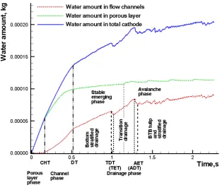
4.2.6 Amount of liquid water over time and the flooding phases

Based on the variation in the amount of liquid water over time in the porous layer, flow channels, and cathode, the liquid water flooding process inside of the cathode with the interdigitated design can be divided into three phases: the porous layer phase, in which the liquid water generated from the interface of the membrane and catalyst layer accumulates inside of the porous layer, the channel phase, in which the liquid water accumulates in the flow channels and the porous layer, and the drainage phase, in which the liquid water drains from the outlet channel.

The time for the porous layer phase can be defined as the time period from t = 0 to Cowboy Hat Time (CHT as defined in Fig. 4-10), i.e., the instant when the half-sine-wave shape begins to form the cowboy hat shape, as shown in Fig 4-6 (6). During this phase, no liquid water was inside of the flow channels, and the liquid water inside of the porous layer changed from a half-mango shape to a cowboy hat shape.

The time for the channel phase can be defined as the time period from CHT to the Departure Time (DT as defined in Fig. 4-10), which is the instant when the liquid water inside the outlet manifold begins to flow from the outlet channel. During this phase, the liquid water inside of the porous layer around the zones under the frames, which was initially shaped like a pancake (e.g., Fig 4-6 (3)), accumulated, as shown in Fig. 6(7). During this phase, the liquid water with a cowboy hat shape from the porous layer was subjected to an emerging process from the porous layer to the channels, which manifested itself as a Bunsen flame shape that developed from a “baby” (Fig 4-6 (7)) into an “adult” (Fig 4-6 (8)).

The drainage phase can be defined from DT onwards. The drainage phase of the porous layer can further be divided into two sub-phases: the stable emerging phase, which is the phase in which the liquid water from the porous layer enters the flow channels with a stable adult Bunsen-flame shape, and the avalanche phase in which the liquid water from the avalanche periodically and suddenly squeezes into, accumulates in, and squeezes out of the porous layer.

(55)

40

when the first BTB tulips flow out of the outlet channel, respectively. ADT and AET are defined as the instant when the water from the first avalanche reaches the outlet and the instant when the water flows out of the outlet channel, respectively.

Fig. 4‐10 Variation curve of the amount of water as a function of time in the entire domain

(CHT: Cowboy Hat time; DT: Departure Time; TDT: Tulip Departure Time; TET: Tulip Exit Time; ADT: Avalanche Departure Time; AET: Avalanche Exit Time)

(56)

41

From Fig. 4-10, the total amount of liquid water inside the cathode can be accounted for based on the above descriptions of the amount of liquid water in the porous layer and the flow channels.

4.3 Summary

In this study, the general liquid water flooding process inside of a DHFC cathode with an interdigitated design was investigated by analyzing the air-liquid interaction and by using the VOF method.

(1) The general process of liquid water flooding inside of this type of cathode begins from liquid water generation at the interface of the membrane and the catalyst layer and immediately moves inside of the porous layer based on the flow field design. Then, the liquid water begins to move into the flow channels and accumulates as it moves towards the outlet manifold. Finally, the water accumulates in the outlet manifold and drains through the outlet channel. This process can be classified into three phases: the porous layer phase, the channel phase, and the drainage phase, which is based on the Cowboy Hat Time and the Departure Time.

(2) During the liquid water flooding process, the liquid water can exhibit many different shapes such as a half-mango, half-dumbbell, half-sine-wave, cowboy hat, pancake, Bunsen flame, golden arch, BTB tulip, rivulet shape or a stratified flow pattern. The shape is the result of the interaction between the air and the liquid water as well as the flow geometries.