FAST NUMERICAL METHODS FOR BERNOULLI FREE BOUNDARY PROBLEMS∗
CHRISTOPHER M. KUSTER†, PIERRE A. GREMAUD†, AND RACHID TOUZANI‡
Abstract. The numerical solution of the free boundary Bernoulli problem is addressed. An iterative method based on a level-set formulation and boundary element method is proposed. Issues related to the implementation, the accuracy, and the generality of the method are discussed. The efficiency of the approach is illustrated by numerical results.
Key words. Bernoulli, free boundary, level set, boundary elements
AMS subject classifications. 65N38, 35R35, 76B99
DOI.10.1137/06065444X
1. Introduction. Bernoulli free boundary problems find their origin in the de-scription of free surfaces for ideal fluids [12]. There are, however, numerous other applications leading to similar formulations; see, for instance, [11]. For concreteness, we focus on the exterior Bernoulli problem. Let Ω be a bounded domain in R2. The exterior Bernoulli problem consists in seeking a bounded domain A⊃Ω and a functionudefined on ¯A\Ω such that
Δu= 0 inA\Ω, (1.1)
u= 1 on∂Ω, (1.2)
u= 0 on∂A, (1.3)
∂u
∂n=μ on∂A, (1.4)
where μ is given. In the previous example, one can think of uas a streamfunction and of Ω as an obstacle. Taking into account (1.3), condition (1.4) can be written as
| ∇u|=|μ| and corresponds, for fluid applications, to Bernoulli’s principle; see, for instance, [9].
The above problem has been extensively studied; see [11] for general remarks. For a convex simply connected bounded domain Ω, it is known that for any negative constantμ <0, the above problem admits a unique classical solution. Further, the free boundary ∂Ahas regularityC2,α; see [21, Theorem 1.1].1 The convexity assumption is necessary for uniqueness, as counterexamples show (see [11, Example 13]). The study of the interior Bernoulli problem is more delicate, and not even convexity can ensure uniqueness.
∗Received by the editors March 16, 2006; accepted for publication (in revised form) October 26,
2006; published electronically March 30, 2007.
http://www.siam.org/journals/sisc/29-2/65444.html
†Department of Mathematics and Center for Research in Scientific Computation, North Carolina
State University, Raleigh, NC 27695-8205 ([email protected], [email protected]). The work of the first author was partially supported by the National Science Foundation (NSF) through grant DMS-0244488. The work of the second author was partially supported by the NSF through grants DMS-0204578, DMS-0244488, and DMS-0410561.
‡Laboratoire de Math´ematiques, CNRS UMR 6620, Universit´e Blaise Pascal (Clermont-Ferrand),
63177 Aubi`ere Cedex, France ([email protected]).
1The result is, in fact, established in the more general case of thep-Laplacian in [21] and is generalized to nonconstantμin [22].
There are roughly two ways of tackling such problems numerically. First, a varia-tional formulation may be considered and the corresponding cost function minimized [19, 23, 28]; this requires the calculations of shape gradients. Second, a fixed point-type approach can be set up where a sequence of elliptic problems is solved in a sequence of converging domains, those domains being obtained through some updat-ing rule at each iteration [6, 11, 24]. The method studied in this paper falls in the latter category.
Two simple generic numerical tools are combined. First, the interface is repre-sented through a level-set formulation as described in section 2. Second, the elliptic part of the problem is solved through the use of a boundary element method; see section 3 (see [14] for another example of a method involving those two tools in a different setting). The proposed method is thus conceptually simpler than the shape optimization approach. Since it requires, in principle, only the calculations of quan-tities being defined on the interface or close to it, it is potentially faster than the finite difference approaches of, for instance, [6, 11, 24] or more generally of immersed interface-type methods [27]. The feasibility of the algorithm and its complexity are investigated in section 4.
A general overview of the strategy is as follows: the potential problem is solved with one of the conditions on the free boundary omitted, and then the omitted con-dition is used to update the location of the free boundary. More specifically, given an initial domain A0 ⊃ Ω, the simplest variant of this type consists in solving the¯ sequence of problems
Δuk= 0 in Ak\Ω, k= 0,1,2, . . . , (1.5)
uk= 1 on∂Ω, (1.6)
∂nuk=μ on∂Ak. (1.7)
For a given domain Ak, it is well known that problem (1.5)–(1.7) admits a unique solution; see, for instance, [15, Theorem 5.1]. The new domain Ak+1 is found by moving∂Ak in its normal direction so thatuk vanishes there. LetPk ∈∂Ak; to first order, we have
uk(Pk+1)≈uk(Pk) +μ dk,
wherePk+1=Pk+nkdk,nkbeing the outer unit normal to∂Ak atPk. The new point Pk+1, or similarly the distancedk, is determined by the requirementuk(Pk+1) = 0, i.e.,dk =−uk(Pk)
μ . The free boundary is thus updated according to 2
∂Ak+1=∂Ak−uk μ nk. (1.8)
2. Level-set representation of the interface. In the above iterative process, the interface∂Akhas to be updated as long as the residualuk|∂Akis not (numerically)
zero. Relation (1.8) indicates that the boundary should be moved in the normal direction by an amount proportional to the residual.
2The present iterative process can be modified by imposing the Neumann condition (1.7) on the “next” boundary∂Ak+1instead of∂Ak [11, 13]. However, in the formulation adopted here, those
If the residual is considered as a normal speed, a time-dependent problem can be set up for the “evolution” (or correction) of the domain Ak. We denote the domain so generatedAk(t) withAk(0) =Ak. LetF:R2→Rbe an extension of the residual away fromAk (see subsection 2.3 below). We want the interface Γ(t) =∂Ak(t) to be characterized by
Γ(0) =∂Ak, Γ(t) ={(x(t), t);x(0) =x0, x0∈∂Ak} fort >0, where
dx
dt =F n, x(0) =x0,
n being the unit outer normal to∂Ak(t). A level-set approach, as pioneered in [30] (see also [29, 34]), consists in representing the interface{Γ(t)}t≥0as the zero level set of family of level-set functions{φ(·, t)}t≥0 with the property
Ak(t) ={x∈R2;φ(x, t)<0}, Γ(t) =∂Ak(t) ={x∈R2;φ(x, t) = 0}, where Ak(t) denotes the domain stemming from the evolution of Ak through the above process. By taking the time derivative of the relationφ(x(t), t) = 0, the level-set equation is obtained:
∂tφ+F|∇φ|= 0, (2.1)
φ(·,0) =φ0, (2.2)
whereφ0 is a level-set function corresponding to∂Ak.
Several points related to the implementation of the above method now have to be considered. The fixed boundary∂Ω is approximated by a piecewise linear curve∂Ωh withN elements. The size of the smallest element of∂Ωhis denoted Δx. LetB⊂R2 be a square domain of size MΔx×MΔx, where M is chosen large enough so that B containsA. We associate with B, in a natural way, a uniform Cartesian meshBh of size Δx. In the following, the level-set functions are characterized by their nodal values on the meshBh. Two kinds of interpolation operators are considered onBh. In the contouring step (subsection 2.1), a classical P1 interpolation is used. In the projection step (subsection 2.2), a classical localQ2 interpolation is considered.
2.1. Contouring. In many applications of the level-set method, the actual re-construction of the interfaces is not needed. This is not the case here, as the elliptic problem (1.5)–(1.7) has to be solved in a family of successive domains defined by those interfaces. Letφbe a given level-set function andIPφitsP1-interpolant onBh. By contouring, we mean the operation that associates with the nodal values ofφthe zero level set ofIPφ. More precisely, each square cell of the underlying Cartesian grid is divided into two triangular elements,3 and on each of those triangles, the unique polynomial of degree 1 agreeing with the values of the level-set function at the vertices is considered. Contour lines are then constructed by connecting the zeros ofIPφon the grid lines. This process is facilitated by two facts: first, each triangle contains at most one contour line passing through it, and, second, the gradient ofIPφis piecewise constant on the grid elements, yielding an outward normal toAk(t). Note that both properties fail in general for the localQ2interpolant considered in the projection step below.
IfIPφis uniformly equal to zero on a given triangle, then the problem is under-resolved (Δxis too large) and the algorithm fails.
2.2. Projection. As mentioned above, some quantities such as the normal speed need to be extended away from the interface. The first step in this process consists again in an accurate reconstruction of the boundary. A loop through the mesh is done to determine which nodes are “close to” the interface. Here a node is close to the interface if it has a primary neighbor whereφhas opposite sign.
With each nodexi, we associate its eight closest neighbors and construct on this set of nine nodes the unique polynomial of degree 2 in each variable agreeing with the values of φ there. This local Q2 interpolant is denoted IQ,xiφ. For each node
xi close to the interface, the closest point x to xi on the zero level set of IQ,xiφis
computed. The square of the Cartesian distance, i.e.,|x−xi|2, is minimized subject to the constraintIQ,xiφ= 0. The Lagrangian for this problem is
L(x, λ) =|x−xi|2+λ IQ,xiφ(x).
(2.3)
To find the pointx, the system
∇x,λL(x, λ) = 0 (2.4)
is solved by Newton’s method with Armijo line search [25]. This projection method was introduced and discussed in [17]. It roughly corresponds to a simpler version of the method proposed in [8] which is based on cubic splines; see [26] for more comments and comparisons. The above algorithm can fail if the interface is underresolved.
The projection step could potentially be used to reconstruct the interface, i.e., as another contouring step. However, while it is locally more accurate than the above contouring algorithm (and is thus ideal when used in conjunction with the extension step described below), it has several disadvantages as a contouring tool (local character, nonconstant elementwise gradient).
2.3. Extension. This step extends the speed F away from the interface, so that (2.1), (2.2) can be solved. Let Γ be the interface obtained from the contouring step. By construction, Γ is a closed (for the problems considered here), possibly multiconnected, piecewise linear (on the triangular mesh derived from Bh) curve in B. The boundary nodes corresponding to Γ are denoted {ξj}; i.e., the ξj’s are the end points of the line segments that form Γ. Further, through the elliptic step (see section 3), the value of F at the center point of each linear segment of Γ is known; the center point nodes are denoted{ξ¯j}.
First, the values ofF at the midpoint boundary nodes{ξ¯j} are extended to the set of Cartesian nodes{xi}that form the vertices of the triangles containing the nodes
{ξj¯}.
More precisely, consider the node ¯ξj in Figure 1, left. This local extension step is based on the analysis of the “domain of influence” of the nodes{ξj¯}. This domain of influence is taken here as the set of all the points in B whose orthogonal projection on the line containing the segment through ¯ξj belongs to that segment. If a nodexi belongs to the domain of influence of ¯ξj, thenF is extended atxi by the valueF( ¯ξj) as in Figure 1, left. If instead the nodexiis in the domain of influence of more than one midpoint boundary node, as would be the case in the dark grey area in Figure 1, left, then the value at the midpoint of the closest segment toxi is retained. Finally, ifxi does not belong to the domain of influence of any midpoint boundary node, as in the light grey area in Figure 1, right, then the value ofF at xi is taken as
F(xj) = β
Fig. 1.Left: general view of the geometry involved in the local extension step and corresponding “domains of influence” (dark grey area: shock-like domain, light grey area: rarefaction-like domain); right: definition of the local anglesαandβ.
whereFj−1andFj are the values ofF at the midpoint boundary nodes ¯ξj−1 and ¯ξj, respectively, and where the anglesαandβare defined as in Figure 1, right. This way of defining the local extension ofF is compatible with the global extension (2.7).
Second, a renormalized function ˜φ is initialized as a signed distance function at the same Cartesian nodes at whichF has just been extended. The projection step is used to do this.
We emphasize that both of those local extension steps forF and ˜φtake place only on the nodes adjacent to the interface; the corresponding values are then used as start-ing points for the extension to the rest of the Cartesian nodes. This is accomplished using the fast marching method [2] to solve
| ∇φ˜|= 1 inB, (2.5)
˜
φ= 0 on Γ, (2.6)
∇F˜· ∇φ˜= 0 inB, (2.7)
˜
F =F on Γ. (2.8)
A fully upwind mixed first/second order discretization of the above equations is ap-plied on the meshBh; see [18, 35, 36] for more details.
2.4. Updating the interface. The interface is moved by updating the corre-sponding level-set function through (2.1), (2.2). More precisely, after the extension step, the level-set function ˜φ corresponding to the current interface Γ is a signed distance function, and, in particular,|∇φ˜|= 1. Therefore, (2.1), (2.2) here reads
∂tφ+ ˜F= 0,
φ(·,0) = ˜φ.
The update is then trivially computed by taking one forward Euler step,
where Δt=−2μ1 . Note that this corresponds to half the optimal time step given by (1.8); taking the “optimal” value from (1.8) may lead to overshoots in the position of the interface and may, in fact, result in slowing down the convergence of the global iterative process.
2.5. Initial interface. An initial guess of the interface’s position, ∂A0, needs to be provided. This can be done in an ad hoc way. In section 4, ∂A0 is taken as a curve of constant distance to Ω.
3. Boundary element method. Consider again the problem (1.5)–(1.7). For the sake of simplicity, the subscriptkis dropped in this section. We assume both∂A and∂Ω to be simple closed curves and let Γ =∂A∪∂Ω. The region of interestA\Ω¯ being interior to∂Aand exterior to∂Ω,∂Ais oriented counterclockwise, while∂Ω is clockwise.
Multiplying (1.5) by the fundamental solution G(x, y) := −2π1 log|x−y| and integrating twice by parts leads to
u(x) =
Γ
G(x, y) ∂u
∂ny(y)ds(y)−
Γ ∂G
∂ny(x, y)u(y)ds(y), (3.1)
where n is the unit outer normal to A\Ω at¯ y. The above integral representation is valid for x ∈ A\ Ω.¯ To treat the case x ∈ Γ, we define the linear operator
L:L2(Γ)→L2(Γ) by
Lv(x) = ⎧ ⎪ ⎪ ⎨ ⎪ ⎪ ⎩ v(x) 2 + ∂A ∂G
∂ny(x, y)v(y)ds(y)−
∂Ω
G(x, y)v(y)ds(y) forx∈∂A,
∂A ∂G
∂ny(x, y)v(y)ds(y)−
∂Ω
G(x, y)v(y)ds(y) forx∈∂Ω
and the functionF ∈L2(Γ) by
F(x) = ⎧ ⎪ ⎪ ⎨ ⎪ ⎪ ⎩ μ ∂A
G(x, y)ds(y)−
∂Ω ∂G
∂ny(x, y)ds(y) forx∈∂A,
μ
∂A
G(x, y)ds(y)−
∂Ω ∂G
∂ny(x, y)ds(y)−
1
2 forx∈∂Ω.
Taking into account the boundary conditions (1.6) and (1.7), it is then standard to check that if
w(x) =
u(x) forx∈∂A, ∂u
∂n(x) forx∈∂Ω, whereuis the solution to (1.5)–(1.7), then
Lw(x) =F(x) ∀x∈Γ. (3.2)
Problem (3.2) is discretized as follows. The interface ∂A = ∂Ah is obtained through contouring of a given level-set function, see section 2, and piecewise constant elements are considered. The functionwsolution to (3.2) is approximated bywhsuch that
whereeis an edge of either∂Ahor∂Ωhand whereweis the constant value ofwh on that edge. Equation (3.2) is then collocated at the midpoints of the edges. In other words, for a generic piecewise constant functionvh, we define
Lhvh( ¯ξe) =
⎧ ⎪ ⎪ ⎪ ⎪ ⎪ ⎪ ⎪ ⎪ ⎪ ⎨ ⎪ ⎪ ⎪ ⎪ ⎪ ⎪ ⎪ ⎪ ⎪ ⎩
vh( ¯ξe)
2 +
∂Ah
∂G
∂ny( ¯ξe, y)vh(y)ds(y)−
∂Ωh
G( ¯ξe, y)vh(y)ds(y)
for ¯ξe∈∂Ah,
∂Ah
∂G
∂ny( ¯ξe, y)vh(y)ds(y)−
∂Ωh
G( ¯ξe, y)vh(y)ds(y)
for ¯ξe∈∂Ωh,
where ¯ξeis the midpoint of the edgee. Similarly, we also have
Fh( ¯ξe) =
⎧ ⎪ ⎪ ⎪ ⎨ ⎪ ⎪ ⎪ ⎩ μ ∂Ah
G( ¯ξe, y)ds(y)−
∂Ωh
∂G
∂ny( ¯ξe, y)ds(y) for ¯ξe∈∂Ah,
μ
∂Ah
G( ¯ξe, y)ds(y)−
∂Ωh
∂G
∂ny( ¯ξe, y)ds(y)−
1
2 for ¯ξe∈∂Ωh.
The approximate solutionwh is the solution to
Lhwh( ¯ξe) =Fh( ¯ξe) ∀ξe¯ ∈∂Ah∪∂Ωh. (3.3)
The above integrals are computed exactly in the present implementation, in the sense of the Cauchy principal value where appropriate; see [4] for more details.
Both the integral equation (3.2) and the linear problem (3.3) are well conditioned with one exception: 0 is an eigenvalue of L if and only if the transfinite diameter of A is 1 [20]. This can be avoided by appropriate rescaling if necessary. It can be verified thatLhadmits eigenvalues and singular values that are bounded independent of the mesh; see, e.g., [20] or [31] for explicit expressions of the eigenvalues in some specific cases. Further, in spite of the fact that the elements of ∂Ah are allowed to be arbitrarily small, the condition number ofLh has been numerically verified to be of order N, which would correspond to the uniform mesh case [3]. The condition number of the matrices corresponding to the numerical tests of section 4 are on the order of 100. The resulting linear system is solved by GMRES [25, 33], which is consequently expected to perform well here even without preconditioning; see also [7] for a general convergence result for GMRES applied to integral equations. GMRES is restarted after 20 steps (i.e., the solver is GMRES(20)) and is stopped on small relative residuals; more precisely, the stopping criterion is
Fh− Lhw2≤10−10Fh2,
where wdenotes the current iterate. With the above parameters, GMRES has been observed to perform slightly better than other CG-like methods such as QMR and Bi-CGSTAB [25] on the test problems of section 4.
4. Numerical results.
Input: a discretization of the boundary∂Ω,∂Ωh, μ Create the underlying Cartesian gridBh
Create a level set functionφonBh corresponding to∂A0 k= 0
R−1= 1010 (initial residual)
loop
Contourφ(subsection 2.1) to find∂Ak Solve (3.3) to getu
Rk = max of|u|on∂Ak
if(Rk−1−Rk)/Rk <10−3(small residual decrease)then STOP
end if
SetF =uon∂Ak
ExtendφandF (subsections 2.2 and 2.3) Move boundary (subsection 2.4)
k=k+ 1
end loop
Several remarks are in order.
• Profiling reveals that for reasonable meshes the relative costs of contouring and interface updating are very low (less than 1%), while most of the time is spent constructing and solving the linear system (3.3) (about 90%) and extending the solution (about 10%). Methods such as fast multipoles [5, 32] can be used to bring down the asymptotic complexity of the linear solver fromO(N2) toO(N), whereN is the number of elements of∂Ω
h. However, this results in increased efficiency only for very large values of N; see [26, Appendix] for more details; see also [16] for a large-scale two-dimensional ex-ample. Fast summation methods should be considered for three-dimensional problems.
• Progressive mesh refinement can be considered; i.e., a coarse mesh solution can be used as the starting point. A strategy of this type is, for instance, used in [23] for a similar type of problem but for a different numerical approach.
• In solving (3.3), the “missing” condition (1.3) can be used when choosing the initial iterate for GMRES. This results in faster convergence (fewer GMRES iterates) as the algorithm progresses.
• The extension step through fast marching (subsection 2.3) is done in the whole computational domain B. The corresponding complexity is O(M2logM), where M2 is the total number of nodes in the Cartesian gridBh. A narrow band/computational tube implementation [2, 37] could be considered to speed up the algorithm. However, the global complexity of the problem would not change: if the width of the band is a constant multiple of Δx, saynΔx, then by (2.9), Δt should be reduced from −1
2μ to a value less than nΔx
|F˜| since the band has to contain the boundary.
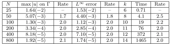
Table 1
Convergence and complexity rates for Example 1 (radial case); N is number of elements on
∂Ωh,L∞ error refers to the Hausdorff distance between exact and computed boundaries,kis the number of nonlinear iterations (see section4.1), Time is the runtime in seconds.
N max|u|on Γ Rate L∞error Rate k Time Rate 25 1.64(−2) – 1.53(−2) – 6 0.71 – 50 5.07(−3) 1.7 4.40(−3) 1.8 8 4.1 2.5 100 1.30(−3) 2.0 1.12(−3) 2.0 10 19 2.2 200 3.34(−4) 2.0 2.85(−4) 2.0 11 76 2.0 400 8.18(−5) 2.0 7.10(−5) 2.0 12 372 2.1 800 1.92(−5) 2.1 1.74(−5) 2.0 14 1465 2.0
• The use of second order fast marching is not crucial for the accuracy of the method which is dictated by both the contouring and boundary element methods. It was observed that first order fast marching may lead to more iterations (domain updates), and, hence, due to the very little difference in cost per iteration, the use of second order fast marching is advocated.
• The numerical solutions are observed to be remarkably independent of the initial domain∂A0(for problems with unique solutions [11]). More iterations can be expected in case of poor initial guesses (for instance if the smoothness properties of∂A0 are vastly different from those of∂A).
4.2. Example 1. Following [11], a quick look at the radial case is instructive. Let Ω be the unit ball. We consider the problem (1.1)–(1.4) with Ω as above and μ=−2. The solution to (1.1)–(1.3) withAbeing the ball of radiusRcentered at the origin is
u(r) =−2Rlogr+ 1,
expressed in polar coordinates. An iterative process similar to the one above can then be considered. Taking (1.8) into account, thekth step of the algorithm reads
Rk+1=Rk−RklogRk+ 1
2, k= 1,2, . . . .
Therefore, in the fully radial case, the problem amounts to finding a fixed point to the function f(R) = R−RlogR+ 1
2. The function f has a unique fixed point ¯R, where
¯
R= 1
2W(12),
the functionW being the Lambert W function4 [10].
Table 1 shows second order convergence in the L∞ norm. Full second order convergence is obtained even though the elliptic solver is based on a piecewise constant discretization. This is due to the fact that the exact solution is constant on both the inner and outer boundaries. Further, when measured with respect to runtime, the complexity is also second order.
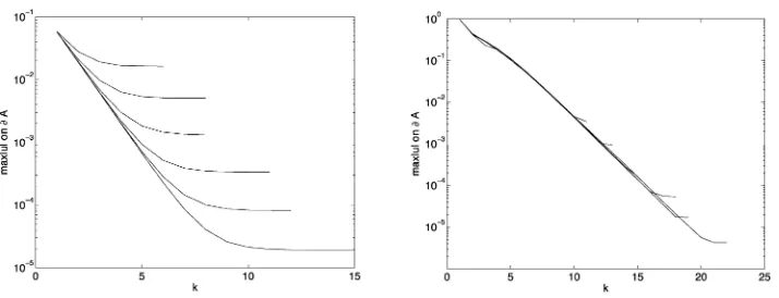
The convergence history is instructive. Figure 2, left, displays the error (maximum of|u|on the free boundary) through the iterations. The behavior of the first iterates is governed by the geometry, see (2.9), and is only weakly dependent on the mesh size
Fig. 2. Convergence history of the iterations: maximum value of |u|on the current interface as a function of the iteration number; left: Example 1, right: Example2. The convergence curves are in the obvious order: from top to bottom,N= 25,50,100,200,400,800.
Δx. The later iterations during which the fine structure of the boundary is determined do depend on Δx. This explains the mesh dependency of the number of iterations observed in Table 1.
4.3. Example 2. We consider here the problem (1.1)–(1.4) with Ω consisting of two disks of radius 1, one centered at (−2,2) and one at (2,−2); further, μ=−1/4. The initial boundary is taken as two circles of radius 1.1, one around each of the inner disks. Note that for this choice of μ, the exact boundary is simply connected. A couple of iterates are displayed in Figure 3. One can note that after the first step the correct topology of the interface has already been achieved.
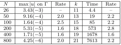
No exact solution is available for the present example. In Table 2, the maximum of u on the boundary is reported. By construction, this maximum should vanish for the converged solution. The complexity, as measured from the runtimes, is also reported. In both cases, the rates are about two.
Convergence history is displayed in Figure 2, right; a behavior similar as that of Example 1 is observed.
5. Conclusion. Solutions of the Bernoulli free boundary problem can be effi-ciently computed by the method presented here. Providing a Green’s function is available, the method can be used to solve other free boundary problems. For in-stance, it can be applied with only minor modifications to the Prandtl–Batchelor problem (see [1] and the references therein), which consists in looking for a domainA which is now interior to the fixed domain Ω such that for a given functionσ,
|∇uA|2− |∇uΩ|2=σ on∂A,
whereuAand uΩsolve
ΔuA=−ω in A, uA= 0 on∂A,
⎧ ⎪ ⎨ ⎪ ⎩
ΔuΩ= 0 in Ω,
uΩ= 0 on∂A,
uΩ=μ on∂Ω,
μandω being positive constants.5
5To avoid the calculation of a bulk due to the inhomogeneity, a particular solution to Δu 0=−ω (for instanceu0=−ω4(x2+y2)) can easily be subtracted fromuA. This restores homogeneity but
Fig. 3.Evolution of the interface for Example 2at the initial step and after steps1,2, and15 (N= 100).
Table 2
Convergence and complexity rates for Example 2; N is number of elements on∂Ωh,k is the number of nonlinear iterations (see section4.1), Time is the runtime in seconds.
N max|u|on Γ Rate k Time Rate 26 3.43(−3) – 11 4.4 – 50 9.16(−4) 2.0 13 19 2.2 100 1.64(−4) 2.5 15 85 2.2 200 5.31(−5) 1.6 18 573 2.8 400 1.71(−5) 1.6 19 1678 1.6 800 4.25(−6) 2.0 21 7613 2.2
REFERENCES
[1] A. Acker,On the existence of convex solutions to a generalized Prandtl-Batchelor free bound-ary problem-II, Z. Angew. Math. Phys., 53 (2002), pp. 438–485.
[3] M. Ainsworth, W. McLean, and T. Tran,The conditioning of boundary element equations on locally refined meshes and preconditioning by diagonal scaling, SIAM J. Numer. Anal., 36 (1999), pp. 1901–1932.
[4] K. E. Atkinson,The Numerical Solutions of Integral Equations of the Second Kind, Cambridge
Monogr. Appl. Comput. Math. 4, Cambridge University Press, Cambridge, UK, 1997. [5] R. Beatson and L. Greengard, A short course on fast multipole methods, in Wavelets,
Multilevel Methods and Elliptic PDEs (Leicester, 1996), Numer. Math. Sci. Comput., Oxford University Press, New York, 1997, pp. 1–37.
[6] F. Bouchon, S. Clain, and R. Touzani,Numerical solution of the free boundary Bernoulli problem using a level set formulation, Comput. Methods Appl. Mech. Engrg., 194 (2005), pp. 3934–3948.
[7] S. L. Campbell, I. C. F. Ipsen, C. T. Kelley, C. D. Meyer, and Z. Q. Xue,Convergence estimates for solution of integral equations with GMRES, J. Integral Equations Appl., 8 (1996), pp. 19–34.
[8] D. L. Chopp,Some improvements of the fast marching method, SIAM J. Sci. Comput., 23
(2001), pp. 230–244.
[9] A. J. Chorin and J. E. Marsden,A Mathematical Introduction to Fluid Mechanics, Springer,
New York, 1992.
[10] R. M. Corless, G. H. Gonnet, D. E. G. Hare, D. J. Jeffrey, and D. E. Knuth,On the LambertW function, Adv. Comput. Math., 5 (1996), pp. 329–359.
[11] M. Flucher and M. Rumpf,Bernoulli’s free-boundary problem, qualitative theory and nu-merical approximation, J. Reine Angew. Math., 486 (1997), pp. 165–204.
[12] K. O. Friedrichs, Uber ein Minimumproblem f¨¨ ur Potentialstr¨omungen mit freiem Rand,
Math. Ann., 109 (1934), pp. 60–82.
[13] P. R. Garabedian, Calculation of axially symmetric cavities and jets, Pacific J. Math., 6
(1956), pp. 611–684.
[14] M. Garzon, D. Adalsteinsson, L. Gray, and J. A. Sethian,A coupled level set-boundary integral method for moving boundary simulations, Interfaces Free Bound., 7 (2005), pp. 277–302.
[15] R. Gonz´alez and R. Kress,On the treatment of a Dirichlet–Neumann mixed boundary value problem for harmonic functions by an integral equation method, SIAM J. Math. Anal., 8 (1977), pp. 504–517.
[16] A. Greenbaum, L. Greengard, and G. B. McFadden,Laplace’s equation and the Dirichlet-Neumann map in multiply connected domains, J. Comput. Phys., 105 (1993), pp. 267–278. [17] P. A. Gremaud, C. M. Kuster, and Z. Li,A study of numerical methods for the level set
approach, Appl. Numer. Math., to appear.
[18] P. A. Gremaud and C. M. Kuster,Computational study of fast methods for the eikonal equation, SIAM J. Sci. Comput., 27 (2006), pp. 1803–1816.
[19] J. Haslinger, T. Kozubek, K. Kunisch, and G. Peichl,Shape optimization and fictitious domain approach for solving free-boundary problems of Bernoulli type, Comput. Optim. Appl., 26 (2003), pp. 231–251.
[20] J. Hayes and R. Kellner,The eigenvalue problem for a pair of coupled integral equations arising in the numerical solution of Laplace’s equation, SIAM J. Appl. Math., 22 (1972), pp. 503–513.
[21] A. Henrot and H. Shahgholian,Existence of classical solutions to a free boundary problem for thep-Laplace operator.I.The exterior convex case, J. Reine Angew. Math., 521 (2000), pp. 85–97.
[22] A. Henrot and H. Shahgholian,The one phase free boundary problem for thep-Laplacian with non-constant Bernoulli boundary condition, Trans. Amer. Math. Soc., 354 (2002), pp. 2399–2416.
[23] K. Ito, K. Kunisch, and G. H. Peichl,Variational approach to shape derivatives for a class of Bernoulli problems, J. Math. Anal. Appl., 314 (2006), pp. 126–149.
[24] K. T. K¨arkk¨ainen and T. Tiihonen,Free surfaces: Shape sensitivity analysis and numerical methods, Internat. J. Numer. Methods Engrg., 44 (1999), pp. 1079–1098.
[25] C. T. Kelley,Iterative Methods for Linear and Nonlinear Problems, Frontiers Appl. Math.
16, SIAM, Philadelphia, 1995.
[26] C. M. Kuster,Fast Numerical Methods for Evolving Interfaces, Ph.D. thesis, Department of
Mathematics, North Carolina State University, Raleigh, NC, 2006; http://www.lib.ncsu. edu/theses/available/etd-04262006-083221/.
[27] Z. Li and K. Ito,The Immersed Interface Method: Numerical Solutions of PDEs Involving Interfaces and Irregular Domains, Frontiers Appl. Math. 33, SIAM, Philadelphia, 2006. [28] G. Mejak,Numerical solution of Bernoulli-type free boundary value problems by variable
[29] S. J. Osher and R. P. Fedkiw,Level Set Methods and Dynamic Implicit Surfaces, Appl.
Math. Sci. 153, Springer, New York, 2002.
[30] S. Osher and J. Sethian,Fronts propagating with curvature dependent speed: Algorithms based on Hamilton-Jacobi formulations, J. Comput. Phys., 56 (1988), pp. 12–49. [31] G. J. Rodin and O. Steinbach,Boundary element preconditioners for problems defined on
slender domains, SIAM J. Sci. Comput., 24 (2003), pp. 1450–1464.
[32] V. Rokhlin,Rapid solution of integral equations of classical potential theory, J. Comput. Phys.,
60 (1983), pp. 187–207.
[33] Y. Saad and M. H. Schultz,GMRES: A generalized minimal residual algorithm for solving nonsymmetric linear systems, SIAM J. Sci. Statist. Comput., 7 (1986), pp. 856–869. [34] J. A. Sethian,Level Set Methods and Fast Marching Methods, Cambridge University Press,
Cambridge, UK, 1999.
[35] J. A. Sethian and A. Vladimirsky,Fast methods for the Eikonal and related Hamilton-Jacobi equations on unstructured meshes, Proc. Natl. Acad. Sci. USA, 97 (2000), pp. 5699–5703. [36] J. A. Sethian and A. Vladimirsky, Ordered upwind methods for static Hamilton–Jacobi
equations: Theory and algorithms, SIAM J. Numer. Anal., 41 (2003), pp. 325–363. [37] L. Yatziv, A. Bartesaghi, and G. Sapiro,O(N) implementation of the fast marching