Individual-Based Modeling and Nonlinear Analysis for Complex Systems with Application to Theoretical Ecology

(1)

University of Windsor University of Windsor

Scholarship at UWindsor

Electronic Theses and Dissertations Theses, Dissertations, and Major Papers

2014

Individual-Based Modeling and Nonlinear Analysis for Complex

Systems with Application to Theoretical Ecology

Abbas Ghadri Golestani

University of Windsor

Follow this and additional works at: https://scholar.uwindsor.ca/etd

Recommended Citation Recommended Citation

Ghadri Golestani, Abbas, "Individual-Based Modeling and Nonlinear Analysis for Complex Systems with Application to Theoretical Ecology" (2014). Electronic Theses and Dissertations. 5253.

https://scholar.uwindsor.ca/etd/5253

This online database contains the full-text of PhD dissertations and Masters’ theses of University of Windsor students from 1954 forward. These documents are made available for personal study and research purposes only, in accordance with the Canadian Copyright Act and the Creative Commons license—CC BY-NC-ND (Attribution, Non-Commercial, No Derivative Works). Under this license, works must always be attributed to the copyright holder (original author), cannot be used for any commercial purposes, and may not be altered. Any other use would require the permission of the copyright holder. Students may inquire about withdrawing their dissertation and/or thesis from this database. For additional inquiries, please contact the repository administrator via email

(2)

Individual-Based Modeling and Nonlinear Analysis

for Complex Systems with Application to Theoretical

Ecology

By

Abbas Ghadri Golestani

A Dissertation

submitted to the Faculty of Graduate Studies through the Department of Computer Science in Partial Fulfillment of the Requirements for

the Degree of Doctor of Philosophy at the University of Windsor

Windsor, Ontario, Canada 2014

(3)

Individual-Based Modeling and Nonlinear Analysis for Complex Systems with Application to Theoretical Ecology

by

Abbas Ghadri Golestani

APPROVED BY:

___________________________________________ Dr. J. Liu, External Examiner

Hong Kong Baptist University

______________________________________________ Dr. D. Heath

Great Lakes Institute for Environmental Research

______________________________________________ Dr. B. Boufama

School of Computer Science

______________________________________________ Dr. Z. Kobti

______________________________________________ Dr. R. Gras, Advisor

(4)

iii

Declaration of Co-Authorship / Previous Publication

I. Co-Authorship Declaration

I hereby declare that this dissertation incorporates material thatis result of joint research

with Dr. Robin Gras, my supervisor. This dissertation also incorporates the outcome of a joint

research undertaken in collaboration with Dr. M. Cristescu and Dr. A.P Hendy under the

supervision of professor Robin Gras. The collaboration is covered in Chapter 4 of the

dissertation. In all cases, the key ideas, primary contributions, experimental designs, data analysis

and interpretation, were performed by the author, and the contribution of co-author was primarily

through the provision of required background biological information. In Chapter 3, Ms. Khater

also contributed in explaining the materials.

I am aware of the University of Windsor Senate Policy on Authorship and I certify that I

have properly acknowledged the contribution of other researchers to my dissertation, and have

obtained written permission from each of the co-author(s) to include the above material(s) in my

dissertation.

I certify that, with the above qualification, this dissertation, and the research to which it

refers, is the product of my own work.

II. Declaration of Previous Publication

(5)

iv

Dissertation Chapter

Publication title/full citation Publication

status*

Chapter 2 R. Gras, A. Golestani, M. Hosseini, M. Khater, Y.M. Farahani, M. Mashayekhi, M. Sina, A. Sajadi, E. Salehi and R. Scott, EcoSim: an individual-based platform for studying evolution, European Conference on Artificial Life, pp 284-286, 2011.

Published

Chapter 2 M. Mashayekhi, A. Golestani, Y.M. Farahani, R. Gras, An enhanced artificial ecosystem: Investigating emergence of ecological niches, International Conference on the Simulation and Synthesis of Living Systems (ALIFE 14), pp 693-700, 2014.

Published

Chapter 4 A. Golestani, R. Gras, and M. Cristescu, Speciation with gene flow in a heterogeneous virtual world: can physical obstacles accelerate speciation?,

Proceedings of the Royal Society B: Biological Sciences, vol. 279 no. 1740,

pp 3055-3064, 2012.

Published

Chapter 4 A. Golestani, R. Gras, A New Species Abundance Distribution Model Based on Model Combination, International Journal of Biostatistics (IJB), 9(1): 1–

16, 2013.

Published

Chapter 4 A. Golestani, R. Gras, Using Machine Learning Techniques for Identifying Important Characteristics to Predict Changes in Species Richness in EcoSim, an Individual-Based Ecosystem Simulation", International Conference on Machine Learning and Data Analysis (ICMLDA'12), vol 1, pp 465-470, San Francisco, 2012.

Published

Chapter 4 R. Gras, A. Golestani, M. Cristescu, and A.P. Hendry, Speciation without pre-defined fitness functions, PLOS ONE, 2014.

Submitted

Chapter 5 A. Golestani, R. Gras, Regularity Analysis of an individual-based Ecosystem Simulation, journal of Chaos: An Interdisciplinary journal of Nonlinear Science, CHAOS 20, 043120. pp 1-13, 2010.

Published

Chapter 5 A. Golestani, R. Gras, Identifying Origin of Self-Similarity in EcoSim, an Individual-Based Ecosystem Simulation, Using Wavelet-based Multifractal Analysis, International Conference on Modeling, Simulation and Control (ICMSC'12), vol 2, pp 1275-1282, San Francisco, 2012.

Published

Chapter 5 Y.M. Farahani, A. Golestani, R. Gras, Complexity and Chaos Analysis of a Predator-Prey Ecosystem Simulation, COGNITIVE, ISBN: 978-1-61208-001-7, pp: 52-59, 2010.

Published

Chapter 5 A. Golestani, R. Gras, "Multifractal Phenomena in EcoSim, a Large Scale Individual-Based Ecosystem Simulation", ICAI (International Conference on

(6)

v

Artificial Intelligence), Las Vegas, USA, pp 991-999, 2011.

Chapter 6 A. Golestani, R.Gras, Can We Predict the Unpredictable?, Scientific Reports 4, 6834; DOI:10.1038/srep068342014.

Published

Chapter 6 A. Golestani, R. Gras, System and Process for Predictive Chaos Analysis , Filed under US Patent Application Serial Number 61/882863.

In press

Chapter 6 A. Golestani, R. Gras, Method And Apparatus For Prediction Of Epileptic Seizures, Filed under US Patent Application Serial Number 62/042535.

In press

I certify that I have obtained a written permission from the copyright owner(s) to include the above published material(s) in my dissertation. I certify that the above material describes work completed during my registration as graduate student at the University of Windsor.

I declare that, to the best of my knowledge, my dissertation does not infringe upon anyone’s copyright nor violate any proprietary rights and that any ideas, techniques, quotations, or any other material from the work of other people included in my dissertation, published or otherwise, are fully acknowledged in accordance with the standard referencing practices. Furthermore, to the extent that I have included copyrighted material that surpasses the bounds of fair dealing within the meaning of the Canada Copyright Act, I certify that I have obtained a written permission from the copyright owner(s) to include such material(s) in my dissertation.

(7)

vi

ABSTRACT

One approach to understanding the behaviour of complex systems is individual-based modeling,

which provides a bottom-up approach allowing for the consideration of the traits and behaviour of

individual organisms. Ecosystem models aim to characterize the major dynamics of ecosystems,

in order to synthesize the understanding of such systems and to allow predictions of their

behaviour. Moreover, ecosystem simulations have the potential to help scientists address

theoretical questions as well as helping with ecological resource management. Because in reality

biologists do not have much data regarding variations in ecosystems over long periods of time,

using the results of ecological computer simulation for making reasonable predictions can help

biologists to better understand the long-term behaviour of ecosystems. Different versions of

ecosystem simulations have been developed to investigate several questions in ecology such as

how speciation proceeds in the absence of experimenter-defined functions. I have investigated

some of these questions relying on complex interactions between the many individuals involved

in the system, as well as long-term evolutionary patterns and processes such as speciation and

macroevolution.

Most scientists now believe that natural phenomena have to be looking as a chaotic system. In

the past few years, chaos analysis techniques have gained increasing attention over a variety of

applications. I have analyzed results of complex models to see whether chaotic behaviour can

emerge, since any attempt to model a realistic system needs to have the capacity to generate

patterns as complex as the ones that are observed in real systems. To further understand the

complex behaviour of real systems, a new algorithm for long-term prediction of time series

behaviour is also proposed based on chaos analysis. We evaluated the performance of our new

method with respect to the prediction of the Dow-Jones industrial index time series, epileptic

(8)

vii

DEDICATION

To my parents for the courage

To my wife for the patience

(9)

viii

ACKNOWLEDGEMENTS

I would like to gratefully thank Dr. Robin Gras my supervisor, for giving me the opportunity and

continued guidance to apply and extend my knowledge in a cross disciplinary field, working at

the forefront of computer science. I would like to thank my committee members Dr. Liu, Dr.

Heath, Dr. Boufama and Dr. Kobti for accepting to allocate part of their valuable time to evaluate

my research.

This work was made possible by the facilities of Shared Hierarchical Academic Research

(10)

ix

List of Tables

Table 2-1. Several physical and life history characteristics of individuals from 10 independent EcoSim runs. ... 16 Table 2-2. Values for user-specified parameters in EcoSim. ... 27 Table 2-3. The initial parameters of the EcoSim at the first time step of the simulation. There are 42 parameters for each run of EcoSim. The value of these parameters has been obtained

empirically and by biologists' expert opinion to preserve the equilibrium in the ecosystem. ... 30 Table 2-4. Initial FCM values for Prey (See Table 2-5). Every prey individual has a FCM which represent its behaviour. At first time step, all prey individuals have an initial FCM. During time and during each generation with operators like crossover and mutation, the FCM of individuals change. ... 31 Table 2-5. Prey/predator FCM abbreviation table. The abbreviation used to present concepts of FCM in EcoSim. These abbreviations have been used in other tables to show values of these concepts. ... 31 Table 2-6. Parameters of prey defuzzification function (see Figure 2-5). The function that has been used for fuzzifications uses three parameters which shape the fuzzification curve. ... 32 Table 2-7. Initial FCM for Predator (See Table 2-5). Every predator individual has a FCM which represent its behaviour. At first time step, all predator individuals have an initial FCM. During time and during each generation with operators like crossover and mutation, the FCM of

individuals change ... 33 Table 2-8. Parameters of predator defuzzification function (see Figure 2-5). The function that has been used for fuzzifications uses three parameters which shape the fuzzification curve. ... 34 Table 4-1.Average and standard deviation of the number and size of spirals in 30 independent runs of every configuration. ... 68 Table 4-2. Average and standard deviation of the number of species in the 30 independent runs for every configuration ... 69 Table 4-3. The average and standard deviation of individuals' average distances around the spatial center of the species in the 30 independent runs corresponding to the 3 speciation thresholds for the 3 configurations. ... 71 Table 4-4. The median of maximum distances between individuals around the center of species in the 30 independent runs corresponding to the 3 speciation thresholds for the 3

(16)

xv

Table 4-6. Several physical and life history characteristics of individuals averaged over 10 independent runs for every experiment. Exp1 stands for Selection, Enforced Reproductive Isolation, and Low Dispersal, Exp2 for Selection and Low Dispersal, Exp3 for Selection and High Dispersal, Exp4 for No Selection and High Dispersal and Exp5 for No Selection and Low Dispersal. In the experiments without natural selection, because there is no behavioural model, some characteristics do not exist. ... 80 Table 4-7. Different families of SADs. ... 90 Table 4-8. Interpretation of weights in three sub-range combinations for four base models ... 97 Table 4-9. Characteristics of different real datasets from nature (S: Number of Species, N:

Number of Individuals). ... 101 Table 4-10. Different errors of the four selected models over eight various datasets. FPLP models is trained over the Fushan dataset ... 102 Table 4-11. The average percentage of improvement of FPLP method compared to other

methods in various measures in the case of using "Fushan" dataset as a training data set. ... 105 Table 4-12. The p-value for the distance between error rates of different models for each

measure in the case of using "Fushan" dataset as a training data set. ... 105 Table 4-13. Different errors of the four selected models over eight various datasets. Models trained over Malaysian butterflies dataset. ... 106 Table 4-14. The average percentage of improvement of FPLP compared to each measure in the case of using "Malaysian butterflies" dataset as a training data set. ... 108 Table 4-15. The p-value for the distance between error rates of different models for each

measure in the case of using "Malaysian butterflies" dataset as a training data set. ... 109 Table 4-16. Results of prediction of species richness for next 100 time steps by decision tree on training set. ... 115 Table 4-17. Results of prediction of species richness for next 100 time steps by decision tree on test set. ... 116 Table 6-1. Comparison of mean absolute percentage error (MAPE) [300] between several

(17)

(18)

xvii

List of Figures

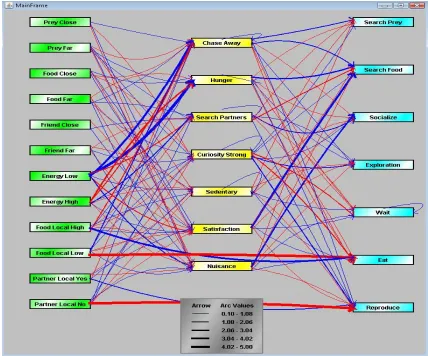
Figure 2-1. A sample of a predator’s FCM including concepts and edges. The width of each edge shows the influence value of that edge. Color of an edge shows inhibitory (red) or excitatory

(blue) effects. ... 19

Figure 2-2. An FCM for detection of foe (predator) and decision to evade, with its corresponding matrix (0 for ‘Foe close’, 1 for ‘Foe far’, 2 for ‘Fear’ and 3 for ‘Evasion’) and the fuzzification and defuzzification functions [91]. ... 21

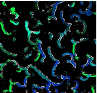
Figure 2-3. A snapshot of the virtual world in one specific time step, white color represents predator species and the other colors show different prey species. ... 22

Figure 2-4. An FCM for detection of foe (predator) - difference between perception and sensation [91]. This map shows different kind of interactions between three kinds of concepts: perception concept (Foe close and Foe far), internal concept (Fear) and motor concept (Evasion). ... 24

Figure 2-5. The three parameters that specify the shape of the curve. The first parameter specifies the center of curve in the horizontal axis, the second parameter specifies the lower band of curve in the vertical axis and the third parameter specifies the width of curve. ... 33

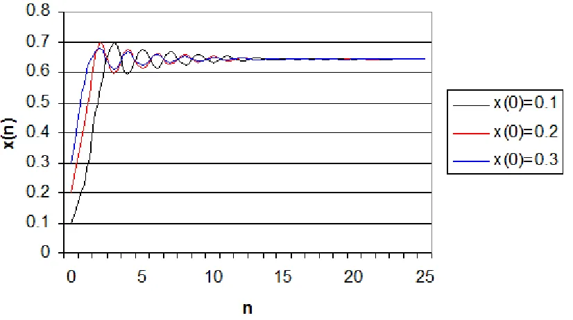
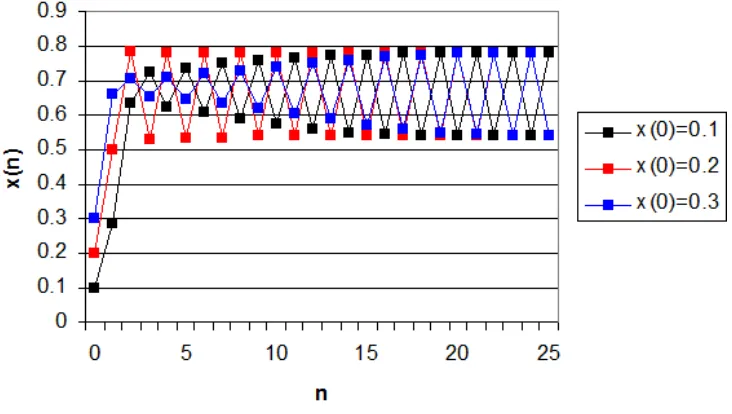
Figure 3-1. Logistic Map with a = 2.8. The population will eventually stabilize. ... 38

Figure 3-2. Logistic Map with a = 3.2. The population oscillate between two points. ... 39

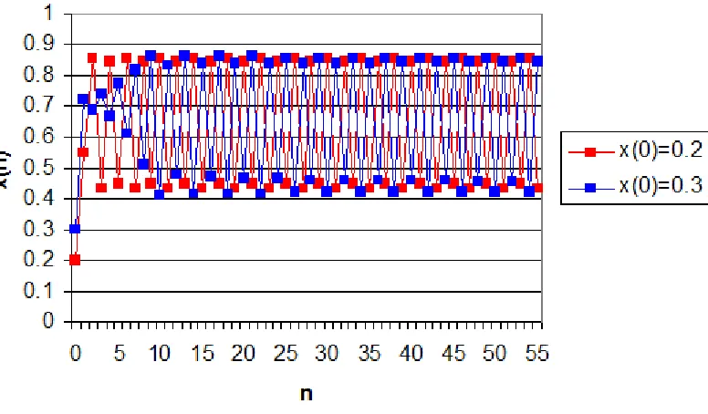
Figure 3-3. Logistic Map with a = 3.5. The population oscillate between four points. ... 40

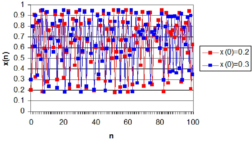
Figure 3-4. Logistic Map with a = 3.8. The behaviour of population is non-periodic, bounded and deterministic (chaotic). ... 41

Figure 3-5. The Koch curve illustrates self-similarity. As the image is enlarged, the same pattern re-appears. ... 45

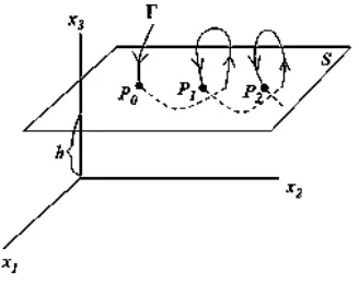
Figure 3-6. Intersection between the flow (Γ) and the Poincaré section (S) generating the set of points P = (P0, P1, P2). ... 52

Figure 3-7. Intersection of Lorenz attractor and Poincaré section. The Poincaré map is product of this stage. ... 53

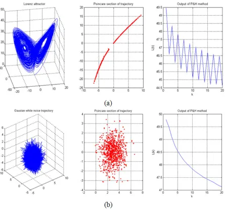
Figure 3-8. Applying of P&H method over Lorenz time series and random time series. ... 55

(19)

xviii

Figure 4-1. Computation of final direction of the escape route for prey. The prey agent takes into account the position of the closest obstacle as well as the position of the predators and the shortest path (path#1) is used to avoid another obstacles (red line). ... 66 Figure 4-2. An overview of the distribution of species and populations in the world with density of obstacles (10%) and the density of obstacles (0%) experiment. (a) View of the whole world in the density of obstacles (0%) experiment. (b) Magnified part of the world in density of obstacles (0%) experiment. (c) View of the entire world with obstacles. (d) Magnified part of the world with obstacles. The blue squares are obstacle cells and dots are individuals. Different colored dots represent different prey species and white dots represent predator species. ... 67 Figure 4-3. Comparison between numbers of prey species in the whole world during 16,000 time steps. Every curve represents an average value obtained from 30 independent runs with three different speciation thresholds. ... 69 Figure 4-4. Percentage of prey individuals that fail in reproduction action (a,c) and socialize action (b,d) between the various density of obstacles (1%, 10%) configuration and the density of obstacles (0%) configurations. The red curves represent the density of obstacles (0%)

experiment and the blue curves represent the experiments with various densities of obstacles (1%, 10%). Every curve is an average value obtained from 30 independent runs with three different speciation thresholds. ... 71 Figure 4-5. Spatial distribution of individuals that belong to one species (a) in a world with density of obstacles (0%) and (b) in a world with density of obstacles (10%)... 73 Figure 4-6. Average genetic distance between the community genomes (all individuals of prey or predators) at time zero and time x for the three configurations. Every curve is an average value obtained from 30 independent runs with three different speciation thresholds. ... 74 Figure 4-7. Average genetic divergence between the FCMs of sister species after their splitting for the three configurations. Each curve is an average of 600 couples of sister species (30 runs x 20 couples of sister species). ... 75 Figure 4-8. Average spatial distance between the spatial center of 2 sister species after their splitting for the three configurations. Each curve is an average of 600 couples of sister species (30 runs x 20 couples of sister species). ... 76 Figure 4-9. The number of individuals to number of species ratios (logarithmic scale) in the different simulation experiments (blue line, Selection, Enforced Reproductive Isolation and Low Dispersal experiment; red line, Selection and Low Dispersal experiment; green line, Selection and High Dispersal experiment; clay line, Selection and Low Dispersal experiment; magenta line, No Selection and High Dispersal experiment). ... 84 Figure 4-10. Average and standard deviation (error bars) of the distance of the farthest

(20)

xix

(21)

xx

Figure 5-6. The results of hypothesis testing by using 24 surrogate data sets over simulation’s population time series, (a) prey, (b) predator using P&H method. ... 131 Figure 5-7. Distribution of food (grass) after 10000 time steps in (a) EcoSim (b) EcoSimCircle (c) EcoSimStar. ... 135 Figure 5-8. Spatial distribution of individuals in (a) EcoSim (b) EcoSimNoPredator ... 137 Figure 5-9. CWT coefficients plot of the spatial distribution of prey individuals in EcoSim. Scale and position are on the vertical and horizontal axis, respectively. ... 138 Figure 5-10. (a) “Tau spectrum” of the spatial distribution of prey individuals in EcoSim (b) Multifractal spectrum of the spatial distribution of prey individuals in EcoSim. Because of different values in the spectrum, one can assume a multifractal process. Every curve represents an average value obtained from five independent runs. ... 139 Figure 5-11. CWT coefficients plot of the spatial distribution of prey individuals in

EcoSimNoPredator. Scale and position are on the vertical and horizontal axis, respectively. ... 140 Figure 5-12. “Tau spectrum” of the spatial distribution of prey individuals in EcoSimNoPredator (b) Multifractal spectrum of the spatial distribution of prey individuals in EcoSimNoPredator. By analyzing the spectrum one can assume a multifractal process. Every curve represents an average value obtained from five independent runs. ... 141 Figure 5-13. Spatial distribution of individuals in (a) EcoSimCircle (b) EcoSimStar ... 143 Figure 6-1. Successive steps of the GenericPred method for time series prediction ... 150 Figure 6-2. Prediction of DJIA time for first period by four different methods including proposed method. Time period between September 1993 and September 1999 has been used for

(22)

xxi

Figure 6-7. The seizure starts when the P&H value of EEG reaches to a value close to 2.8. The GenericPred method can predict the peak in P&H value (epileptic seizure) 17 minutes in

(23)

1

Chapter 1

1. Introduction

The world presented by Darwin demonstrates that the existence of living creatures can basically be described in terms of a small number of fundamental processes [1]. These arguments suggest that it might be possible to create an artificial world that exhibits these simple processes on a computer. Some would argue that life is a process, which is fundamentally associated with the physical world. For example, they might argue that some of the processes associated with living organisms, such as metabolism, could not be simulated on a computer [2]. On the other hand, others would argue that life is fundamentally a process (or a set of processes) and is quite independent of its specific implementation; they would be quite happy to accept that artificial life could evolve on a computer. We believe an attempt to create artificial life is worth pursuing for a number of reasons. The approach of building an evolutionary system is very different from the traditional methods taken in theoretical biology of analyzing evolution by tracking changes in population-level measures using simple mathematical models [3]. Different approaches allow one to look at a system from different angles; one approach might suggest answers whose significance is not apparent from another approach [4]. In this way, artificial life approaches can complement the more traditional approaches of theoretical biology, and lead us to ask different sorts of questions about evolution and life [3].

(24)

2

Individual-based models are simulations aiming to study the global consequences of local interactions of members of a population (see chapter 2). One of the main interests of IBM ecosystem simulations is that they both offer a global view of the evolution of the system, which is difficult to observe in nature and a detailed view, which cannot be considered by mathematical modeling (see section 2.1). Although, how much these models are realistic is under question. How can we measure the similarity between models and real ecosystems? Is there a measure for quantifying the complexity of real ecosystems and models? Can mathematical equations accurately simulate real systems?

Sir Isaac Newton was a pioneer in modeling of the motion of physical systems with mathematical equations. It was necessary to have calculus along the way, since basic equations of motion comprise velocities and accelerations, are derivatives of position. His major achievement was his finding that the motion of the planets and moons of the solar system emerged from a fundamental source: the gravitational force between bodies [10], [11]. Later generations of researchers expanded the method of using differential equations to explain how physical systems evolve. But the method had a limitation. While the differential equations were sufficient to characterize the behaviour, it was mostly difficult to detect what that behaviour would be [11]. When solutions could be discovered, they described very regular motion. Scientists comprehended the sciences from textbooks filled with examples of differential equations with usual topics. If the solutions stayed in a confined area of space, they settled down to either (1) a steady state, mostly because of energy loss by friction, or (2) an oscillation that was either periodic or quasiperiodic. Around 1975, after three centuries of study, many scientists around the world suddenly became aware that there is a third kind of motion, a type (3) motion, that we now call "chaos". The new motion is erratic, but not simply quasiperiodic with a large number of periods, and not necessarily due to a large number of interacting particles. This type of behaviour can emerge from very simple systems (see chapter 3) [10].

(25)

3

discriminated between different stages and thereby different modes of operation [26], [27] (for example epileptic seizures can be detected by using measure of chaoticity [28]).

The expectations of scientists and mathematicians are different. Mathematicians prove theorems while scientists seek for pragmatic models fitting and explaining their data and not for a mathematical proof for their model. The first studies indicating chaotic behaviour in computer studies of very simple models were unpleasant to both folks. The mathematicians feared that nothing was proved so nothing was learned. Scientists pointed out that models without physical quantities like mass, charge, energy, or acceleration could not be linked to physical studies. But further studies led to a change in point of view. Mathematicians realized that these studies could lead to new ideas that slowly led to new theorems. Scientists found that computer studies of much more complicated models yielded behaviours similar to those of the simplistic models, and that perhaps the simpler models captured the key phenomena [11].

Modeling (simulation) is a well-known approach for studying natural phenomena. Our research focused on the modeling of ecosystem alongside with the chaos analysis of the resulting complex models. By modeling organisms with varying characteristics (such as age, mating preferences, and role in the ecosystem), the properties of the system can emerge from their complex interactions possibly avoiding the issue of having pre-included into the model the very things that one would like to study. Ecosystem simulations, for example, can help scientists to understand theoretical questions and could have some significance in ecological resource management. Because in reality biologists do not have much data regarding variation of ecosystems over long periods of time, using the results of a logical simulation for making reasonable predictions can help biologists to better understand long-term behaviour of ecosystems.

(26)

4

In order to show that these simulations can be considered as reasonable models for simple real ecosystems, we analyzed them to see whether complex chaotic behaviour can emerge. This is because any attempt to model a realistic system need to have the capacity to generate patterns as complex as the ones that are observed in real systems. We analyzed the results of EcoSim [29], to evaluate its complexity [32]. We also examined multifractal patterns in the results of EcoSim, for example time series corresponding to the variation of the number of prey and predator individuals and individuals' positions [33]. We wanted to investigate whether the data generated by EcoSim present the same kind of multifractal properties as the ones observed in real ecosystems. We also analyzed different parameters of the simulation to detect which ones cause the multifractal behaviour since one important issue for ecologists is to understand where these structures come from [34].

Analysis and prediction of complex systems (coming from either models or real systems) is always a serious challenge for scientists. Using chaos analysis is a fine answer to address this challenge since it reveals simple and logical principles behind complex behaviour. With chaos analysis, dealing with some of the most challenging complex system analysis problems, intractable using traditional mathematical or physical approaches, seems to be realistic. Analysis of complex data and the leveraging of that analysis towards making reasonable predictions is an important goal. For this reason, a new algorithm for long-term prediction of time series' behaviour is also proposed based on measures of level of chaos [35]. The new method has been used to address different open problems like prediction of epileptic seizure and long-term prediction of financial market' trends (couple of months in advance). What follows is a summary of the important contributions made by this dissertation:

• First, two important theoretical questions in ecology that are hard to study in nature have

(27)

5

interactions between individuals in spatial landscapes where abiotic parameters are initially invariant.

• Second, we proposed a new species abundance distribution model based on an ensemble

of base models, combined using a genetic algorithm (see section 4.3). Species abundance distribution is a component of biodiversity and refers to how common or rare a species is relative to other species in a defined location or community. It is one of the main characteristics investigated in ecological studies.

• Third, we predicted changes in the number of species in EcoSim using several important features by applying machine learning techniques, such as using different feature selection algorithms and decision trees (see section 4.4).

• Fourth, we analyzed the output of EcoSim, such as population time series and spatial

distribution of individuals (see sections 5.1 and 5.2). These analyses showed that not only the overall behaviours of patterns generated by EcoSim is deterministic but also EcoSim is capable of generating patterns as complex as patterns that have been observed in natural phenomena.

• Finally an algorithm for time series prediction has been developed leading to highly accurate long-term predictions of nonlinear time series (see chapter 6). We evaluated its performance with respect to the prediction of the long-term behaviour of the Dow-Jones Industrial Index (DJIA) time series, EEG time series for epileptic seizure prediction and prediction of global temperature anomalies.

The Outline of this dissertation is as follows:

• Chapter 2 reviews existing literature regarding evolutionary systems and the use of individual-based modeling (IBM) in ecology, with a particular focus on ALife evolutionary simulations

• Chapter 3 reviews the basic concepts in chaos theory as well as useful methods for

analyzing chaotic systems.

• Chapter 4 presents the results obtained by studying the importance of different

(28)

6

distribution model along with presenting the results of machine learning techniques applied to the outputs of EcoSim for species richness prediction

• Chapter 5 presents the results of nonlinear analysis on various outputs of EcoSim.

(29)

7

Chapter 2

2. Review of Ecosystem Modeling

Modeling has turned into a vital apparatus in the investigation of ecological systems. Powerful computational resources and graphical software packages have overcome a great part of the drudgery of creating models with a programming language and opened new perspectives of model development. Models give a chance to investigate ideas regarding ecological systems that it may not be conceivable to field-test for financial or logistical reasons. The procedure of forming an ecological model is very beneficial for organizing one’s thinking, shedding light on concealed assumptions, and recognizing information needs [36]. Ecologists employ models for different purposes, including explaining existing data, formulating predictions, and guiding research [37].

Ecological models can guide research in various ways. Sensitivity analysis of a model can uncover which procedures and coefficients have the most impact on observed results, and along these lines, proposes how to prioritize sampling efforts [38], [39]. Most importantly, models make an interpretation of ecological hypotheses into predictions that could be assessed in light of existing or new information. The type of models and details will rely on the system examined, the questions asked, and the data available. Models can rapidly become complex and clear problem definition is crucial to keeping the model focused [36]. Once the general type of ecological model has been chosen, the ecologist must determine the appropriate level of abstraction for the model.

Ecologists have an interest for deeper understanding of concepts such as: the evolutionary process, the emergence of species, the emergence of learning capacities, the usage of energetic resources of individuals in different stress conditions, and the effect of climatic variations or catastrophic events in evolution. All of these studies have significance in ecological resource management, epidemiology, or in studying the impact of human behaviour on ecosystems. Ecosystem simulations can help scientists understand theoretical questions.

(30)

8

2.1. Mathematical modeling and IBM approaches with pre-defined

fitness function

Artificial evolving systems with pre-defined fitness functions, or fitness landscapes, have been well studied. The fitness function evaluates how good a potential solution is relative to other potential solutions. The fitness function is used in a process of selection to choose which potential solutions will continue on to the next generation, and which will die out. In the 1960s, John Holland introduced Genetic Algorithm (GA) [40] as a tool to model the adaptation of organisms to their environment and to develop ways in which complex evolutionary processes can be investigated in computer systems [41]. Since then, many empirical and theoretical studies have been undertaken to determine the behaviour of such artificially evolving systems [42].

To model evolutionary systems, fitness is assigned to individuals based on some genetic or phenotypic properties associated with the individual. In general, the fitness function is an a priori

feature of the model leading to what Packard called extrinsic adaptation [43] and Channon et al. called artificial selection [44]. The dynamic of such a system (exploring the set of all possible genomic populations) is well understood, leading to convergence of the population towards the peaks of the fitness function [42]. Systems such as Genetic Algorithms with fitness sharing (also called niching) allow the modeling of competition for resources and can generate population distributions not centered on the peaks [45], [46]. The behaviours of such approaches are also well known showing convergence, with possible cycles, towards the peaks of the fitness function modified by the fitness sharing process. Problems in which the fitness function varies through time have also been studied, showing that the population distribution converges towards multiple successive points each one linked to the peaks of the new version of the fitness function [47]. In addition, the effect of linkage between loci (also called ‘dependency’) has been extensively studied (see the Chen review [48]), which leads to a new type of genetic algorithm called Estimation Distribution Algorithm [49] that also considers the hierarchy of linkages [50]. More complex systems based on artificial selection were designed and discussed in [44], [51].

(31)

9

learning very complex neural networks to model behaviour, and the associated computational requirement constrains the total population to a few hundred individuals for a few hundred generations. These models are thus inefficient in dealing with processes, such as speciation, that can span large ecological and long temporal scales.

To the best of our knowledge, all pervious ecological modeling studies rely on one form or another of an a priori fitness function. Obviously, all purely mathematical models are also based

on pre-defined fitness functions, and so here we focus our discussion on individual-based models (IBMs), providing a few representative examples. In these studies, the pre-defined fitness function is generally defined as a fitness landscape, which is a classical representation also used to study the properties of Genetic Algorithms.

• Gavrilets proposed a simple model in which L loci are each assigned a binary fitness value fit or unfit, later extended to a continuous range of fitness [54]. As these fitness

values are initially set and do not evolve during the simulation, the fitness landscape is predefined.

• Gavrilets [55] used a bidimensional IBM approach with two types of cells with different

resources. The fitness of an individual is modeled by two Gaussian functions with pre-defined parameters corresponding to the two types of cells, which generate a fixed multimodal fitness landscape.

• Dieckmann [56], Kirkpatrick [57] and Bolnick [58] used a Gaussian fitness function

coupled with a Gaussian genomic competition function similar to the fitness sharing processing analyzed in Genetic Algorithm with niching. Both functions used fixed pre-defined parameters generating a fixed landscape.

• Drossel [59] and Doebeli [60] associated an IBM with Lotka-Volterra competition

equations that predefined phenotypic fitness. Doebeli [61] designed a bidimensional IBM in which the fitness of individuals is governed by a Lotka-Volterra model with a fixed fitness landscape, composed of a succession of peaks, defined by a linear gradient of resources and associated with fitness sharing based on genomic similarity.

• Higashi [62] proposed a model where an a priori fitness function is computed on L

(32)

10

• Takimoto [63] proposed a model with an a priori fitness function computed on a

deterministic combination of the alleles of three loci.

• Gravilets (21, 22) and Thibert-Plante [64]–[67] defined IBMS based on pre-defined

multimodal Gaussian distribution of resources associated with a normalized competition function. Even though the resulting dynamic of such probabilistic complex systems can lead to non-stationary and non-converged population distributions, their overall behaviours are pre-determined and can be studied as in Débarre [68].

• The approaches based on individual-based evolutionary game models (IBEG models; see the review of Allen [69]) integrate complex competition models but are still based on a pre-defined fitness function because of the pre-defined pay-off function.

Relying on pre-defined fitness functions, all of these methods correspond to one form or another of a genetic algorithm and they perform an optimization process with predictive convergence properties. We suggest that, for this reason, previous studies did not allow the emergence of intrinsic adaptations in the sense of Packard. In the following, two well-known ecological models with pre-defined fitness function are explained more into details.

2.1.1. Tierra

(33)

11

2.1.2. Avida

Christoph Adami, Charles Ofria, and C. Titus Brown developed the artificial life model, Avida [72] at the California Institute of Technology in 1993. Avida is an efficient model to explore biological questions using evolving computer programs (digital organisms) [72], which was extended from the Tierra system. Avida allocates each digital individual its own preserved area of memory, and executes it with a another virtual CPU. Normally, other digital individuals cannot access this memory space, neither for reading nor for writing, and cannot run code that is not in their own memory space. In Avida, the virtual CPUs of various individuals can work at various speeds, such that one individual runs, for example, twice as many instructions in the same time interval as another individual. The speed of virtual CPU is specified by different elements, but particularly, by the tasks that the organism performs: logical computations that the organisms can carry out to reap extra CPU speed as a bonus. In Avida, scientists can describe the existing tasks and place the consequences for individuals upon successful computation. When individuals are given with extra CPU cycles, their replication rate grows. Adami and Ofria, in collaboration with others, have used Avida to conduct research in digital evolution [73], [74]. For example: the 2003 paper, "The Evolutionary Origin of Complex Features" describes the evolution of a mathematical equals operation from simpler bitwise operations [73]. The individuals being specifically rewarded for executing pre-defined instructions, this system, as Tierra, is also an optimization process.

2.2. IBMs without Pre-defined fitness function

Models based on use of individuals as a basic unit, have been used in ecology since 40 years ago, but only since the excellent review of Huston et al. (1988) [75] emerged a decade ago, individual-based modeling has been considered as a useful approach for ecological modeling.

2.2.1. Echo

(34)

12

interaction with other agents (combat, trade or mating) or from the environment. This system for endogenous reproduction is much closer to the way fitness is faced in natural settings than fitness functions in genetic algorithms. It has been shown that Echo exhibits the same relative species abundance pattern as natural ecological systems [77]. Echo was intended to be a general model of an intrinsic adaptive system rather than modeling and answering specific questions in evolutionary biology. Due to the high abstraction level of the Echo model, the degree of fidelity to real systems is uncertain.

2.2.2. Polyworld

(35)

13

2.2.3. Framsticks

Framsticks presented by Komosinski et al in 1999 [46] is a 3D life simulation platform addressing both research and education. The platform consists of modules that facilitate the design of various experiments in optimization, coevolution, open-ended evolution and ecosystem modeling. Agents have both mechanical structure (bodies) consisting of connected sticks and control system (brain) using artificial neural network. The neural network brain collects data from sensors and sends signals to the joints, which control motion activities. The world is enriched with complex topology and a water level along with energy balls consumed by agents. Although some locomotion behaviours have evolved, the high complexity of the model did not present any different results than those obtained from much simpler evolutionary systems. This model is more concerned with the study of emerging motor behaviour rather than modeling a multiple level interacting ecosystem.

2.3. Other Predator-prey ecological simulations

Some of the above mentioned systems like Polyworld and Echo model predators. Other predator-prey models have also been presented focusing more on the ecological predator predator-prey dynamics and interactions [80]. Smith (1991) [81] uses Volterra [82] model, which exhibits constant population dynamics, both in terms of oscillations in global populations as well as dynamic patchiness. The model integrated 2D spatial representation to study migration under different predation strategies. He showed that detailed movement patters in predator and prey can affect their interaction. Smith only models simple predator prey behaviour with simple genomic representation as only migration parameters are able to mutate. In [83] digital predator-prey organisms were used to study the evolution of trophic structure represented by the food web. Bell showed how different energy flow levels among organisms affect species richness and diversity. In another study [84] Lotka-Volterra equations were integrated in an IBM to examine how evolution of prey is used by predators affects community stability and whether complexity of food web increases stability of the predator prey system. The results demonstrated that number of existing species decreases with the increasing complexity.

(36)

14

was shown that individuals who adopt this behaviour are relatively successful in obtaining prey and thus prolonging their lives against threat of dying of hunger [80]. This in turn led to higher numbers of successful older predators, which caused a crash in the population of prey. At each time step, every individual needs to change its state based on the locations and state of its neighbours. It is this process of finding the nearest neighbours that dramatically increases the time required to perform a useful run of the model. This expensive computational cost limits its number of individual and making it difficult to study large ecosystem phenomena's.

In another study a time-delayed gestation period was introduced into the predator-prey selection and adaptation mechanisms ([87]). The temporal behaviour of individual animates was affected by the gestation period parameter and hence the macroscopic behaviours of the species was also affected.

2.4. EcoSim, an Individual-based predator-prey Model without

Pre-defined Fitness Function

Since, in this dissertation, EcoSim has been used to investigate several different biological questions, we give in this section a detailed description of EcoSim using the updated 7-points Overview-Design concepts-Details (ODD) standard protocol [88] for describing individual-based models.

2.4.1. Purpose

EcoSim is an individual-based predator-prey ecosystem simulation, which was designed to simulate agents’ behaviour in a dynamic, evolving ecosystem [29], [89]. The main purpose of EcoSim is to study biological and ecological theories by constructing a complex adaptive system, which leads to a generic virtual ecosystem with behaviours similar to those found in nature. EcoSim uses, for the first time, a fuzzy cognitive map (FCM) to model each agent behaviour (see section 2.4.4.1). The FCM of each agent, being coded in its genome, allows the evolution of agents’ behaviour throughout the epochs of the simulation.

(37)

15

function that takes into account the complexity of the behavioural model of the individual (the number of edges it contains) and the action it performs. The more complex the model is, the faster the movements performed by the individual (such as escape and exploration) are, and the more the energy is consumed. This cost function is pre-defined. Nevertheless, a cost function is not a fitness function since it does not determine the success of a particular behavioural model. A cost function is a ‘fix penalty’, which is assigned to behavioural models and actions independently of the environment in order to avoid an obvious continuous increase in the behavioural model complexity and to model energy depletion with time. The success of a behavioural model relies on the tradeoff between the decisions it makes, knowing the current environment and the cost of the actions that are performed throughout the life of the individual. However, this tradeoff is not arbitrated by a predefined extrinsic function but results from the consequence of the actions undertaken.

As a consequence, decisions made by individuals with distinct behavioural models do not rely on any external evaluation (pre-defined fitness function) in the interest of the action. Instead, decisions rely on the knowledge ‘learned’ from the environment in the behavioural model by the evolutionary process, tuning behaviours to a particular state of the local world, and on the individual perception of the local environment. The model determining the reproductive success of an individual is thus intrinsic to the simulation in the sense that no external information is involved for determining fitness.

2.4.2. Entities, state variables, and scales

Individuals: There are two types of individuals: predators and prey. Each individual possesses

several life-history characteristics (see Table 2-1) such as age, minimum age for breeding, speed,

(38)

16

requires 50 units of energy whereas a reproduction action uses 110 units of energy and the choice of no action results in a small expenditure of 18 units of energy.

Table 2-1. Several physical and life history characteristics of individuals from 10 independent EcoSim runs.

Characteristic Predator Prey

Maximum age 42 time steps (+/- 6) 46 time steps (+/-18)

Minimum age of reproduction 8 time steps 6 time steps

Maximum speed 11 cells / time step 6 cells / time step

Vision distance 25 cells maximum 20 cells maximum

Level of energy at initialization 1000 units 650 units

Average speed 1.4 cells / time step (+/- 0.3) 1.2 cells / time step (+/- 0.2)

Average level of energy 415 units (+/- 82) 350 units (+/- 57)

Maximum level of energy 1000 units 650 units

Average number of reproduction action

during life

1.14 (+/- 0.11) 1.49 (+/- 0.17)

Average length of life 16 time steps (+/- 5) 12 time steps (+/- 3)

Cells and virtual world: The smallest units of the environment are cells. Each cell represents a

large space, which may contain an unlimited number of individuals and/or some amount of food. The virtual world consists of torus-like discrete 1000 × 1000 matrix of cells.

Time step: Each time step involves the time needed for each agent to perceive its environment,

(39)

17

Population and Species: On average, in each time step, there are about 250,000 individuals,

members of one or more species. A species is a set of individuals with a similar genome relative to a threshold.

2.4.3. Process overview and scheduling

The possible actions for the prey agents are: exploring the environment to gain information regarding food, predators, and sexual partners, evasion (escape from predator), search for food (if there is not enough grass available in its habitat cell, prey can move to another cell to find grass), socialization (moving to the closest prey in the vicinity), exploration, resting (to save energy), eating and breeding. Predators also perceive the environment to gather information used to choose an action from amongst: hunting (to catch a prey), search for food, socialization, exploration, resting, eating and breeding. After each action, the individuals’ energy is adjusted and their age in incremented by one. There are also two environmental processes: after all individuals perform their actions, the amount of grass and meat are adjusted.

At each time step, the value of the state variables of individuals and cells are updated. The overview and scheduling of every time step is as follows (algorithm):

1. For prey individuals:

1.1. Perception of the environment

1.2. Computation of the next action

1.3. Performing actions and updating the energy level

2. Updating the list of prey (it's done once for all prey individuals)

3. Updating prey species (it's done once for all prey individuals)

4. For predator individuals:

4.1. Perception of the environment

4.2. Computation of the next action

4.3. Performing their action and update of the energy level

(40)

18

6. Updating predator species (it's done once for all predator individuals)

7. For each cell in the world:

7.1. Updating the grass level

7.2. Updating the meat level

8. Updating of the age of the individuals

The complexity of the simulation algorithm is mostly linear with respect to the number of individuals. If we consider that there are N1 prey and N2 predators and we exclude the sorting

parts, which have a complexity of O(N1logN1) and O(N2logN2) but are negligible in the overall

computational time as they are only performed once per time step, then the complexity of part 1 and part 2 of the above algorithm, including the clustering algorithm used for speciation, will be

O(N1) and O(N2) respectively (Aspinall and Gras, 2010). The virtual world of the simulation has

1000×1000 cells, therefore the complexity of part 3 will be O(k = 1000×1000). The complexity of

part 4 will be O(N1+N2). As a result, the overall complexity of the algorithm is O(2N1+ 2N2+ k),

which is O(N = 2N1 +2N2).

2.4.4. Design concepts

2.4.4.1. Basic principles

To observe the evolution of individual behaviour and ultimately ecosystems over thousands of generations, several conditions need to be satisfied: (i) every individual should possess genomic information; (ii) this genetic material should affect the individual behaviour and consequently its fitness; (iii) the inheritance of the genetic material has to be done with the possibility of modification; (iv) a sufficiently high number of individuals should coexist at any time step and their behavioural model should allow for complex interactions and organizations to emerge; (v) a model for species identification, based on a measure of genomic similarity, has to be defined; and (vi) a large number of time steps need to be performed. These complex conditions pose computational challenges and require the use of models that combine the compactness and ease of computation with a high potential for complex representation.

(41)

19

weighted graphs representing the causal relationship between concepts, allowing the observation of evolutionary patterns and inference of underlying processes (Figure 2-1) (see section 2.4.4.2

and 2.4.4.6). When a new offspring is created, it is given a genome, which is a combination of the genomes of its parents with some possible mutations.

Figure 2-1. A sample of a predator’s FCM including concepts and edges. The width of each edge shows the influence value of that edge. Color of an edge shows inhibitory (red) or excitatory (blue) effects.

Formally an FCM is a graph, which contains a set of nodes C, each node Ci being a concept, and a

set of edges I, each edge Iij representing the influence of the concept Ci on the concept Cj. A

positive weight associated with the edge Iij corresponds to an excitation of the concept Cj from the

concept Ci, whereas a negative weight is related to an inhibition (a zero value indicates that there

is no influence of Ci on Cj). The influence of the concepts in the FCM can be represented in an

(42)

20

no edge between Ci and Cj. In EcoSim, each individual genome code for its proper FCM, with

one gene coding for one weight Lij.

2.4.4.2. Emergence

In each FCM, three kinds of concepts are defined: sensitive (such as distance to foe or food, amount of energy, etc.), internal (fear, hunger, curiosity, satisfaction, etc.), and motor (evasion, socialization, exploration, breeding, etc.). The activation level of a sensitive concept is computed by performing a fuzzification of the information the individual perceives in the environment. For an internal or motor concept, C, the activation level is computed by applying the defuzzification function on the weighted sum of the current activation level of all the concepts having an edge directed toward C. Finally, the action of an individual is selected based on the maximum value of motor concepts' activation level. Activation levels of the motor concepts are used to determine the next action of the individual. For example, Figure 2-2 represents two sensitive concepts (foeClose

(43)

21

Figure 2-2. An FCM for detection of foe (predator) and decision to evade, with its corresponding matrix (0 for ‘Foe close’, 1 for ‘Foe far’, 2 for ‘Fear’ and 3 for ‘Evasion’) and the fuzzification and defuzzification functions [91].

The behavioural model of individuals coded in FCM can react to the changes in the environment for example, it has been shown that the contemporary evolution of prey behaviour owing to predator removal is also accompanied by prey genetic change [92]. At the initiation of the simulation, prey and predators are scattered randomly all around the virtual world. Through the epochs of the simulation, the distribution of the individuals in the world is changed drastically based on many different factors: prey escaping from predators, individuals socializing and forming groups, individuals migrating gradually to find sources of food, species emerging, etc. The size of the world is large enough to accommodate population structures and the emergence of migrations. For example, an individual moving at its maximum speed could barely cross half of the world during its life span. Moreover, previous studies demonstrate that the usage of behavioural models lead to a non-random distribution of individuals and species in which individuals form populations that contain agents with similar genomes [30], [33]. Figure 2-3

shows an example of a snapshot of the virtual world after thousands of time steps with emerging grouping patterns.

It has been shown that the data generated by EcoSim present the same kind of multifractal properties as those observed in real ecosystems [93]. Individuals' distribution forming spiral waves is one property of prey-predator models (Figure 2-3). Prey near the wave break have the

(44)

22

Figure 2-3. A snapshot of the virtual world in one specific time step, white color represents predator species and the other colors show different prey species.

2.4.4.3. Adaptation

(45)

23

to crossover probability, reflects the fact that change in genome should be relatively slow to avoid random evolution. Therefore, new genes may emerge from among the 265 initial edges of zero value.

2.4.4.4. Fitness

We calculated the fitness for each species as the average fitness of its component individuals. In order to realistically represent the capacity of an individual to survive and produce offspring that can also survive, fitness was calculated as the sum of age at death of the focal individual with the death age of its children (a post-processing computation). Since the sum involves all direct offspring, it is representative of the fertility and survivability of the individual.

2.4.4.5. Prediction

So far, there is no learning mechanism for individuals during their life and they cannot predict the consequences of their decision. The only available information for every individual to make decisions is the information coming from their perceptions at that particular time step and the value of the activation level of the internal and motor concepts at the previous time steps. The activation levels of the concepts of an individual are never reset during its life. As the previous time step activation level of a concept is involved in the computation of its next activation level, this means that all previous states of an individual during its life participate in the computation of its current state. Therefore, an individual has a basic memory of its own past that will influence its future states.

2.4.4.6. Sensing

Every individual in EcoSim is able to sense its local environment inside its range of vision. For instance, each prey can sense its five closest foes, cells with food units, mates within its range of vision, the number of grass units in its cell and the number of possible mates in its cell. Moreover, each individual is capable of recognizing its current level of energy.

It should be noted that the FCM process explained in section 2.4.4.2, enables, for example, distinguishing between perception and sensation: sensation is the real value coming from the environment, and perception is sensation modified by an individual’s internal states. For example, it is possible to add three edges to the map presented in Figure 2-2: one auto excitatory edge from

the concept of fear to itself, one excitatory edge from fear to foeClose, and one inhibitory edge from fear to foeFar (Figure 2-4). A given real distance to the foe seems higher or lower to the

(46)

24

at time t influences the level of fear of the individual at time t + 1. This kind of mechanism makes possible the modeling of the degree of stress for an individual. It also enables the individual to memorize information from previous time steps: fear maintains fear. It is therefore possible to build very complex dynamic systems involving feedback and memory using an FCM, which is needed to model complex behaviours and abilities to learn from evolution.

Figure 2-4. An FCM for detection of foe (predator) - difference between perception and sensation [91]. This map shows different kind of interactions between three kinds of concepts: perception concept (Foe close and Foe far), internal concept (Fear) and motor concept (Evasion).

2.4.4.7. Interaction

The only action that requires a coordinate decision of two individuals is reproduction. For reproduction to be successful, the two parents need to be in the same cell, to have sufficient energy, to choose the reproduction action and to be sufficiently genetically similar. The individuals cannot determine their genetic similarity with their potential partner. However, if they try to mate and the potential partner is too dissimilar (the difference between the two genomes is greater than a specified threshold (half of the speciation threshold)), then the reproduction fails.

Predator’s hunting introduces another type of interaction in the simulation. For a predator to succeed in the hunting action, its distance to the closest prey is required to be less than one cell. When a predator’s hunting action succeeds, a new meat unit is added to the corresponding cell, and the energy level of the predator is also increased by one unit of meat energy.

(47)

25

2.4.4.8. Stochasticity

To produce variability in the ecosystem simulation, several processes involve stochasticity. For instance, at initialization, the number of grass units is randomly determined for each cell. Moreover, the maximum age of an individual is determined randomly at birth from a uniform distribution centered at a value associated with the type of agent (see section 2.4.5). Stochasticity is also included in several kinds of actions of the individuals such as evasion and socialization. If there is no predator or partner respectively in the vision range of the individual, the direction of the movement would be random. Furthermore, the direction of the exploration action is always random.

However, to understand the extent of randomness in EcoSim, Golestani et al. (2010) examined whether chaotic behaviour exists in signals (time series) generated by the simulation. They concluded that the EcoSim is capable of generating non-random and chaotic pattern (time series) [32]. For a more detailed description of these studies see chapters 3 and 5.

Individual-Based Modeling and Nonlinear Analysis for Complex Systems with Application to Theoretical Ecology

Scholarship at UWindsor

Scholarship at UWindsor

Individual-Based Modeling and Nonlinear Analysis for Complex

Individual-Based Modeling and Nonlinear Analysis for Complex

Systems with Application to Theoretical Ecology

Systems with Application to Theoretical Ecology

Individual-Based Modeling and Nonlinear Analysis

for Complex Systems with Application to Theoretical

Ecology

Abbas Ghadri Golestani

Declaration of Co-Authorship / Previous Publication

Contents

List of Tables

List of Figures

Chapter 1

1.

Introduction

Chapter 2

2.

Review of Ecosystem Modeling

2.1.

Mathematical modeling and IBM approaches with pre-defined

fitness function

2.1.1.

Tierra

2.1.2.

Avida

2.2.

IBMs without Pre-defined fitness function

2.2.1.

Echo

2.2.2.

Polyworld

2.2.3.

Framsticks

2.3.

Other Predator-prey ecological simulations

2.4.

EcoSim, an Individual-based predator-prey Model without

Pre-defined Fitness Function

2.4.1.

Purpose

2.4.2.

Entities, state variables, and scales

2.4.3.

Process overview and scheduling

2.4.4.

Design concepts

2.4.4.1.

Basic principles

2.4.4.2.

Emergence

2.4.4.3.

Adaptation

2.4.4.4.

Fitness

2.4.4.5.

Prediction

2.4.4.6.

Sensing

2.4.4.7.

Interaction

2.4.4.8.

Stochasticity

2.4.4.9.

Collectives