Differential Equation Models for the Hormonal Regulation of the Menstrual Cycle

(1)

Abstract

HARRIS, LEONA ANN. Differential Equation Models for the Hormonal Regulation of the Menstrual Cycle. (Under the direction of James F. Selgrade.)

There are growing concerns about the effects of environmental substances on the sexual endocrine system. It is believed that estrogenic substances may disrupt the sexual endocrine system by initiating or promoting such adverse effects as cancer, developmental disorders, and the reduction of fertility [17, 40]. While these effects appear to be more imminent during high levels of exposure to estrogenic substances, concerns are increasing because low levels of exposure to estrogenic substances occur more frequently for longer periods of time; in our diets (phytoestrogens), in the environment (pesticides), and in contraception (spermicides and birth control pills) and hormonal therapies [17, 40]. These effects might have a profound effect on the menstrual cycle. Therefore, mathematical models that accurately predict the serum levels of hormones that control the menstrual cycle would be useful tools in evaluating the effects of environmental substances.

(2)

of these five hormones as they interact to regulate and maintain the menstrual cycle. The unmerged model has a pituitary component and an ovarian component con-sisting of linear systems of ordinary differential equations with time dependent co-efficients. The pituitary systems describe the synthesis, release, and clearance of LH and FSH during the menstrual cycle, based on their response to E₂, P₄ and Ih. Functions representing the ovarian hormones are used as inputs into these systems. The ovarian system describes the roles of FSH and LH in the development of ovarian follicles and the production of E₂, P₄ and Ih during the menstrual cycle. Functions representing the pituitary hormones are used as inputs into this system. The merged model is formed by merging the pituitary and ovarian systems together. The merged system is a highly nonlinear system of delay differential equations that describes the interactions between the five hormones throughout the menstrual cycle. This model predicts reasonably accurate blood levels of these hormones observed in normally cycling women as reported in the literature.

(3)

(4)

To my mother,

you have truly been my inspiration through it all. Thank you!

(5)

Biography

Leona Ann Harris was raised in Queens, New York. She attended public schools in New York through her tenth grade year and in May 1991, graduated from St. Cather-ine’s School, a boarding school in Richmond, Virginia. She then attended Spelman College in Atlanta, Georgia where she participated in the Scholars in Mathematics at Spelman (SIMS) Program. She graduated magna cum laude from Spelman in May 1995 with a Bachelor of Science degree in Mathematics. She earned a Master of Sci-ence degree in Applied Mathematics in December 1999 and a Doctor of Philosophy degree in Applied Mathematics in December 2001 from North Carolina State Univer-sity in Raleigh, North Carolina. She has accepted a postdoctoral research position with the National Health and Environmental Effects Research Laboratory of the U.S. Environmental Protection Agency in Research Triangle Park, North Carolina.

(6)

Acknowledgements

There have been many individuals who have given me guidance and support through-out this endeavor. I am grateful to my research advisor, Dr. James F. Selgrade, for being a constant source of information and encouragement. Thank you for your pa-tience and for always being there when I needed assistance. I would like to thank my advisory committee for their time, effort, and expertise. I would also like to thank Dr. Paul Schlosser from the Chemical Industry Institute of Toxicology for his work in developing the first two components of the model, along with Dr. Selgrade, and his assistance in implementing the final component. I would especially like to thank Dr. Sharon Lubkin for all of her help, insight, advice, and constructive criticism. I have truly enjoyed the many conversations we’ve had about mathematics, research, and life. I would like to thank all of my professors from N.C. State for helping to mold me into an applied mathematician and for having the “open door policy” that I used a lot. I would like to thank the National Physical Science Consortium and the National Security Agency for sustaining my research through fellowship stipend support.

I would also like to thank all of my professors from Spelman College; without you all I would not be a mathematician today. You were the first ones to take the time to nurture my mathematical capabilities. You all reinforced what I was taught at home - that the sky is the limit. Thank you for providing me with the

(7)

mathematical foundation needed to pursue a higher degree. Thank you for teaching me how to learn, how to study, how to think critically, and how to do research as an undergraduate. I would like to especially thank, Dr. Sylvia Bozeman, Dr. Wanda Patterson, Dr. Nagambal Shah, and Dr. Teresa Edwards. Dr. Bozeman, thank you for showing me the way for so many years. You will always be my mentor. Thank you for opening so many doors for me, for giving me that extra push when you saw that I needed it, and for seeing my potential very early on and identifying opportunities that could only nurture it. Lastly, thank you for making sure I made it to graduate school when I thought I would just become an actuary and make a lot of money. Dr. Patterson, thank you for being such a strong mathematician and for demanding the very best, and nothing less, from your students. You taught me how to “prove” things in mathematics to myself and to others. To some that may sound trivial, but to the “mathematician”, that is everything. Thank you for putting your all into the SIMS scholarship program, without it who knows where I would be. Through that program, you showed me what it takes to be a mathematician. To Dr. Shah, thank you for the extra attention when you saw that I needed it. Thank you for taking me under your wing to teach me how to deal with stress, grades, and things that I could not control. You always tried to be a professor and a friend, for that I thank you. To Dr. Edwards, thank you for your guidance and support and for making sure your students knew how to cope with things we’d encounter in the “real world”.

I am so grateful to my wonderful family, especially my mom, my sister Kim, and my aunt Denise, and my friends, for their love, support, and encouragement. They have truly helped me get through the most difficult times. I am so thankful for a mother that I can call friend. My mother has been my rock for so many years. She has been a mentor, an advisor, a comforter, a listener, and a great inspiration to me. Mom, thank you for being you. The phone companies love us! I would also like to thank my fianc´e. You were there for me in so many ways when no one else knew

(8)

I was in need. Thank you for listening, for encouraging me to keep going, and for being my strength when I thought I could not be strong. Words cannot express my gratitude. I would also like to thank my Baptist Grove Church family, for their love and support. I am so very grateful for a spiritual leader like Pastor Anderson. Thank you so much for your encouragement and your prayers.

“With men this is impossible; but with God all things are possible.” Matthew 19:26

(9)

List of Tables

4.1 Estimates for the FSH System Parameters . . . 44

4.2 Estimates for the LH System Parameters . . . 46

4.3 Estimates for the Ovarian System Parameters . . . 49

4.4 Estimates for the Parameters in the Ovarian Auxiliary Equations . . 49

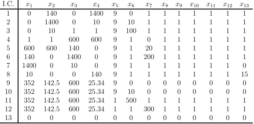
4.5 Varying the initial conditions in the FSH system . . . 54

4.6 Varying the initial conditions in the ovarian system . . . 56

5.1 Varying the Initial Conditions in the Merged System. . . 85

7.1 Description of the Merged System Variables . . . 111

7.2 Description of the Merged System Parameters . . . 112

7.3 Merged System Variable Substitutions . . . 117

7.4 Unit Carrying Constants . . . 122

7.5 Dimensionless Groups of Parameters . . . 125

7.6 Dimensionless Parameter Values . . . 126

A.1 Daily Mean Serum Levels of Estradiol, Progesterone, Inhibin, Lutieniz-ing Hormone, and Follicle StimulatLutieniz-ing Hormone in Normally CyclLutieniz-ing Women (estimated from McLachlanet al. [41]) . . . 144

A.2 Estimates for the Ovarian Input Function Parameters . . . 147

A.3 Estimates for the Pituiary Input Function Parameters . . . 148

(12)

List of Figures

2.1 Hypothalamus - Pituitary - Ovarian Axis . . . 6

2.2 The Phases of the Menstrual Cycle . . . 8

3.1 Ovarian Hormone Data . . . 13

3.2 Pituitary Hormone Data . . . 14

3.3 Ovarian Hormone Input Functions . . . 16

3.4 Stages of Follicular and Luteal Development . . . 24

3.5 Pituitary Hormone Input Functions . . . 25

4.1 Nelder Mead Simplex Choices . . . 42

4.2 Graph of FSH serum concentrations as predicted by the FSH system 45 4.3 Graph of LH serum concentrations as predicted by the LH system . . 46

4.4 Graphs of the ovarian state variables predicted by the ovarian system 50 4.5 Stages of Follicular and Luteal Development . . . 51

4.6 Graph of E₂ serum concentrations as predicted by the ovarian system 52 4.7 Graph of P₄ serum concentrations as predicted by the ovarian system 53 4.8 Graph of Ih serum concentrations as predicted by the ovarian system 53 4.9 Results of varying initial conditions in the pituitary systems . . . 55

4.10 Results of varying initial conditions in the ovarian system . . . 57

5.1 Graph of LH as predicted by the merged system . . . 77

5.2 Graph of FSH as predicted by the merged system . . . 78

5.3 Graphs of the ovarian hormones predicted by the merged system . . . 79

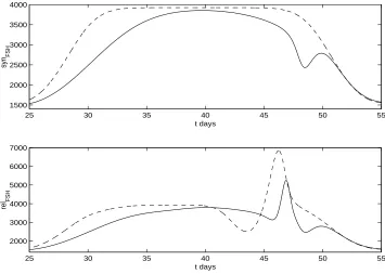
5.4 Comparison ofsynF SH and relF SH in Unmerged and Merged Systems 80 5.5 FSH, LH, and estradiol blood levels as a result of varying initial con-ditions in the merged system . . . 86

5.6 (a) Existence of Hopf bifurcation when varyingn. (b) Branch of stable periodic solutions arising from the bifurcation. . . 91

5.7 Existence of a second Hopf point when varying n. . . . 92

(13)

5.8 (a) Branch of stable periodic solutions arising from the bifurcation. (b) Period along branch of periodic solutions when varyingk₂. . . 93 5.9 Branches of Hopf points in (k₂,dinh), (n, k2) space. . . 95

6.1 LH and FSH blood levels of the two stable periodic solutions as pre-dicted by the merged system. . . 98 6.2 E₂, P₄, and Ih blood levels of the two stable periodic solutions as

predicted by the merged system. . . 99 6.3 Restoring the normal circulation of hormones after 5 day progesterone

treatment. . . 101 6.4 Pituitary hormones after the administration of 80nmol/L of

proges-terone. . . 102 6.5 Ovarian hormones after the administration of 80nmol/Lof progesterone.102 6.6 Pituitary hormones after the administration of 50nmol/L of

proges-terone. . . 103 6.7 Ovarian hormones after the administration of 50nmol/Lof progesterone.103 6.8 Restoring the normal circulation of hormones after 5 day estrogen

treatment. . . 104 6.9 Estradiol levels after 5 and 10 day estrogen treatments (50ng/L). . . 105 6.10 Normal cycle is not recovered after 20 day estrogen treatment. . . 106 6.11 Disruption of the normal cycle by exogenous estrogen leads to

abnor-malities in the menstrual cycle. . . 107 7.1 Graphs of the pituitary hormones as predicted by the dimensionless

merged system. . . 127 7.2 Graphs of the ovarian hormones as predicted by the dimensionless

merged system. . . 128

(14)

Chapter 1 Introduction

Ovarian and pituitary hormones work together to regulate and maintain the men-strual cycle in adult women. The menmen-strual cycle is made up of two phases: the follicular phase and the luteal phase separated by ovulation and menstruation. Dur-ing the menstrual cycle, the pituitary secretes hormones that stimulate the growth and development of ovarian follicles. Consequently, these follicles secrete hormones which control the secretion of pituitary hormones. The pituitary and ovarian hor-mones work together to release an ovum (egg) to be fertilized. If fertilization does not occur, the cycle is repeated. The menstrual cycle is an integral part of the sex-ual endocrine system, therefore many clinical studies have been performed to better understand the mechanisms controlling this process. The behavior of the hormones that control the menstrual cycle can be modeled mathematically using differential equations that describe their interactions throughout the cycle.

In this work a model that predicts the blood concentrations of five hormones pro-duced in the ovary and the pituitary as they interact to regulate and maintain the menstrual cycle will be presented. The model has three components: the pituitary component, the ovarian component, and the merged component. The first two com-ponents of the model were first developed by Schlosser and Selgrade in [50, 54]. The

(15)

Chapter 1. Introduction 2

first component of the model consists of systems of ordinary differential equations that describe the synthesis, release, and clearance of the pituitary hormones, follicle-stimulating hormone (FSH) and luteinizing hormone (LH) during the menstrual cycle, based on their response to the ovarian hormones estradiol (E₂), progesterone (P₄), and inhibin (Ih). Functions representing the ovarian hormones are used as inputs into these systems. The input functions were approximated using data from the lit-erature [41] for the serum levels of E₂, P₄, and Ih during the menstrual cycles of 33 normally cycling women. The second component of the model is a system of ordinary differential equations that describes the roles of FSH and LH in the development of ovarian follicles and the production of the ovarian hormones, E₂, P₄, and Ih, during the menstrual cycle. Functions representing the pituitary hormones are used as inputs into this system. The final component of the model is the merged system formed by merging the pituitary and ovarian components together. This system is a nonlinear system of delay differential equations that describes the interactions between the five hormones throughout the menstrual cycle.

(16)

Therefore a mathematical model that accurately predicts the serum levels of hormones that control the menstrual cycle would be a useful tool in evaluating the effects of exogenous compounds on the sexual endocrine system. In addition, such a model could be used to test the effects of various hormonal methods of birth control such as birth control pills, skin implants, and liquid injectables [33].

A review of various mathematical models of the human menstrual cycle from the literature can be found in [12]. Many of these models are descriptive rather than predictive and do not rely upon physiological mechanisms that control the cycle. In addition, many models only address certain aspects of the menstrual cycle. For ex-ample, models describing the effect of estradiol on serum levels of LH and FSH and vice versa during the menstrual cycle that do not address the effects of progesterone and inhibin [12, 35]. The model to be presented in this work is based on the physi-olgical mechanisms in the hypothalamus, the pituitary, and the ovary that regulate and maintain the menstrual cycle through the synthesis and release of hormones, the development of ovarian follicles, and the positive and negative feedback relationships of hormones during the cycle.

(17)

(18)

Chapter 2 The Biological System

2.1 The Hypothalamus-Pituitary-Ovarian Axis

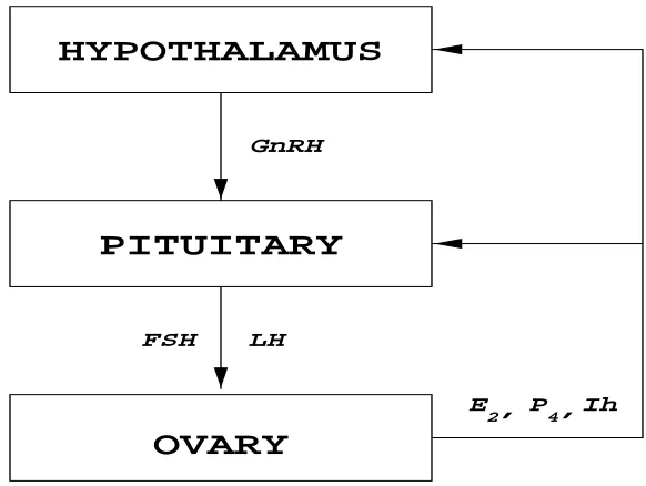
The endocrine system is a communication system of glands that regulate certain body functions through the secretion of hormones into interstitial tissue. Hormones are chemical molecules produced in the cells of endocrine glands which send messages to other cells in target organs [45, 49]. Most hormones are carried to their target organs by the blood, while some hormones act on cells within the organ in which they are produced [49]. The hypothalamus, the pituitary, and the ovary are all en-docrine glands that communicate with each other to regulate a woman’s reproductive system. The hypothalamus is the part of the brain that connects the central ner-vous system to the endocrine system via the Hypothalamus-Pituitary-Ovarian Axis (HPO). By releasing the hormone Gonadotropin-Releasing Hormone (GnRH) into the blood, the hypothalamus signals the anterior lobe of the pituitary gland to produce the hormones, Follicle-Stimulating Hormone (FSH) and Luteinizing Hormone (LH) [34]. FSH and LH are called gonadotropins because they stimulate the gonads, the human reproductive glands.

In women the gonadal gland is the ovary. FSH and LH control the development

(19)

Chapter 2. The Biological System 6

of the ovarian follicles and the corpus lutea, and hence play an important role in the production of ovarian hormones. Through negative and positive feedback loops to the hypothalamus and/or the pituitary, the ovarian hormones regulate the production of LH and FSH [34]. This hormonal control system is illustrated in Figure 2.1. A similar control system exists in men, but will not be discussed in this work.

E _{P ,}

2, 4 Ih

FSH LH GnRH

HYPOTHALAMUS

PITUITARY

OVARY

Figure 2.1: Hypothalamus - Pituitary - Ovarian Axis

(20)

of menopause because some of these follicles are selected to undergo several stages of growth and development, while the rest are left to undergo atresia, a process of degeneration. On average, only about 400 growing follicles will be chosen to ovulate in an woman’s lifetime [49].

2.2 The Menstrual Cycle

Before puberty, the hormonal control mechanism described in the previous section is not functioning. Therefore the production of LH and FSH in the pituitary is “irregu-lar” (non-cyclic) [45]. The beginning of a woman’s reproductive years marks a change in the production of the gonadotropins and a change in the ovaries’ responsiveness to them [49]. At this time, the cyclic process called the menstrual cycle begins. This process is regulated by the secretion of GnRH from the hypothalamus, LH and FSH from the pituitary, and estradiol (E₂), progesterone (P₄), and inhibin (Ih) from the ovary. A normal menstrual cycle lasts for 25-32 days [41] and consists of two phases, the follicular phase and the luteal phase separated by ovulation and menstruation, respectively. A schematic diagram of the menstrual cycle is shown in Figure 2.2.

(21)

Pituitary

growth

follicle

ovulation FSH

FSH

LH LH

E₂

E 2

P₄ P

4 _Ih

E 2 P4 Ih

corpus

luteum corpus

luteum

Hypothalamus menstruation

preovulatory

Figure 2.2: The Phases of the Menstrual Cycle: Appeared in the Fields Institute Communications, Volume 21, 1999, Selgrade and Schlosser.

next cycle [53].

(22)

Before each menstrual cycle, several inactive follicles called primordial follicles are selected to grow into primary follicles. The growth of primordial follicles into primary follicles does not depend on hormonal secretion from the pituitary [49], therefore we will not discuss that process in this work. Primary follicles consist of an egg surrounded by a single layer of granulosa cells, and a basement membrane. The granulosa cells inside the follicles have FSH receptors. Receptors are proteins formed on the membrane of a cell or within the cell which bind to hormones targeting that cell. These receptors are needed for a hormonal stimulus to take effect [45, 61].

(23)

(24)

Chapter 3 The Unmerged Model: Model

Assumptions and Structure

In this chapter we will discuss the mathematical structure of the unmerged model which has two components: the pituitary component and the ovarian component. The pituitary component depicts the ovary’s hormonal control of the pituitary, while the ovarian component depicts the pituitary’s hormonal control of the ovary. The first two components were presented in [50, 54] by Schlosser and Selgrade. The authors focused on the hormonal structure of the HPO axis and the qualitative behavior of the five hormones that regulate the menstrual cycle. In this work we will: (i) optimize the model parameters so that the output yields good approximations to data found in literature, (ii) study the stability of model simulations, and (iii) validate the model by merging the first two components together and testing the effects of external forcing on the output. The merged model will describe the hormonal interaction between the pituitary and the ovary throughout the menstrual cycle. This model will be discussed in detail in Chapter 5.

(25)

Chapter 3. The Unmerged Model: Model Assumptions and Structure 12

3.1 The Pituitary Component

The pituitary component describes the synthesis, release, and clearance of FSH and LH based on the pituitary’s response to serum levels of E₂, P₄, and, Ih.This compo-nent consists of two systems, the FSH system and the LH system, of 2-dimensional ordinary differential equations with time dependent coefficients. Each system is linear in its state variables, however the time dependent coefficients are nonlinear functions of the ovarian hormones. Equations representing the serum levels of the ovarian hormones during a menstrual cycle are used as inputs into the pituitary systems in order to predict the serum levels of the pituitary hormones during that cycle. The input functions are chosen so that they approximate the data for serum levels of E₂, P₄, and Ih found in the McLachlan et al. paper [41] and that the resulting levels of FSH and LH also fit the data in this paper.

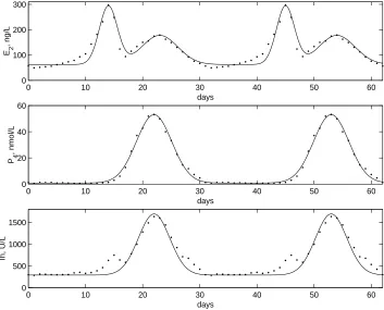
This data was used throughout this modeling process because this was the only paper we could find that presented the full hormone profiles for each of the five hormones we are modeling. The hormone profiles presented in the McLachlan paper are illustrated in Figures 3.1 and 3.2 and the approximate serum levels are listed in Table A.1 in Appendix A. The authors of [41] describe an experiment that was performed on 33 normally cycling women whose hormone levels were recorded each day for a complete cycle. The data values for each woman were then normalized around the day of her LH surge so that the data for all 33 women could be averaged together to get the daily mean serum levels in Table A.1 [41]. This lumped data is used to represent the blood levels of the pituitary and ovarian hormones during a normal menstrual cycle.

(26)

0 5 10 15 20 25 30

0 100 200 300

days

Estradiol, ng/L

0 5 10 15 20 25 30

0 20 40 60

days

Progesterone, nmol/L

0 5 10 15 20 25 30

0 500 1000 1500

days

Inhibin, U/L

Figure 3.1: Daily mean serum levels of estradiol, progesterone, and inhibin of 33 normally cycling women. Appeared in McLachlan et al. [41].

is necessary to assume that the hormone data is periodic. The period is chosen to be p = 31 for the following reasons: (i) the blood concentration of each hormone at day 30 is greater than the level on day 0, and (ii) the slope of the tangent line of the data points at day 30 is negative (ie. the data is decreasing at day 30). Therefore we make the assumption that the hormone levels at day 31 are equal to those at day 0 and that the serum levels repeat every 31 days.

(27)

0 10 20 30 40 50 60

0 100 200 300 400

days

LH,

µ

g/L

0 10 20 30 40 50 60

50 100 150 200 250 300 350

days

FSH,

µ

g/L

Figure 3.2: Daily mean serum levels of FSH and LH of 33 normally cycling women. Appeared in McLachlanet al. [41].

(28)

before midcycle and the other occuring on day 23 during the luteal phase of the cy-cle. Similarly, the input functions for P₄ and Ih over one period contain a constant term and one exponential term characterizing the peak of each of these hormones on day 22 during the luteal phase of the cycle. In order to approximate periodic data, exponential terms are added to the input functions to characterize the peaks for as many periods as we wish to consider. The input functions used to approximate the ovarian hormone data over two periods of data are as follows:

E₂(t) = e₀+e₁e−(t−14)2e₂ ₊_e

3e−

(t−23)2 e₄ ₊_e

1e−

(t−45)2 e₂ ₊_e

3e−

(t−54)2

e₄ _, _(3.1)

P₄(t) = pr₀+pr₁e−(t−22)2pr₂ ₊_pr

1e−

(t−53)2

pr₂ _, _(3.2)

Ih(t) = h₀ +h₁e−(t−22)2h₂ ₊_h

1e−

(t−53)2

h₂ _. _(3.3)

(29)

0 10 20 30 40 50 60

0 100 200 300

days

E 2

, ng/L

0 10 20 30 40 50 60

0 20 40 60

days

P 4

, nmol/L

0 10 20 30 40 50 60

0 500 1000 1500

days

Ih, U/L

Figure 3.3: The ovarian hormone input functions used in the pituitary component of the model as compared to the data in the McLachlan paper.

(30)

In this model, gonadotropin synthesis and gonadotropin release are treated as separate processes [50, 54]. This is an important feature of the model because these processes have different control mechanisms. Synthesis refers to hormone production and the formation of a releasable pool in secretory vesicles [50], while release refers to secretion into the blood. The pituitary secretes FSH and LH into the blood in response to GnRH. However, due to the complex nature of GnRH synthesis and release, this model lumps together the direct regulation of the pituitary and the indirect regulation of the pituitary via GnRH release from the hypothalamus as one control mechanism [50, 54]. Therefore the ovary’s indirect regulation of the pituitary, characterized by the release of GnRH in response to the serum levels of the ovarian hormones, appears implicitly in the FSH and LH release terms of the pituitary systems. FSH and LH are secreted in a pulsatile manner, however, it is assumed that the ovary responds to average blood levels of FSH and LH [43]. Therefore, the systems in the pituitary component predict the average blood concentrations of FSH and LH throughout the menstrual cycle [54].

The FSH system consists of two coupled differential equations, one corresponding to RPF SH in the pituitary and the other corresponding to FSH in the blood. Changes

in RPF SH(t) are determined by the amount of FSH synthesized in the pituitary and

the amount of FSH released into the blood. Similarly, changes in FSH(t) are deter-mined by the amount of FSH released into the blood and the amount cleared from the blood. The synthesis, release, and clearance rates for FSH are denoted by synF SH,

(31)

d

dtRPF SH = synF SH −relF SH (3.4) d

dtF SH = 1 vdis

relF SH−clearF SH (3.5)

The parameter vdis represents the volume of distribution which is the portion of

the blood throughout which hormones are circulated after release. It is this propor-tionality constant which relates the concentration of a hormone in the blood and the amount of that hormone produced in the body by the relation [32, 59]:

Concentration = Amount

Volume of Distribution.

(32)

to be proportional to amount of FSH on reserve in the pituitary, therefore

relF SH =relF SH(E2, P4, RPF SH).

There is evidence that inhibin has an inhibitory effect on FSH synthesis [26, 30, 41, 52]. Therefore the synthesis rate of FSH is assumed to be a function of inhibin concentrations, that is

synF SH =synF SH(Ih).

The period of time between changes in inhibin blood levels and changes in the syn-thesis rates of FSH is captured by incorporating a time delay, δIh, into the input

function Ih(t) [50]. Finally, the clearance rate of FSH is assumed to be proportional to FSH blood levels. Therefore the FSH system is of the form:

d

dtRPF SH = synF SH(Ih)−relF SH(E2, P4, RPF SH) (3.6) d

dtF SH = 1 vdis

relF SH(E2, P4, RPF SH)−clearF SH(F SH) (3.7)

where

synF SH(Ih) =

n

1 + Ih(t−δIh) p

(3.8)

relF SH(E₂, P₄, RPF SH) =

q(1 +rP₄(t))

(33)

clearF SH(F SH) = clF F SH (3.10)

The compartmental structure of the LH system is identical to that of the FSH system with state variables RPLH and LH. However there are variations in the

synthe-sis and release terms because LH responds differently to ovarian hormone secretion. Recall that estradiol and progesterone have a similar effect on LH release as they have on FSH release, with the exception that estradiol has a greater inhibitory effect on FSH release. Therefore a first order inhibitory effect of estradiol on LH release is used instead of the second order effect used in the FSH system.

It has been shown that high blood levels of estradiol promote rapid LH synthesis, therefore the numerator of the LH synthesis term contains a Hill function to reflect estradiol’s stimulatory effect on LH. This effect is most evident in the late follicular phase of the menstrual cycle when large amounts of estradiol are secreted by the pre-ovulatory follicle, inducing the LH surge. The Hill function is a fractional expression of estradiol concentrations of the form:

vE₂(t)h

wh+E₂(t)h, (3.11)

(34)

exogenous estrogens to existing estradiol levels.

In the luteal phase of the cycle estradiol blood levels peak for a second time, however, this peak is not as substantial as the late follicular phase peak. It is believed that at this time progesterone blood levels inhibit LH synthesis [53]. As with Ih(t) in the FSH synthesis term, the time delays δE and δP, are used in the input functions

E₂(t) and P₄(t) which appear in the LH synthesis term. Therefore the LH system has the form:

d

dtRPLH = synLH(E2, P4)−relLH(E2, P4, RPLH) (3.12) d

dtLH = 1 vdis

relLH(E2, P4, RPLH)−clearLH(LH) (3.13)

where

synLH(E2, P4) =

u+ vE2(t−δE)

h

wh+E₂(t−δE)h

1 + P4(t−δP) w₁

, (3.14)

relLH(E2, P4, RPLH) =

y(1 +zP₄(t))

1 +z₁E₂(t) RPLH, (3.15) and

clearLH(LH) = clL LH. (3.16)

(35)

used in the pituitary component of the model and a discussion on how these param-eters can be estimated to fit the data found in the McLachlan paper is provided in Section 4.2.

3.2 The Ovarian Component

The ovarian component of the unmerged model describes the role of the pituitary hor-mones in the development of ovarian follicles and the production of ovarian horhor-mones during the menstrual cycle. Due to the fast time scale of the release and clearance of ovarian hormones [54], the ovarian component is not set up as a two-compartmental model between the ovary and blood as in the pituitary component. Instead, the ovarian component is a 9-dimensional system of ordinary differential equations which track the capacity of the ovary to produce hormones throughout the various stages of the menstrual cycle. The ovary’s capacity at each stage of the cycle is assumed to be proportional to the mass of the follicles or corpus lutea at that stage [54]. In this work we reformulate the ovarian component of the model as presented in [54] to provide a physical meaning to the concept of follicular “capacity”. Here the state variables are chosen to represent the mass of the “active” follicular or luteal tissue during the corresponding stage of the cycle. By “active” mass we mean mass that is growing and secreting hormones.

The ovarian component divides the menstrual cycle into 9 distinct stages of fol-licular and luteal development. The folfol-licular phase of the cycle is divided into three stages:

(36)

ii. Secondary Follicular Stage (SeF), representing the growth of the secondary folli-cles induced by FSH and LH; and

iii. Preovulatory Follicular Stage (PrF), representing the selection and growth of the dominant follicle stimulated by LH.

The period separating the follicular and luteal phases is divided into two stages: i. Ovulatory Scar 1 (Sc₁), representing ovulation; and

ii. Ovulatory Scar 2 (Sc₂), representing luteinization.

The luteal phase is divided into four stages of luteal development:

Luti for i= 1, . . . ,4.

A schematic diagram (adapted from a graph by Dr. Paul Schlosser) outlining the effect of gonadotropin secretion on the nine stages of follicular and luteal develop-ment is shown in Figure 3.4. The ovarian system is linear in its state variables with time dependent coefficients that are nonlinear functions of the pituitary hormones. M sF(t), SeF(t), P rF(t), Sc₁(t), Sc₂(t), Lut₁(t), Lut₂(t), Lut₃(t), and Lut₄(t), are the state variables in this system representing the mass of the follicular and/or luteal secretory tissue which is active during the corresponding stage of the cycle.

(37)

Chapter 3. The Unmerged Model: Model Assumptions and Structure 24 LH LH LH E₂ P₄ Ih FSH MsF Menstrual Follicles Ovulatory Scars Sc1, Sc2 Lut1,Lut2, Lut3, Lut4

Secondary Follicles SeF PrF Preovulatory Follicle Follicles Inactive Corpus Luteum

Figure 3.4: Stages of follicular and luteal development throughout the menstrual cycle.

a good approximation. The input functions we used to approximate two periods of pituitary data are:

F SH(t) = f₁e−(tf−5)2₂ ₊_f

3e

−(t−15)2 f₄ ₊_f

5e

−(t−18)2 f₆ ₊_f

7e

−(t−36)2 f₈

f₉e−(tf−46)2₁₀ ₊_f

5e

−(t−49)2 f₆ ₊_f

7e

−(t−67)2

f₁₁ _, _(3.17)

LH(t) = l₀+l₁e−(tl−7)2₂ ₊_l

3e

−(t−15)2 l₄ ₊_l

5e

−(t−18)2 l₆ ₊_l

1e

−(t−38)2 l₂

+l₃e−(t−46)2l₄ ₊_l

5e

−(t−49)2 l₆ ₊_l

1e

−(t−69)2

(38)

Using the parameters values found in Table A.3, the input functions used in the ovarian system are graphed against the data from the McLachlan paper in Figure 3.5.

0 10 20 30 40 50 60

0 100 200 300 400

days

LH,

µ

g/L

0 10 20 30 40 50 60

50 100 150 200 250 300 350

days

FSH,

µ

g/L

Figure 3.5: The pituitary hormone input functions used in the ovarian component of the model as compared to the data in the McLachlan paper.

Each of the nine variables in the ovarian system is a continuous function of time with the following behavior:

a) it increases as the mass corresponding to that stage of development becomes active, b) it reaches a peak during its highest level of activity, and then

(39)

A transfer of activity occurs from each stage to the next. For example, one follicle is chosen from the growing secondary follicles to be the dominant follicle that continues to grow until it ovulates. This represents a transfer of activity from the Secondary Follicular Stage to the Preovulatory Follicular Stage. Hence, as the SeF(t) is de-creasing because the mass in that stage is becoming inactive, the function PrF(t) is increasing because the mass in that stage is becoming active.

In revising the model in [54], we opted to add an additional parameter to the system equations, LH₀, for dimensional consistency in the case when the exponents of LH are fractions. The parameter LH₀ will have the same units as LH as it will represent a unit of measurement of LH. Therefore the ovarian system has the form:

d

dtM sF = b F SH(t) +

·

c₁F SH(t)−c₂

µ

LH(t) LH₀

¶α¸

M sF (3.19)

d

dtSeF = c2

µ

LH(t) LH₀

¶α

M sF +

" c₃ µ LH(t) LH₀ ¶β

−c₄

µ LH(t) LH₀ ¶# SeF(3.20) d

dtP rF = c4

µ

LH(t) LH₀

¶

SeF −c₅

µ

LH(t) LH₀

¶γ

P rF (3.21)

d

dtSc1 = c5

µ

LH(t) LH₀

¶γ

P rF −d₁Sc₁ (3.22)

d

dtSc2 = d1Sc1−d2Sc2 (3.23)

d

dtLut1 = d2Sc2−k1Lut1 (3.24)

d

dtLut2 = k1Lut1−k2Lut2 (3.25)

d

(40)

of change of each of the ovarian hormone concentrations can be written as:

d C d t =

1 vdis

9

X

i₌₁

siFi(t)−δ C, (3.28)

whereC represents the hormone’s blood concentration, Fi represents the active mass

of follicular or luteal tissue in theith_{stage of the ovarian system,}_s

i represents the

hor-mone’s secretion rate during theith _{stage of the cycle, and}_δ_{represents the hormone’s}

clearance rate. We assume that the clearance of the ovarian hormones from the blood is rapid compared to the development of follicles and corpus lutea (ie. the time scale is much faster) [35] and, hence, δ is large. Dividing through by δ in equation (3.28) yields the left hand side ²dC_dt, where ² = 1_δ. Therefore the system in (3.19)-(3.27), together with the differential equation in (3.28) can be written as:

dF

dt = g(F, t), (3.29)

²dC

dt = h(F, C, t), (3.30)

whereF = (M sF, SeF, P rF, Sc₁, Sc₂, Lut₁, Lut₂, Lut₃, Lut₄) and²is small [2]. Using the “pseudo-steady state” hypothesis [2, 35, 42], we assume that ²dC_dt ≈0 and hence equation (3.28) reduces to:

C(t)≈ 9

X

i=1

CiFi(t), (3.31)

where the coefficientCi = _{δ v}si

dis weights thei

th_{stage’s contribution to the total amount}

of hormone produced throughout the cycle.

(41)

Est(t) may be written as a linear combination of SeF, PrF, and Lut₄, that is:

Est(t) = e₁+e₂SeF(t) +e₃P rF(t) +e₄Lut₄(t). (3.32)

Progesterone and inhibin are secreted mainly in the luteal phase by the corpus lu-teum, however inhibin is also secreted by the preovulatory follicle. Therefore the concentrations of P₄ and Ih denoted by Prog(t) and Inh(t) may be written as:

P rog(t) = pr₁Lut₃(t) +pr₂Lut₄(t),and (3.33)

(42)

Chapter 4 Analyzing the Unmerged Model

The unmerged model consists of three systems of ordinary differential equations, the FSH system, the LH system, and the ovarian system. In order to determine whether these systems accurately predict the blood levels of the pituitary and ovarian hormones during the menstrual cycle, we must first find estimates for the system parameters. In this chapter, we provide theoretical results for the existence and uniqueness of solutions and a description of the parameter optimization techniques used in this project. We also present numerical and stability results obtained from using the parameter values in the pituitary and ovarian systems.

4.1 Theoretical Results for the Pituitary and

Ovar-ian Systems

Each of the pituitary and ovarian systems can be written in the form [54]:

X0 = A(t)X+B(t) (4.1)

(43)

Chapter 4. Analyzing the Unmerged Model 30

where A(t) is a continuous matrix on [0,∞) and B(t) is a continuous vector on [0,∞). The following theorem ensures the existence and uniqueness of a solution to the system in (4.1) with X(0) =X₀.

Theorem 4.1. Existence and Uniqueness of Linear, Non-autonomous

Systems of Ordinary Differential Equations. If A(t) and B(t) are continuous on [0,∞) and ||X₀|| < ∞, then the system in (4.1) has a unique solution X(t) on

[0,∞) that satisfies the initial condition X(0) =X₀ [8].

Using the variations of constants formula [8, 46] for linear, non-autonomous sys-tems of ordinary differential equations, these syssys-tems can be solved explicitly. The closed form solutions for each system will be presented in this section.

The FSH System

If we letX = (X₁, X₂) = (RPF SH, F SH)∈R2, then the FSH system in (3.6)-(3.7)

can be written as:

X0 = AF(t)X+BF(t), (4.2)

where

AF(t) = 

 aF11(t) aF12(t)

aF

21(t) aF22(t)



=

     

− q(1 +rP4(t))

1 +sE₂(t)2 0 q(1 +rP₄(t))

vdis(1 +sE2(t)2) −

clF     

, (4.3)

and

BF(t) = 

 bF1(t)

bF₂(t)



=



 1 +Ih(tn−δIh)/p

0



. (4.4)

(44)

functions E₂(t), P₄(t), and Ih(t) are all continuous. By the variations of constant formula [8, 46], if ΦF(t) is a fundamental matrix of the system,

X0 = AF(t)X, (4.5)

then the solution of (4.2) with the initial condition X(0) =X₀ is given by:

X(t) = ΦF(t) Φ−F1(0) X0+ ΦF(t)

Z t

0

Φ−_F1(τ)BF(τ)dτ. (4.6)

A fundamental matrix of the system in (4.5) is a nonsingular, solution matrix. This system can be rewritten as:

X₁0 = aF₁₁(t)X₁ (4.7)

X₂0 = aF₂₁(t)X₁+aF₂₂(t)X₂. (4.8)

A fundamental matrix, ΦF(t), satisfying ΦF(0) =I, can be found by solving the first

equation and then substituting the result into the second equation and solving. Using the integrating factore−R0taF11(τ)dτ _{the following solution to (4.7) is obtained:}

X₁(t) =X₁(0)eR0taF11(τ)dτ_. _(4.9)

After substituting this equation into (4.8) for X₁(t) we obtain:

X₂0−aF₂₂(t)X₂ =aF₂₁(t)X₁(0) eR0taF11(τ)dτ_. _(4.10)

Multiplying both sides by the integrating factore−R0taF22(τ)dτ _yields:

d dt

³

X₂e−R0taF22(τ)dτ

´

(45)

Integrating both sides of (4.11) from 0 to t we obtain the solution:

X₂(t) = X₂(0)eR0taF22(τ)dτ

+ X₁(0)eR0taF22(τ)dτ

Z t

0

aF₂₁(s)eR0s[aF11(τ)−aF22(τ)]dτ_ds _(4.12)

Therefore the solution matrix of (4.5) with ΦF(0) =I has the form:

ΦF(t) =     

eR0taF11(s)ds ₀

eR0taF22(τ)dτRt

0 aF21(s)e Rs

0[aF11(τ)−aF22(τ)]dτ_ds _eR0taF22(s)ds_.

   

 (4.13)

To check whether ΦF(t) is a fundamental matrix we need to determine thedetΦF(t).

By Abel’s formula [8, 46],

detΦF(t) =detΦF(0)e

Rt

0P2i=1aFii(τ)dτ_. _(4.14)

ThereforedetΦF(t) = e

Rt

0P2i=1aFii(τ)dτ 6= 0 since detΦ_F(0) = det(I) = 1 and ex 6= 0 for

any x. Hence ΦF(t) is a fundamental matrix of (4.5) with ΦF(0) =I.

The LH System

Similarly, if we let Y = (y, Y₂) = (RPLH, LH) ∈ R2, then the LH system in

(3.12)-(3.13) can be written as:

(46)

where

AL(t) = 

 aL11(t) aL12(t)

aL

21(t) aL22(t)

 =      

− y(1 +zP4(t))

1 +z₁E₂(t) 0 y(1 +zP₄(t))

vdis(1 +z1E2(t)) −

clL     

, (4.16)

and

BL(t) =     

bL₁(t)

bL₂(t)

    =        

u+ vE2(t−δE)

h

wh+E₂(t−δE)h

1 +P₄(t−δP)/w1

0         . (4.17)

AL(t) is a continuous matrix and BL(t) is a continuous vector, provided that the

input functions, E₂(t) and P₄(t), are both continuous. Therfore by the variations of constant formula, the solution of (4.15) with the initial condition Y(0) =Y₀ is given by:

Y(t) = ΦL(t) Φ−L1(0) Y0+ ΦL(t)

Z t

0

Φ−_L1(τ)BL(τ)dτ, (4.18)

where

ΦL(t) =     

eR0taL11(s)ds ₀

eR0taL22(τ)dτ Rt

0 aL21(s)e Rs

0[aL11(τ)−aL22(τ)]dτ_ds _eR0taL22(s)ds_.

   

 (4.19)

is a fundamental matrix of the system Y 0 = AL(t)Y with ΦL(0) =I.

The Ovarian System

(47)

obtained using a fundamental matrix in the variation of constants formula in the same way as above. If we let

Z = (M sF, SeF, P rF, Sc₁, Sc₂, Lut₁, Lut₂, Lut₃, Lut₄)∈R9,

then the ovarian system in (3.19)-(3.27) can be written as:

Z0 = AOv(t)Z+BOv(t), (4.20)

where

AOv(t) =                        aOv

11(t) 0 0 0 0 0 0 0 0

aOv

21(t) aOv22(t) 0 0 0 0 0 0 0

0 aOv

32(t) aOv33(t) 0 0 0 0 0 0

0 0 aOv

43(t) aOv44(t) 0 0 0 0 0

0 0 0 aOv

54(t) aOv55(t) 0 0 0 0

0 0 0 0 aOv

65(t) aOv66(t) 0 0 0

0 0 0 0 0 aOv

76(t) aOv77(t) 0 0

0 0 0 0 0 0 aOv

87(t) aOv88(t) 0

0 0 0 0 0 0 0 aOv

98(t) aOv99(t)

(48)

and

BOv(t) =                        bOv 1 (t) bOv 2 (t) bOv 3 (t) bOv 4 (t) bOv 5 (t) bOv 6 (t) bOv 7 (t) bOv 8 (t) bOv 9 (t)                        =                       

b F SH(t) 0 0 0 0 0 0 0 0                        . (4.22)

The matrix AOv(t) can be broken into 4 blocks in the following way:

AOv(t) = 

A1Ov(t) A2Ov(t)

0 A3_Ov(t)



, (4.23)

where

A1_Ov(t) =

        

c₁F SH(t)−c₂

³ LH(t)

LH₀

´α

0 0

c₂

³ LH(t)

LH₀

´α

c₃

³ LH(t)

LH₀

´β

−c₄

³ LH(t)

LH₀ ´

0

0 c₄

³ LH(t)

LH0

´

−c₅

³ LH(t)

LH0

´γ

0 0 c₅

³ LH(t)

LH₀ ´γ          , (4.24)

A2_Ov(t) =

       

0 0 0 0 0 0 0 0 0 0 0 0 0 0 0 0 0 0

−d₁ 0 0 0 0 0

(49)

and

A3_Ov(t) =

          

d₁ −d₂ 0 0 0 0 0 d₂ −k₁ 0 0 0 0 0 k₁ −k₂ 0 0 0 0 0 k₂ −k₃ 0

0 0 0 0 k₃ −k₄

          

. (4.26)

AOv(t) is a continuous matrix and BOv(t) is a continuous vector, provided that

the input functions, F SH(t) and LH(t), are both continuous. Therefore by the variations of constant formula, the solution of (4.20) satisfyingZ(0) = Z₀ is given by:

Z(t) = ΦOv(t) Φ−Ov1(0)Z0+ ΦOv(t)

Z t

0

Φ−_Ov1(τ)BOv(τ)dτ, (4.27)

where ΦOv(t) is a fundamental matrix of the system

Z0 = AOv(t)Z (4.28)

(50)

This system can be rewritten as:

Z₁0 = aOv₁₁(t)Z₁ (4.29)

Z₂0 = aOv₂₁(t)Z₁+aOv₂₂(t)Z₂, (4.30) Z₃0 = aOv₃₂(t)Z₂+aOv₃₃(t)Z₃, (4.31) Z₄0 = aOv₄₃(t)Z₃+aOv₄₄(t)Z₄, (4.32) Z₅0 = aOv₅₄(t)Z₄+aOv₅₅(t)Z₅, (4.33) Z₆0 = aOv₆₅(t)Z₅+aOv₆₆(t)Z₆, (4.34) Z₇0 = aOv₇₆(t)Z₆+aOv₇₇(t)Z₇, (4.35) Z₈0 = aOv₈₇(t)Z₇+aOv₈₈(t)Z₈, (4.36) Z₉0 = aOv₉₈(t)Z₈+aOv₉₉(t)Z₉. (4.37)

To find ΦOv(t) we will solve each of the equations in (4.30)-(4.37) by substituting

the previous equation’s solution and integrating from 0 to t. The integrating factors for the system equations are e−R0taOvii (τ)dτ for i = 1, . . . ,9. Therefore the solution to

the first differential equation in (4.29) is:

Z₁(t) =Z₁(0) eR0taOv11(τ)dτ_. _(4.38)

After substituting (4.38) into (4.30) forZ₁ and solving we obtain:

Z₂(t) = Z₂(0)eR0taOv22(τ)dτ ₊_e

Rt

0aOv22(τ)dτ

Z t

0

aOv₂₁(s)Z₁(s)eR0s−aOv22(τ)dτ_ds _(4.39)

= Z₂(0)eR0taOv22(τ)dτ ₊_Z₁_(0)eR0taOv22(τ)dτ

Z t

0

aOv₂₁(s)eR0s[aOv11(τ)−aOv22(τ)]dτ_ds

(51)

for Zi(t) :

Zi(t) = Zi(0)e

Rt

0aOvii (τ)dτ +e

Rt

0aOvii (τ)dτ

Z t

0

aOv_i,i₋₁(s)Zi−1(s)e

Rs

0 −aOvii (τ)dτds. (4.40)

Due to the large number of nested integrals that appear in the fundamental matrix ΦOv(t) derived from (4.38)-(4.40), we will not present the matrix elements

explic-itly. However, we should note that ΦF(t), ΦL(t), and ΦOv(t) are all lower triangular

matrices with diagonal entries:

φF_ii(t) =e−R0taFii(τ)dτ, φL

ii(t) = e−

Rt

0aLii(τ)dτ, and φOv

ii (t) =e−

Rt

0aOvii (τ)dτ (4.41)

(52)

4.2 Estimating Model Parameters

We wish to determine whether the pituitary and ovarian systems accurately predict data values for the blood concentrations of FSH, LH, E₂, P₄, and Ih during a normal menstrual cycle. To achieve this goal we must find estimates for all of the parame-ters in the model. Some of the parameparame-ters have been found experimentally and are presented in literature, however many of the parameters are unknown. In each of the pituitary systems there are two sets of parameters that need to be estimated, the in-put function parameters and the system parameters. However the ovarian system has an additional set of parameters to be estimated, the auxiliary equation parameters.

In order to find optimal estimates for the unknown model parameters, we need a numerical optimization technique that will identify these values. Each parameter set was optimized using a “least squares” curve fitting technique. The goal of the tech-nique is to find the set of parameters that minimizes a “least squares” cost function. For the pituitary systems, we wish to find the set of parameters that minimizes:

C = 62

X

i=0

|f(ti)−Hi|2, (4.42)

whereHi represents the hormone’s blood level given by the data in McLachlanet al.

[41] at timeti = 0, . . . ,62 days (see Table A.1), f(t) represents the hormone’s

(53)

system parameters, the cost function represents the solution error of the differential equations. In each minimization procedure the data values listed in Table A.1 are repeated over two periods and substituted into (4.42) for Hi, i= 1, . . . ,62.

For the ovarian system, the minimization procedure used to estimate the input function parameters is the same as the procedure described above. The input func-tions for FSH and LH given by (3.17) and (3.18) are substituted into (4.42) for f(t). A problem arises when attempting to estimate the ovarian system parameters be-cause there is no data available corresponding to the mass of “active” follicular tissue throughout the menstrual cycle. Therefore a different cost function must be used to estimate the remaining parameters. The auxiliary equations in (3.32), (3.33), and (3.34) are used to approximate the blood levels of the ovarian hormones during the cycle. Therefore, we must use a cost function that calculates the error obtained from the auxiliary equations, which are linear combinations of the ovarian system state variables. The “least squares” cost function we used superposed the error for all of the ovarian hormones in the following way:

C = 62

X

i₌₀

|Est(ti)−Ei|2+|P rog(ti)−Pi|2+|Inh(ti)−Ii|2, (4.43)

where Est(t), P rog(t), andInh(t) are the auxiliary equations in (3.32)-(3.34) and Ei, Pi, andIi, are the data values for estradiol, progesterone, and inhibin listed in

Table A.1 repeated over two periods.

Algorithms were created in MATLAB, a software by MathWorks Inc., to optimize the unknown parameter sets using the “least squares” fit to the data as described above. A key component of the algorithms is the MATLAB function call,

¯

(54)

which uses the Nelder-Mead Simplex Method to find a local minimizer ¯x of a cost function, costf unc, starting with an initial guess, x₀. The Nelder Mead Simplex Method is called a direct search method because it systematically searches through many points ¯x∈ Rn _{until the minimum of a function}_f_(¯_x)_∈_R_{is found [39, 60]. This}

optimization procedure creates a search pattern by iteratively choosing simplices to test. A simplex is a generalized triangle with (n+ 1) vertices in n−space [39]. The method starts with an initial simplex, orders the points on the simplex by their corresponding function values from smallest to largest, and then replaces the worst point (the point on the simplex with the largest function value) with a new point having a lower function value. The new point is obtained by reflecting, expanding, contracting, and/or shrinking the simplex with respect to the worst point. Once the new point is found, it replaces the old point creating a new simplex. The process is continued iteratively until a minimum is found. An outline of the two variable case will follow.

An initial simplex (triangle) is created with a user-defined guess as one of its vertices. The other vertices are selected in the first step of the optimization procedure [39]. The functionf(x, y) is evaluated at each vertex and the vertices are ordered by their function values, ie. V₁ yields the best or lowest value,V₂ yields the next lowest value, and V₃ yields the worst or largest value [39]. Therefore we have the following relation:

f(V₁)≤f(V₂)≤f(V₃). (4.44) A diagram illustrating the choices for the next simplex is shown in Figure 4.1. The steps for creating the new simplex from the initial simplex are as follows [39, 60]:

(55)

●

● ●

V1

R

M C1

C2

● ● ●

●

V2

E V3

●

S

●

Figure 4.1: These are the choices of the next simplex outlined in Steps 1 and 2.

(a) If f(V₁) ≤ f(R) < f(V₂) then replace the worst point V₃ with R forming the new triangleV₁V₂R.

(b) Else if f(R)< f(V₁), then expand R to E.

i. If f(E)< f(R), then replace V₃ withE instead of R forming the new triangle V₁V₂E.

ii. Else if f(E)≥f(R), then form the new triangle with R, V₁V₂R. (c) Otherwise, f(R)≥f(V₂).Go to Step 2: Contract.

2. Contract. Iff(R)≥f(V₂),then contract between the midpointM ofV₁V₂ and the worst point V₃ and the reflection point R, whichever one yields a smaller function value.

(a) If f(V₂) ≤ f(R) < f(V₃), then contract outside to C₁, the midpoint of M R.

(56)

V₁V₂C₁.

ii. Else if f(C₁)> f(R), go to Step 3: Shrink.

(b) Else if f(V₃)≤f(R), then contract inside to C₂, the midpoint of M V₃. i. If f(C₂) ≤ f(V₃), then replace V₃ with C₂ forming the new triangle

V₁V₂C₂.

ii. Else if f(C₂)> f(V₃), go to Step 3: Shrink.

3. Shrink. Iff(C₁)> f(R),orf(C₂)> f(V₃), then shrink the triangleV₁V₂V₃ to V₁M S whereM is the midpoint of V₁V₂ andS is the midpoint ofV₁V₃.The new simplex is V₁M S. Evaluate f at each vertex and order the vertices, renaming them. Then repeat Step 1.

Pituitary System Parameters

Three parameters used in the pituitary systems were not estimated using the optimization procedure described above. The volume of distribution in (3.7) and (3.13) is estimated to bevdis= 2.5Lbecause the average woman has 4−5Lof blood,

55% of which consists of blood plasma and the other 45% consisting of blood cells. Therefore the volume of distribution is approximately 2.5L. [32, 59]. Estimates for the clearance rates for FSH and LH, clF and clL, were derived from measurements

presented in Coble et al. [13] and Kohler et al. [47]. These authors measured the metabolic clearance rates for FSH and LH of pre-menopausal women, ages 20-27, and obtained their average metabolic clearance rates: M CRF SH = 14.2±1.1mL/minand

M CRLH = 24.4±1.8mL/min.To obtain values forclF andclL, we scaled M CRF SH

and M CRLH by the volume of distribution and converted to a time scale of days.

Therefore,

clF =M CRF SH×

1 vdis ×

1440 min

1 day ≈8.2 day