Box-jenkins and genetic algorithm hybrid model for electricity forecasting system

BOX-JENKINS AND GENETIC ALGORITHM HYBRID MODEL FOR ELECTRICITY FORECASTING SYSTEM

KHAIRIL ASMANI B. MAHPOL

BOX-JENKINS AND GENETIC ALGORITHM HYBRID MODEL FOR ELECTRICITY FORECASTING SYSTEM

KHAIRIL ASMANI B. MAHPOL

A thesis submitted in fulfilment of the requirements for the award of the degree of

Master of Science (Mathematics)

Faculty of Science Universiti Teknologi Malaysia

To my beloved mum, Asiah bt. Yin, my father, Mahpol Hj. Tahir

ACKNOWLEDGEMENT

Alhamdulillah, by the grace of ALlah S.W.T and the Prophet Muhammad S.A.W, this research is finally completed. It is my greatest pleasure to take this opportunity to express my gratitude and thank you to all the people involved either direct or indirectly in my effort to successfully finish this project.

A deepest gratitude to my supervisor, Assoc. Prof. Dr. Hj. Zuhaimy Hj. Ismail who conducting and advising me on the excel of this research, my beloved parent, brothers and sister who support me and also to all my friends, thank you for your helps and advices that motivate me in completing this master degree. I also indepted to Universiti Teknologi Malaysia (UTM) and Ministry of Science, Technology and Environment for funding my study under UTM-PTP and IRPA Grant Vot. 74047.

To ensure this research follow the standard of academic, I have made thorough reference to books and papers that are relevant to the research title and depth fitering on any sources obtained through mass and electronic media.

ABSTRACT

ABSTRAK

TABLE OF CONTENTS

CHAPTER _TITLE PAGE

TITLE

i

DECLARATION ii

DEDICATION iii

ACKNOWLEDGEMENTS iv

ABSTRACT v

ABSTRAK vi

TABLE OF CONTENTS vii

LIST OF TABLES xiii

LIST OF FIGURES xiv

LIST OF SYMBOLS xvii

LIST OF APPENDICES xx

LIST OF PUBLICATIONS xxi

1 INTRODUCTION 1

1.0 Introduction

1

1.1 Introduction to Forecasting 1

1.2 Problem Background 3

1.3 Problem Statement 5

1.5 Research Importance 7

1.6 Research Scope 7

1.7 Research Data 8

1.8 Research Contribution 8 1.9 Thesis Organization 9

2 LITERATURE REVIEW

11

2.0 Introduction 11

2.1 Energy Demand and Forecasting 11 2.2 Time Series Forecasting Model 13

2.2.1 Moving Average 15

2.2.2 Exponential Smoothing 16 2.2.3 Regression Analysis 18 2.2.4 Box-Jenkins Methodology for

ARIMA Model

20

2.3 Components of Time Series 22 2.4 Forecasting Accuracy 25 2.5 Choosing a Forecasting Technique 26 2.6 Genetic Algorithm (GA) 29 2.7 The Objective and Fitness Function 33

2.8 Population Size 34

2.9 Encoding of a Chromosome 34

2.9.1 Binary Encoding

35

2.9.2 Integer Encoding

35

2.9.3 Real Encoding

2.10 Genetic Algorithm Reproduction Operators 36 2.10.1 Crossover Operator 37 2.10.1.1 Single-Point Crossover 37 2.10.1.2 Multi-Point Crossover 38 2.10.1.3 Uniform Crossover 39 2.10.1.4 Arithmetic Crossover 41 2.10.2 Mutation Operator 41 2.11 Selection Method 43

2.11.1 Roulette Wheel Selection

44

2.11.2 Rank-based Selection

45

2.11.3 Tournament

47

2.11.4 Elitism

47

2.12 Termination of the GA

48

2.12.1 Evolution Time

48

2.12.2 Fitness Threshold

49

2.12.3 Fitness Convergence

49

2.12.4 Population Convergence

49

2.12.5 Gene Convergence

50

2.13 Advantages of Genetic Algorithm 50

2.14 Summary 51

3 RESEARCH METHODOLOGY

3.0 Introduction 52

3.1 Research Approach 52

3.2 Time Series Modeling 53

3.3 ARIMA Models

53

3.3.1 Data Transformation 56 3.3.2 Series with Trend 58 3.3.3 Series with Seasonal Effect 59

3.3.4 Stationarity

60

3.3.5 Autocorrelation Function (ACF)

62

3.3.6 Partial Autocorrelation Function (PACF)

64

3.3.7 Interpreting the Correlogram

65

3.3.8 White Noise

68

3.3.9 Autoregressive Processes

69

3.3.10 Moving Average Processes

69

3.3.11 Mixed Processes

70

3.3.12 Integrated Processes

71

3.3.13 Seasonal ARIMA Modeling

72

3.3.14 Model Identification

73

3.3.15 Conventional Parameter Estimation

76

3.3.16 Forecasting

77

3.4 Parameter Estimation using Genetic Algorithm

78

3.4.4 Reproduction Operator 83

3.4.4.1 Method for Crossover

84

3.4.4.2 Method for Mutation

84

3.4.5 Method for Selection Operator

85

3.4.5.1 Roulette Wheel Technique

86

3.4.5.2 Elitism Operator

87

3.4.6 Termination Criteria

88

3.5 Computer Simulation 88

3.6 Summary 90

4 FORECAST OF MALAYSIAN

ELECTRICITY GENERATED

91

4.0 Introduction

91

4.1 The Data 91

4.2 Building Time Series Model 93 4.2.1 Identification Process 93 4.2.2 The Transformation 99 4.2.3 ACF and PACF Plot 101

4.2.4 The Correlogram Analysis

102

4.2.5 ARIMA Forecast with Grid Search

104

4.2.6 Hybrid of ARIMA and Genetic Algorithm Forecast

4.2.7 The Genetic Algorithm (GA)

Calculation

110

4.2.7.1 Production of Initial Population

112

4.2.7.2 Fitness Function Calculation

113

4.2.7.3 Selection Calculation

116

4.2.7.4 Uniform Crossover and Mutation Calculation

118

4.3 Summary

120

5 DEVELOPMENT OF INTELLIGENT

ELECTRICITY FORECASTING SYSTEM (IEFS)

121

5.0 Introduction 121

5.1 Our Model: IEFS 121

5.2 System Approaches and Methodology

123

5.2.1 Prototype Methodology 125 5.2.2 System Design 125 5.2.2.1 Users and Their

Characteristics

126

5.2.2.2 Identify User Task

126

5.2.2.3 Continuous User

Involvement

5.3 System Implementation 127

5.3.1 Main Window 127

5.3.2 Database Window 129 5.3.3 GA Properties and Estimation

Window

130

5.3.4 Forecast Result and Graph Window 132 5.4 Data Structure and Resourced Used 134 5.5 System Schedule 135

5.5 Summary

136

6 CONCLUSION AND

RECOMMENDATIONS FOR FURTHER RESEARCH

137

6.0 Introduction 137

6.1 Results and Discussion 137

6.1.1 Malaysian Electricity Generated Data Analysis

138

6.2 Conclusion 141

6.3 Recommendations for Future Work

142

REFERENCES

145

APPENDICES A – H

LIST OF TABLES

TABLE NO. _TITLE

PAGE

2.1 Advantages of Using Genetic Algorithm 51

3.1 Specific Box-Jenkins Models 67 3.2 Roulette Wheel Probability Calculation 86

4.1 Monthly Electricity Generated (kWh) at Power Plants 93 4.2 Trend and Cyclical-Seasonal Irregular Analysis 96 4.3 Transformation, Ln

( )

4.4 Model Identification using Try and Error Approach 105 4.5 Forecast and MSE Fitness for Chromosome

(

)

112

4.6 10 Initial GA Chromosomes 113 4.7 MSE for First Ten GA Populations Simulation 116 4.8 A Sample of GA Search Result 116 4.9 Uniform Crossover Operation 119

4.10 Mutation Calculation 119

4.11 Performance Between Grid Search Versus GA 120 6.1 Forecast Performance Between ARIMA and SARIMA

Models

138

6.2 Forecast Performance Generated by Addictive-Winters and Holt-Addictive-Winters

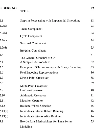
LIST OF FIGURES

FIGURE NO.

TITLE

PAGE

2.1 Steps in Forecasting with Exponential Smoothing 18 2.2(a) Trend Component 23 2.2(b) Cycle Component 24 2.2(c) Seasonal Component 24 2.2(d) Irregular Component 25 2.3

The General Structure of GA

31

2.4 A Simple GA Procedure 32 2.5 Examples of Chromosomes with Binary Encoding 35 2.6 Real Encoding Representations 36

2.7 Single-Point Crossover 38 2.8

Multi-Point Crossover

39

2.9 Uniform Crossover 40

2.10 Arithmetic Crossover 41

2.11 Mutation Operator 42

2.12 Roulette Wheel Selection 45 2.13(a) Individuals Fitness Before Ranking 46 2.13(b) Individuals Fitness After Ranking 46 3.1 Box-Jenkins Methodology for Time Series

Modeling

3.2 Addictive Seasonal Patterns 56

3.3 Multiplicative Seasonal Patterns 57

3.4 Theoretical for ACF 63

3.5 A Non-Stationary ACF Correlogram 67 3.6 A Stationary ACF Correlogram 68 3.7 Model Identification Phase 75 3.8 De-Garis Experiment on Population Sizes Impact 79 3.9 Converting to Binary Encoding 82

3.10 Standard Number Convention for d and b 82 3.11 Binary Based Representation 82

3.12 Flip-Bit Mutation 85

3.13 GA Flowchart for SARIMA Estimation 89 4.1 Malaysian Electricity Generated at Power Plant

(kWh Unit)

95

4.2(a) A Cyclical-Irregular Component 98 4.2(b) A Seasonal-Irregular Component 98 4.3 Transformation,Ln

( )

Process

99

4.4(a) ACF and PACF Correlogram for zt without ∇1 101

4.4(b) ACF and PACF Correlogram for z_t after ∇₁ 102

4.5 A Stationary z_t Values after Differencing of

Order-1, ∇1

103

4.6 A Stationary Residuals Series Generated by the White Noise

103

4.7 Forecast Graph Produce by Various Models using Statistica 5.5

106

4.7(a) SARIMA

(

)(

)

4.7(b) SARIMA

(

)(

)

4.7(d) MA

( )

4.7(e) ARMA

( )

4.7(f) ARIMA

(

)

4.8 Forecast Graph Produce by SARIMA

(

)(

)

using GA

109

5.1 IEFS – Main Window 128 5.2 IEFS – Database Window 129 5.3 IEFS – GA Properties Window 130 5.4 IEFS – GA Estimation Window 132 5.5 IEFS – Forecast Graph Window 133 5.6 IEFS – Forecast Result Window 133 6.1 Addictive-Winters Forecast 139

LIST OF SYMBOLS

GA - Genetic Algorithm

EP - Evolutionary Programming ESs - Evolution Strategies

GUI - Graphical User Interface MSE - Mean Square Error

MAPE - Mean Absolute Percentage Error MAD - Mean Absolute Deviation

SSE - Sum Square Error RMSE - Root Mean Square Error SE - Standard Error AR - Autoregressive MA - Moving Average

I - Integrated

IMA - Integrated Moving Average ARMA - Autoregressive Moving Average ARIMA - Autoregressive Integrated Moving Average SMA - Seasonal Moving Average

SAR - Seasonal Autoregressive

SARIMA - Seasonal Autoregressive Integrated Moving Average MLE - Maximum Likelihood Estimation

LSE - Least Square Estimation TNB - Tenaga Nasional Berhad PTM - Pusat Tenaga Malaysia

RW - Roulette Wheel

SC - Selected Chromosome C/M - Crossover or Mutation Probability Rate kWh - Kilowatt Hour Unit

fc - Final Electricity Consumption

ct - Consumption of Energy Transformed

dl - Losses of Electrical Energy

IEFS - Intelligent Electricity Forecasting System STF - Short Term Forecast

IPP - Independent Power Producer IRP - Integrated Resource Planning ACF - Autocorrelation Function PACF - Partial Autocorrelation Function WAGs - Wild-Assed Guesses

I

C. - Cyclical Irregular Component

I

S. - Seasonal Index

C

T. - Trend Component TSP - Traveling Salesman Problem

SSR - Stochastic Sampling with Replacement IDEs - Integrated Development Environments APIs - Applications Programming Interfaces MB - Mega Byte

GB - Giga Byte

PC - Personal Computer GHz - Giga Hertz

RAM - Read Access Memory NTFS - Network File System

SQL - Structured Query Language O/S - Operating System

t

a , εt - A Series of Shocks Generated by a White Noise

Ln - Natural Logarithm

f d

p. . - Probability Density Function

Cov - Covariance

k

ρ , r_k - Autocorrelation at lag-k

kk

φ - Partial Autocorrelation Function

t

A - Overall Smoothed Estimate

t

B - Trend Estimate

t

Sn - Seasonal Index Estimate

µ _{- Mean}

t - Period of t

LIST OF APPENDICES

APPENDIX NO. _TITLE

PAGE

A Table 4.2 Trend and Cyclical-Seasonal Irregular Analysis 149 B Table 4.3 Transformation, Ln

( )

Process

1

∇ 152

C Table 4.5 Forecast and MSE Fitness for Chromosome, (φ = -0.55, Φ = 0.81, Θ = -0.35)

155

D Table 4.7 MSE for 100 GA Simulation 158 E Table 4.8 GA Search Result 161

F Prototype Methodology 163

G IEFS – System Development Schedule 165

LIST OF PUBLICATIONS

NO.

TITLE

1 Zuhaimy Ismail & Khairil Asmani Mahpol (2005), Emulation of Biological Reproduction System on Forecasting Model, International Symposium on Bio-Inspired Computing, SCRG FSKSM, September 7-9, 2005, Puteri Pan-Pacific Johor Bahru.

2 Zuhaimy Ismail & Khairil Asmani Mahpol (2005), An Intelligent Electricity Forecasting System (IEFS), Laporan Teknik FSUTM, LT/M Bil. 5/2005 3 Zuhaimy Ismail & Khairil Asmani Mahpol (2005), SARIMAT Model for

Forecasting Malaysian Electricity Generated, Jurnal Matematika, UTM : UTM.26/18.11/1/21 Jld.8 (66).

4 Zuhaimy Ismail, Mohd Fuad Jamaluddin and Khairil Asmani Mahpol (2004),

Forecasting of Electricity Demand using ARIMA Models, Proceeding of The Conference Focus Group, RMC UTM, Pulai Spring Golf Resort, Johor Bahru.

5 Zuhaimy Ismail, Khairil Asmani Mahpol & Mohd Fuad Jamaluddin (2004),

Fitting SARIMAT Model for Forecasting Malaysian Electricity Generated, Laporan Teknik FSUTM, LT/M Bil. 5/2004.

6 Zuhaimy Ismail, Mohd Fuad Jamaluddin & Khairil Asmani Mahpol (2003),

Forecast of Energy Generated Using GA – A University-Industry

Collaborative Research, Proceeding of The Conference UNIPRENEUR2003, MARA, 11-12 June, 2003 Renaissance, Kuala Lumpur.

CHAPTER 1

INTRODUCTION

This chapter introduces the reader to the author’s research project. It explains the problem background and description, research objective, research scope, research

importance, research data, research contribution and the significance of this project. It then gives a brief description of the structure of the thesis organization.

1.1 Introduction to Forecasting

Forecasting is defined as an attempt to predict future events. It is also described as a concern of what the future will look like, that act as an aid for effective and efficient planning.

There are two categories of forecasting namely qualitative and quantitative. Qualitative forecasting is a very useful technique when there are no historical data. This method usually uses the opinions of experts to predict the future events subjectively via their experiences and knowledge. The most popular qualitative techniques are the Delphi method, subjective curve fittings and time independent technological comparison.

Quantitative forecasting is a technique that can be applied when there are enough historical data to be modeled in making prediction. This technique involves a depth analysis of the historical data in developing a model. There are two types of quantitative techniques that are univariate and explanatory model. The common time series analysis is normally categorized into both of these types that will be described in details in our literature review.

Forecasting is a very important tool applied in a lot of sectors such as energy consumption, demand and supply, economy, business, sales and market analysis, weather forecast, engineering research and development, science and technology, management and development, industrial, politic and many more. It is very useful because domain experts often have knowledge of events whose effects have not been observed yet in a time series.

In the early 1970s, John Holland has introduced the concept of simulating the process of natural evolution known as GA in computer. Holland’s GA was represented by a sequence of procedural steps for moving from one population of artificial

chromosomes to a new population. It uses natural selection and genetic inspired

techniques known as crossover and mutation. Each chromosome consists of a number of genes that each gene is represented by binary digit of 0 and 1.

GA has received considerable attention regarding its potential as an optimization technique for solving complex problems. It has been successfully applied in the area of industrial engineering that includes scheduling and sequencing, optimization, reliability design, vehicle routing, inventory control, transportation and many more. In this research, the researcher introduces GA as an approach for estimating the parameters in Box-Jenkins method of forecasting.

1.2 Problem Background

Box-Jenkins approach was developed in the 1960s for handling most time series of data analysis. This approach is about to match one Autoregressive Integrated Moving Average (ARIMA) model based on the historical data that currently available in making forecast. Box and Jenkins (1970) effectively put together in a comprehensive manner of the relevant informations required to understand and use univariate time series ARIMA models.

model known as integrated (I) processes will be performed to produce an ARIMA model. If there is seasonality in the data, the models then become either Seasonal Autoregressive (SAR) or Seasonal Moving Average (SMA) or Seasonal Autoregressive Integrated Moving Average (SARIMA). Therefore the general Box-Jenkins model that allows seasonality is:

( )

( )

( )

( )

T Q q i D T d T P

p B Φ B ∇ ∇ z =θ B Θ B a

φ ~ _(1.1)

and is referred to as the multiplicative

(

) (

)

p

φ = unknown pth AR parameter,

q

θ = unknown qth MA parameter,

Φ_P = unknown Pth SAR parameter, ΘQ = unknown Q

th

SMA parameter,

zi = time series value at time i,

a_i = error term at time i,

B = backshift operator, ∇ = difference operator.

The value of the coefficient φ_p,θ_q,Φ_P and Θ_Q are restricted to lie between –1

and +1. Note the minus and plus sign on model is a convention for ARIMA models. The error, a_i, is normally distributed with a mean of 0 and variance of 1.

maximize this function. Then we use the Newton-Raphson numerical optimization to calculate the log likelihood function that is often known as the grid search method.

Many researchers have made comparative studies between GA and other searching techniques, such as random search, grid search, iterated search and simulated annealing. For example, grid search can be a very good method when there is a single unknown parameter to estimate. However, it quickly becomes intractable when the number of elements of θ becomes large.

Grid search method is generally referred to as hill - climbing. They can perform well on functions with only one peak. But on functions with many peaks, they suffered from the problem that the first peak found will be climbed, and this may not be the highest peak. Having reached the top of a local maximum, no further progress can be made (Beasley et. al, 1993). Usually global optimum can be found only if the problem possesses certain convexity properties that essentially guarantee that any local optimum is a global optimum.

1.3 Problem Statement

As describe in the previous section, after we have identified the appropriate ARIMA model, we proceed to estimate its parameters;

( ) (

)

(1.3)

( )

_∑

S

1 2 ,θ α φ

Where the are the estimated shocks given the model and the series.

As described in problem background, it is normal to use a non-linear least squares procedure or MLE to obtain the vector of parameter estimates within the stationary invertible region.

( ) ( )

i θ B φ B z

α = −1

According to Box and Jenkins (1970) the parameters value for ARIMA models are represented by the unknown φ_p,θ_q,Φ_P and Θ_Q where their values are restricted to

lie between –1 and +1. In producing a forecast with the lowest possible error, we need to search the value for these unknown parameters which minimizes the Mean Square Error (MSE). Therefore the main aim of this research are;

1. To study the efficiency of using Genetic Algorithm (GA) to estimate the

parameters φ_p,θ_q,Φ_P and Θ_Q in SARIMA models.

2. To develop an improved method based on GA for univariate forecasting model.

The ergodicity of evolution operators makes genetic algorithm very effective in performing the global search (Mitsuo and Cheng, 1997). This research proposes an alternative approach to the conventional searching method. One such method is the GA which have a potential in giving the optimize value for weighing φ_p,θ_q,Φ_P and thus

improve the forecast result.

Q

1.4 Research Objectives

The main aim of this study is centers around a few fundamental questions such as “What is the role of forecasting process been developed for predicting electricity

generated? Would improve methods give any advantages over current practices? And how statistical method can be integrated to lead to substantial gains in accuracy?”

1.5 Research Importance

This research is highly significant for improving forecast accuracy.

Implementation of GA heuristic search in estimating the parameters in SARIMA model is the major contribution in this study. This work also may improve the univariate Box-Jenkins forecasting model using GA, which may lead in producing a new forecast method using genetic approach.

1.6 Research Scope

1. This research focuses only on the univariate model where the time series based on the past value.

2. Forecast accuracy will be defined by measure the lowest error in term of MSE.

3. In Genetic Algorithm architecture, chromosomes are randomly generated using crossover and mutation operator.

1.7 Research Data

The applications chosen for this study is forecasting the amount of Malaysian electricity generated at power plant. Data used here were a secondary data collected from 1996 to 2003, which has been classified into the total monthly electricity generated in kilowatt hour, kWh unit proposed by Tenaga Nasional Berhad (TNB) as the standard format unit recommended in the energy sectors. The flow of electricity represented by the following equations:

Electricity Generated = fc + ct + dl

= Gross Inland Consumption

Where (fc) is the final electricity consumption refers to the total quantity of electricity delivered to the end-user. The (ct) is the consumption of energy transformed while (dl) refers to losses of electrical energy, which occur outside the utilities and power plants, and the consumption of electricity by utilities and power plants for operating their installation.

1.8 Research Contribution

The main contribution in the research is the development of an algorithm to

search for the best value of φp,θq,ΦP and ΘQ in SARIMA model to minimize the MSE

in making a forecast based on the GA.

1.9 Thesis Organization

This thesis contains six chapters. The first chapter will introduce the problem background and description, research objective, research scope, research importance, research data, research contribution and the significance of this project.

The next chapter is a literature review. In this chapter it contains a discussion on the forecasting using time series method and GA. This chapter will describe the review of the literatures that are related to the past and present study on the electricity generated for Malaysia, time series forecasting and GA procedures, models and applications. It begins by reviewing literature related to time series forecasting model especially Box-Jenkins methodology for ARIMA models. Some comparison study on how selecting the appropriate time series model also discusses in this chapter. After that, researcher made some literature on the problem of searching the SARIMA parameters. Finally, a review of literatures related to GA procedures and application in solving complex searching problem is presented. In GA section, it contains an

introduction to GA, a comparison study done by other researcher on GA with other searching technique, the GA operators, encoding and decoding of a chromosome, selection and the advantages of GA.

The research methodology is described in chapter three. This chapter involved reviewing the existing literature to develop a theoretical framework to form a structure for this research. The chapter begins with describing the theory of time series analysis and the Box-Jenkins methodology for ARIMA model. It then discusses the theory of GA and how it can be applied into Box-Jenkins forecasting.

Chapter four contains the implementation of forecast method at case study. Here, all the sample data of TNB for Malaysian electricity generated is analyzed and used to calculate the forecast step-by-step. All the calculations using hybrid of Box-Jenkins methodology and GA is described in detail in this chapter.

Chapter five discusses on the system develop by the researcher. Intelligence Electricity Forecasting System (IEFS) was developed to realize this research output as an effective decision tool program into computer.

Chapter six presented the results, discussions, conclusions and recommendations for further research. It gives a summary of this research and then discusses in further detail some of results and findings. Some conclusions are drawn and finally, some thoughts on possible directions in which future research in this area might be pursued are offered.