Jurnal Teknologi, 42(D) Jun. 2005: 9–22 © Universiti Teknologi Malaysia
1,2&4
Department of Control and Instrumentation Engineering, Faculty of Electrical Engineering, Universiti Teknologi Malaysia, 81310 Skudai, Johor Bahru, Malaysia.
3
Pusat Pengajian Diploma, Universiti Teknologi Malaysia, Jalan Semarak 54100, Kuala Lumpur.
MODELLING OF PT326 HOT AIR BLOWER TRAINER KIT USING PRBS SIGNAL AND CROSS-CORRELATION TECHNIQUE
MOHD. FUA’AD RAHMAT1, YEOH KEAT HOE2, SAHNIUS USMAN3 & NORHALIZA ABDUL WAHAB4
Abstract. System identification is an experimental approach to determine the transfer function or equivalent mathematical description for the dynamic of a system component by using a suitable input signal. A pseudorandom binary sequence (PRBS) signal of 5 different maximum lengths sequence of 15, 31, 63, 127, and 255 has been used as an input signal to determine the open-loop and closed-loop model of a hot air blower system. The autocorrelation of the input signal and cross-correlation between the input and output signal is performed using the Dynamic Signal Analyzer (DSA) and MATLAB software. From the correlograms of cross-correlation and autocorrelation, the transfer function model can be determined.
Keywords: System identification, pseudorandom binary sequence, autocorrelation, cross-correlation, model validation
Abstrak. Pengenalpastian sistem merupakan suatu ujikaji untuk menentukan rangkap pindah atau matematik model bagi sesuatu sistem dengan menggunakan isyarat masukan yang sesuai. Dalam kertas kerja penyelidikan ini, pseudorandom binary sequence (PRBS) bagi 5 jujukan maksimum yang berlainan iaitu 15, 31, 63, 127, dan 255 digunakan sebagai isyarat masukan untuk menentukan rangkap pindah sistem bagi keadaan gelung buka dan gelung tutup. Fungsi sekaitan auto bagi isyarat masukan dan sekaitan silang bagi isyarat masukan dan keluaran dilaksanakan dengan menggunakan
Dynamic Signal Analyzer (DSA) dan perisian MATLAB. Rangkap pindah kemudiannya ditentukan dari graf sekaitan silang melawan masa lengah dan graf sekaitan auto melawan masa lengah.
Kata kunci: Pengenalpastian sistem, pseudorandom binary sequence, sekaitan auto, sekaitan silang, pengesahan model
1.0 INTRODUCTION
to a set of known inputs, and its outputs are measured. Then, a mathematical model is derived based on the input and output data [1].
There are several reasons for using experimental data to obtain a model of the dynamic system. First, even the best theoretical model built from equations of motion is still only an approximation of reality. Secondly, due to situations where the theoretical model is more complicated, or the physics of the process is poorly understood, the only reliable information is experimental data [2]. The last reason for using experimental data is because the environment of the system sometimes change due to on-line changes that will affect the whole system.
1.1 Pseudorandom Binary Sequence (PRBS)
A pseudorandom binary sequence (PRBS) is a deterministic and periodic sequence of length N that switches between two levels, say +a to another level, say –a [3]. PRBS is a very useful approximation to periodic white noise and it is widely used as forcing functions in statistically system testing. PRBS state can change only at discrete intervals of time, ∆t which is also known as bit interval. State change occurs in a deterministic pseudo random manner. PRBS sequence is periodic with period, T=N∆t where N=integer.
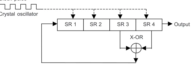
Pseudorandom binary sequence can be generated by means of a serial-input shift register with feedback using exclusive-OR gate as shown in Figure 1. The signal is not truly random because the sequence repeats itself every 2n-1 bit intervals for an n-bit shift register [4].
Figure 1 Block diagram for generation of a MLBS with a shift register (SR) Clock pulse
Crystal oscillator
SR 1 SR 2 Output
X-OR SR 4 SR 3
1.2 Autocorrelation (ACF) and Cross-correlation (CCF)
The process of autocorrelation establishes the relationship between the signal and a time-shifted version of itself. This relationship for all possible time shifts is described by the autocorrelation function. The autocorrelation function (ACF) of a signal x(t) is given the symbol φxx(t) and is defined by Equation (1).
( ) T ( ) ( )
xx
T
T
x t x t dt
T
φ τ + τ
→∞ −
= lim 1
∫
+2
or (1)
( ) T ( ) ( )
xx
T
T
x t x t dt
T
φ τ + τ
→∞ −
= lim 1
∫
−2
A cross-correlation function (CCF) is a process of comparing one signal with another by multiplication of corresponding instantaneous values and taking the average. CCF is also a measure of the similarity between two different signals.
The cross-correlation function of a signal x(t) and y(t) is given the symbol φxy(τ) and is defined as:
( ) lim 1 ( ) ( )
2 T
xy
T
T
x t y t dt
T
φ τ + τ
→∞ −
=
∫
+or (2)
( ) T ( ) ( )
yx
T
T
y t x t dt
T
φ τ + τ
→∞ −
= lim 1
∫
+2
In system identification, x(t) and y(t) are the input and output signal of system being identified.
Table 1 Table for correct stages for n stage shift register
n N Feedback
4 15 3⊕4
5 31 3⊕5
6 63 5⊕6
7 127 4⊕7
1.3 PT326 Process Trainer
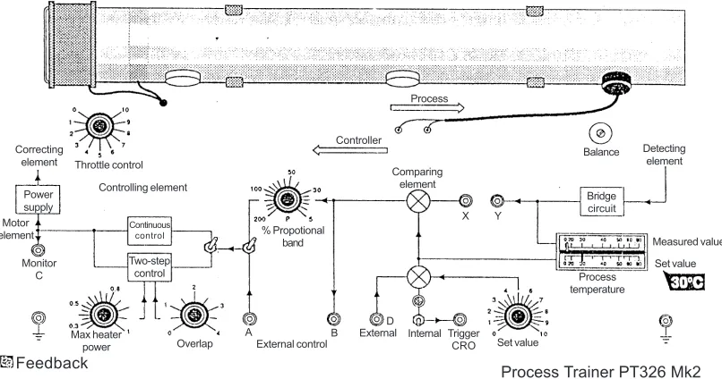
The PT326 process trainer, as shown in Figure 2, is a self-contained process and control equipment. In this equipment, air drawn from atmosphere by a centrifugal blower is driven past a heater grid and through a length of tubing to atmosphere again. The air stream velocity may be adjusted by means of an inlet throttle attached to the blower. The process consists of heating the air flowing in the tube to the desired temperature level and the purpose of the control equipment is to measure the air temperature, compare it with a value set by the user and generate a control signal which determines the amount of electrical power supplied to a correcting element. In this case, a heater mounted adjacent to the blower [5]. The desired temperature may be set in a range of 30 to 60°C.
2.0 EXPERIMENTAL SET-UP FOR OPEN-LOOP AND CLOSED-LOOP SETTING
For open-loop and closed-loop setting, a PRBS signal of 5 different lengths is injected to the process trainer. Autocorrelation of the input signal and cross-correlation of the input and output signal is performed using the Dynamic Signal Analyzer (HP35670A DSA). The correlograms from the DSA are used to determine the transfer functions model of the process trainer for open-loop and closed-loop setting.
At the same time, data for the input and output signal is captured simultaneously using PicoScope (ADC - 200/100) which enables the user to use the computer together
Figure 2 Process trainer Feedback
Process Trainer PT326 Mk2 Correcting
element
Power supply Motor element
Monitor C
Throttle control
Continuous control
Controlling element
Two-step control
Max heater
power Overlap External control
A B
% Propotional band
Controller
Comparing element
Process
D
X Y
External Internal
measuring element
Trigger CRO Set value
Balance Detecting element
Bridge circuit
Process temperature
with the Pico analog to digital converter (ADC) as an oscilloscope, a spectrum analyser, and a meter. PicoScope uses an ADC to take sequences of voltage measurements from one or more inputs. It then displays the data in one or more views. These views can present the data in several formats. The data obtained from the PicoScope is used to validate the transfer functions model obtained from the correlograms by using MATLAB.
2.1 Results and Analysis for Open-Loop Setting
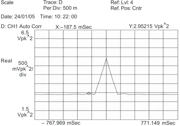
Figure 3 shows the autocorrelation of the input signal for N=127 for open-loop setting.
From Figure 3, the height of the ACF triangle, V2 = 2V and the bit interval is 0.12 s. The impulse strength is V2 times the bit interval which evaluates to 2.0 × 0.12 = 0.24Vs.
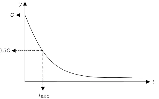
From Figure 4, the response appears to be an exponential graph that decays toward the value of 1.46V2. This value is minus from all the readings from the y-axis of the correlogram. Similarly, the graph seems to starts at 0.51s on the x-axis. So, 0.51s is deducted from all the readings from the x-axis. An expression of Ce–atcan be fitted to the curve as shown in Figure 5. From the curve, the transfer function model of the system can be determined by using Equation (3).
Figure 3 Autocorrelation of the input signal for N=127 for open-loop setting Ref: Lvl: 4
Ref. Pos: Cntr
6.5 Vpk ^2
Real
D: CH1 Auto Corr Scale
Date: 24/01/05 Time: 10: 22: 00 Trace: D Per Div: 500 m
X:–187.5 mSec Y:2.95215 Vpk^2
– 767.969 mSec 771.149 mSec
500 mVpk^2/
div
( )
(
)
( ) Ts
at
Ts e
G s L Ce
Ke G s
s a
ϕ
−
− −
−
=
= +
1
(3)
where,ϕ = bit interval × height of the ACF triangle and K =
ϕ
C
Figure 4 Cross-correlation of the input and output signal for N=127 for open-loop setting Ref: Lvl: 1.64
Ref. Pos: Cntr
1.84 Vpk^2
LinMag
C: Cross Corr2/1 Scale
Date: 24/01/05 Time: 10: 22: 00 Trace: C Per Div: 40 m
X: 500 mSec Y:1.79443 Vpk^2
– 767.969 mSec 5.001 Sec
40 mVpk^2
/div
1.44 Vpk^2
Figure 5 Approximation of the cross-correlogram for open-loop setting 0.5C
y
C
T0.5C
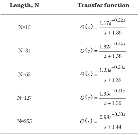
Table 2 Transfer function for each PRBS maximum length
Length, N Transfer function
N=15 ( )
. s . e G s s . − = + 0 52 1 17 1 39
N=31 ( )
. s . e G s s . − = + 0 54 1 32 1 58
N=63 ( )
. s . e G s s . − = + 0 53 1 23 1 39
N=127 ( )
. s . e G s s . − = + 0 51 1 35 1 36
N=255 ( )
. s . e G s s . − = + 0 50 0 99 1 44
Figure 5 shows an ideal cross-correlogram for a first order system using pseudo-random binary sequence as an input signal. The first peak value of the cross-correlogram is assumed as C. By substituting y = C, t = 0 and y = 0.5C, t = T0.5C into the expression y = Ce–at, and by taking natural logarithms:
. C . a T = 0 5 ln 0 5
(4)
From Figure 4, T0.5C= 0.53 s and C = 0.33 V2. Substituting T0.5C= 0.53 s into Equation (4) yields a = 1.31. The time delay is the time where the first peak occurs, which is 0.51 s. From Equation (3), the transfer function becomes:
( )
(
)
( ) . s . t . s eG s L . e
. . e G s s . − − − − = = + 0 51
1 1 31
0 51 0 33 0 24
1 38 1 31
Therefore, the average transfer function model for open-loop setting using 5 different lengths of PRBS is:
( ) . e . s
G s
s .
−
= +
0 52 1 23
1 42
2.2 Results and Analysis for Closed-loop Setting
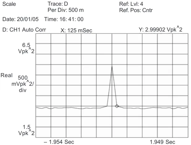
Figure 6 shows the autocorrelation of the input signal for N=127 for closed-loop setting.
From Figure 6, the height of the ACF triangle, V2 = 2V and the bit interval is 0.12 s. The impulse strength is V2 times the bit interval which evaluates to 2.0 × 0.12 = 0.24 Vs.
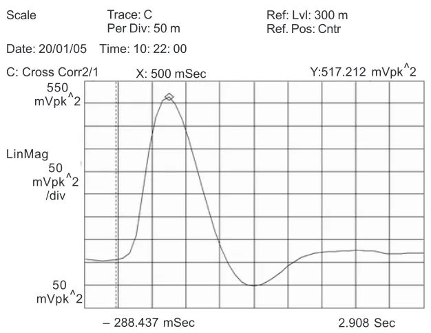
From Figure 7, the response appears to be a decaying sine wave. The sine wave settles at a value of 0.175 V2 . This value is minus from all the readings from the y-axis of the correlogram. Similarly, for the x-axis, the waveform seems to start at 0.14 s. Therefore, 0.14 s is deducted from all the readings from the x-axis. An expression of Ce–atsin–t can be fitted to the curve and by doing so, the transfer function of the system can be obtained using Equation (5):
Figure 6 Autocorrelation of the input signal for N =127 for closed-loop setting Ref: Lvl: 4
Ref. Pos: Cntr
6.5 Vpk^2
Real
D: CH1 Auto Corr Scale
Date: 20/01/05 Time: 16: 41: 00 Trace: D Per Div: 500 m
X: 125 mSec Y: 2.99902 Vpk^2
– 1.954 Sec 1.949 Sec
500 mVpk^2/
div
( ) e Ts
(
at)
G S = ϕ− L−1 Ce− sinωt (5)
where, ϕ = bit interval × height of the ACF triangle.
Figure 7 Cross-correlation of the input and output signal for N=127 for closed-loop setting Ref: Lvl: 300 m
Ref. Pos: Cntr
550 mVpk^2
LinMag
C: Cross Corr2/1 Scale
Date: 20/01/05 Time: 10: 22: 00 Trace: C Per Div: 50 m
X: 500 mSec Y:517.212 mVpk^2
– 288.437 mSec 2.908 Sec
50 mVpk^2
/div
50 mVpk^2
The model parameters can be calculated using the following steps:
(i) The graph has zero crossings at delays of 0.88 s and 1.80 s, giving two almost equal half-cycles averaging 0.92 s.
(ii) The cycle time is 2ωπ , and from Figure 7, 1.80 = 2ωπ and so ω =3 43. rad/s. (iii) The delay between the successive peaks are 0.92 s (half a cycle) apart. The height of the first positive peak is 0.35 V2 and the depth of the first negative peak is –0.08 V2. It is acceptable to consider one positive and one negative peak since the decay envelope is symmetrical about the zero amplitude
axis. Therefore, e–0.92a = .
. 0 08
0 35, and solving the equation, yields a =1.6 rad/s. (iv) The value of C can be obtained from the value of the cross-correlation halfway
of the equation, where 0.31 = Ce–0.46 × 1.6 and so C ≈ 0.65.
(v) The time delay, T, of the system is the delay of the first peak which is 0.46 s.
Plug in all the parameters obtained into Equation (5) and the resultant transfer function of the closed-loop system is:
( )
(
)
( )
( )
1 1 6
2 2
0 46 2
0 65 sin 3 43
0 24 1
0 24 2
9 29
3 20 14 32
Ts . t Ts n n n . s e
T s L . e . t
. C e T s . s . e T s
s . s .
ω ξω ω − − − − − = = × + + = + +
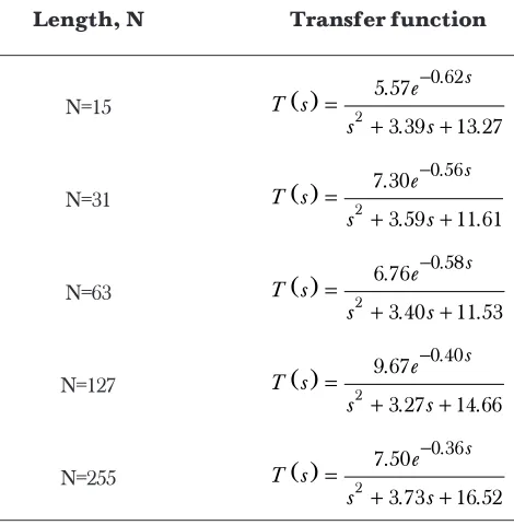
In this experiment, 5 maximum length sequence (MLS) of PRBS were used to identify the system. For each MLS, 3 samples of autocorrelation and cross-correlation graphs were taken for analysis. Table 3 shows the transfer function obtained using several different PRBS maximum length.
Therefore, the average transfer function model for closed-loop setting using 5 different length of PRBS is:
Table 3 Transfer function for each PRBS maximum length
Length, N Transfer function
N=15 ( ) 2
0 62
5 57
3 39 13 27
. s
. e T s
s . s .
−
=
+ +
N=31 ( ) 2
0 56
7 30
3 59 11 61
. s
. e T s
s . s .
−
=
+ +
N=63 ( ) 2
0 58
6 76
3 40 11 53
. s
. e T s
s . s .
−
=
+ +
N=127 ( ) 2
0 40
9 67
3 27 14 66
. s
. e T s
s . s .
−
=
+ +
N=255 ( ) 2
0 36
7 50
3 73 16 52
. s
. e T s
s . s .
−
=
( ) . e . s
T s
s . s .
−
=
+ +
0 50 2
7 36
3 48 13 52
3.0 MODEL VALIDATION
A total of 500 data was captured using PicoScope for the input and output signal of the process trainer for each sequence of PRBS. The data were used to plot the autocorrelation and cross-correlation graph for validation purposes. Figures 8 and 9 below show the PRBS input signal of N=127 and the output signal captured by the PicoScope for open-loop and closed-loop setting.
Figure 8 Input and output signal for open-loop setting using PRBS length of N=127 –3
ch A: Peak to peak ... 3150 ch B: Peak to peak ... 2132
24Jan2005 10:13 –5
5 V
3
1 –1
10 12 14
2
0 4 6 8
–3 –5 5 V
3
1 –1
16 18 20
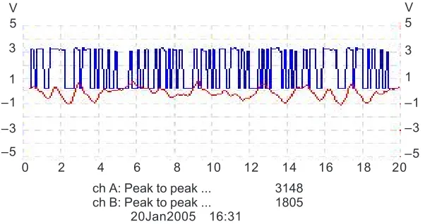
Figure 9 Input and output signal for closed-loop setting using PRBS length of N=127 –3
ch A: Peak to peak ... 3148 ch B: Peak to peak ... 1805
20Jan2005 16:31 –5
5 V
3
1 –1
10 12 14
2
0 4 6 8
–3 –5 5 V
3
1 –1
Please refer to Figures 10 and 11 for the lag index axis, where 1 unit of lag index represents 0.04 s. The correlograms obtained is similar to the one captured using Dynamic Signal Analyzer (DSA).
Figure 11 Cross-correlation graph plotted using MATLAB for open-loop setting using PRBS of length N=127
1.6 1.55 1.8
x 106
1.75 1.7 1.65
1.5 1.45 1.85
Lag index
Autocorrelation (microV
2 )
5 10 15 20 25 30 35 40
1.4 1.35 0
Figure 10 Autocorrelation graph plotted using MATLAB for open-loop setting using PRBS of length N=127
3
2.5 5
x 106
4.5
4 3.5
2 1.5 5.5
Lag index
Autocorrelation (microV
2 )
5 10 15 20 25 30 35 40
Please refer to Figures 12 and 13 for the lag index axis, where 1 unit of lag index represents 0.04 s. The correlograms obtained is similar to the one captured using
Figure 12 Autocorrelation graph plotted using MATLAB for closed-loop setting using PRBS of length N=127
3
2.5 5
x 106
4.5
4
3.5 5.5
Lag index
Autocorrelation (microV
olt
2 )
5 10 15 20 25
0
Figure 13 Cross-correlation graph plotted using MATLAB for closed-loop setting using PRBS of length N=127
3 2.5 5
x 105
4.5 4 3.5
1.5 1 5.5
Lag index
Cross-correlation (microV
olt
2 )
40
10 20 30 50 60
0.5 2
4.0 CONCLUSION
PRBS is a good choice when selecting input signal for system identification as it is easy to generate and introduce into a system. The constant _t avoids the distortion that occurs by attempting too rapid switching which is required with a completely random binary sequence. The signal intensity is low with energy spreading over a wide range of frequency that makes it suitable to force function for a plant operating normally, as it causes little disturbance from operating condition [6].
Table 4 shows the average transfer functions of PT326 process trainer for open-loop and closed-loop setting obtained using 5 different maximum length sequence of PRBS as input signal. The accuracy of the result can be improved by increasing the sequence of the PRBS being used and the bit interval must be carefully chosen so that the impulse response of the test system decays effectively to zero.
Table 4 Summary of the results obtained using cross-correlation technique
Open-loop Closed-loop
( ) . e . s
G s
s .
− =
+
0 52
1 23
1 42 ( ) 2
0 50
7 36
3 48 13 52
. s
. e T s
s . s .
−
=
+ +
REFERENCES
[1] Ogata, K. 1992. Systems Dynamics. USA: Prentice Hall.
[2] Franklin, G. F., J. D. Powell, and A. Emami-Naeini. 2002. Feedback Control of Dynamic Systems-Fourth Edition. USA: Prentice Hall.
[3] Pintelon, R., and J. Schoukens. 2001. System Identification: A Frequency Domain Approach. USA: IEEE Press. [4] Dutton, K., S. Thompson, and B. Barraclough. 1997. The Art of Control Engineering. Great Britain:
Addison-Wesley. 414-415, 420-422, 426-427.
[5] Feedback Instruments Limited. 1996. Process Trainer PT326. User Manual: Crowborough. 1-9.