NORLIZA BINTI ADNAN
COMPARING THREE METHODS OF HANDLING MULTICOLLINEARITY
USING SIMULATION APPROACH
NORLIZA BINTI ADNAN
A thesis submitted in fulfilment of the
requirements for the award of the degree of
Master of Science (Mathematics)
Faculty of Science
Universiti Teknologi Malaysia
To
My loving and supportive parents,
Hj Adnan and Pn Ramnah
My siblings,
Hairil, Aizam, Haffiz and Sarah
and
iv
ACKNOWLEDGEMENT
“I
n
the name od ALLAH the All-Merciful, The All-Compassionate. All praise be to
ALLAH
f
or
gi
v
i
ng
me
t
he
s
t
r
e
ngt
h
and
c
our
age
t
o
c
ompl
e
t
e
t
hi
s
t
he
s
i
s
”
A very great gratitude and appreciation expressed to all those who make a part to
the successful cease of this thesis either directly or indirectly. Particularly, I wish to
express my sincere appreciation to my main thesis supervisor, Dr. Maizah Hura binti
Ahmad, for encouragement, guidance, critics and motivation. I am also very thankful to
my co-supervisor Dr. Robiah binti Adnan for her guidance, advices and motivation.
Without their continued support and interest, this thesis would not have been the same as
presented here. An appreciation also goes to the Universiti Teknologi Malaysia for
financial support.
ABSTRACT
vi
ABSTRAK
TABLE OF CONTENTS
CHAPTER
SUBJECT
PAGE
COVER
i
DECLARATION
ii
DEDICATION
iii
ACKNOWLEDGEMENT
iv
ABSTRACT
v
ABSTRAK
vi
TABLE OF CONTENTS
vii
LIST OF TABLES
x
LIST OF FIGURES
xiv
LIST OF SYMBOLS
xvii
LIST OF APPENDICES
xix
1
INTRODUCTION
1.1
Background
1
1.2
The Problem of Multicollinearity
2
1.3
Statement of Problem
5
1.4
Research Objectives
5
1.5
Scope of Research
5
viii
2
LITERATURE REVIEW
2.1
Introduction
7
2.2
Ordinary Least Squares Regression
7
2.3
Multicollinearity Problem in Regression Analysis
10
2.3.1
Explanation of Multicollinearity
10
2.3.2
Effects of Multicollinearity in Least Squares
Regression
13
2.3.3
Multicollinearity Diagnostics
23
2.3.3.1 Informal Diagnostics
24
2.3.3.2 Formal Methods
25
2.4
Concluding Remarks
32
3
METHODS FOR HANDLING MULTICOLLINEARITY
3.1
Introduction
34
3.2
Partial Least Squares Regression
35
3.2.1
The construction of
k
components
37
3.2.2
Regress the response into
k
components
40
3.3
Principal Components Regression
49
3.3.1
The construction of
k
components
50
3.3.2
Regress the response into
k
components
53
3.3.3
Bias in Principal Components Coefficient
54
4
SIMULATION AND ANALYSIS
4.1
Introduction
71
4.2
Generating Simulated Data Sets
72
4.3
Performance Measures
76
4.4
Simulation Results
78
4.4.1
Partial Least Squares Regression
82
4.4.2
Principal Component Regression
104
4.4.3
Ridge Regression
116
5
COMPARISONS ANALYSIS AND DISCUSSIONS
5.1
Introduction
125
5.2
Performance on Classical Data
125
5.3
Performance on Simulated Data Sets
127
5.4
Comparison Analysis
134
5.5
Discussions
142
6
SUMMARY, CONCLUSIONS AND FUTURE RESEARCH
6.1
Introduction
145
6.2
Summary
145
6.3
Significant Findings and Conclusions
147
6.4
Future Research
149
x
LIST OF TABLES
TABLE NO.
TITLE
PAGE
3.1
Tobacco Data
45
3.2
Variance Inflation Factors for Tobacco Data
46
3.3
PLS weights vectors, rk
for the PLS Components
46
3.4
Loadings for the PLS Components
47
3.5
PLS Components
47
3.6
RMSE values for
k
components
48
3.7
MSE values for
k
components
49
3.8
The correlation matrix
58
3.9
The eigenvalues of the correlation matrix
58
3.10
Matrix of eigenvectors
58
3.11
The principal components
59
3.12
Values of
C
and the regression coefficients for various
values of
69
4.1
Factors and levels for the simulated data sets
72
4.2
The specific values for
x
ipfor each sets of
p
regressors
74
4.3
The response variable,
y
for each sets of
p
regressors
74
4.4
The
VI
F’
s
va
l
ue
s
f
or
t
he
c
hoi
c
e
of
t
he
va
r
i
a
nc
e
,
for noise
matrix (
)
75
4.9
Regression model for
p
= 2 regressors for
n =
100
80
4.10
Regression model for
p
= 4 regressors for
n
= 100
80
4.11
Regression model for
p
= 6 regressors for
n
= 100
81
4.12
PLS weights,
r
ifor the PLS Components for
p
= 2 regressors 83
4.13
PLS weights,
r
ifor the PLS Components for
p
= 4 regressors 83
4.14
PLS weights,
r
ifor the PLS Components for
p
= 6 regressors 83
4.15
PLS weights,
r
ifor the PLS Components for
p
=50 regressors 84
4.16
PLS loadings,
p
ifor the PLS Components for
p
=2 regressors 85
4.17
PLS loadings,
p
ifor the PLS Components for
p
=4 regressors 85
4.18
PLS loadings,
p
ifor the PLS Components for
p
=6 regressors 85
4.19
PLS loadings,
p
ifor the PLS Components for
p=50 regressors 86
4.20
Correlations between each PLS components and
y
87
4.21
Correlation between each components
89
4.22
RMSE values for
p
= 2 data sets
97
4.23
RMSE values for
p
= 4 data sets
97
4.24
RMSE values for
p
= 6 data sets for first five
PLS components
97
4.25
RMSE values for
p
= 50 data sets for first five
PLS components
97
4.26
Regression model using all the PLS Scores for
p =
2
and
n
= 100
99
4.27
Regression model using all the PLS Scores for
p =
4
and
n
= 100
100
4.28
Regression model using selected PLS Scores
for
p
= 4 (kopt
= 1)
101
4.29
Regression model using selected PLS Scores (
kopt
= 5 )
for
p =
6 and
n
= 100
102
4.30
The eigenvalues of the correlation matrix
105
4.31
Matrix of eigenvectors
106
4.32
Percentage of variance explained and the eigen values
xii
4.33
Percentage of variance explained and the eigen values
of the
p
= 4
108
4.34
Percentage of variance explained and the eigen values
of the
p
= 6
108
4.35
Percentage of variance explained and the eigen values
of the
p
= 50
109
4.36
Regression model using all the PC scores for
p =
2
and
n
= 100
111
4.37
Regression model using selected PC scores (PC
1) for
p =
2 and
n
= 100
111
4.38
Regression model using all the PC scores for
p =
4
and
n
= 100
112
4.39
Regression model using selected PC scores (PC
1) for
p =
4 and
n
= 100
113
4.40
Regression model using all the PC scores for
p =
6
and
n
= 100
114
4.41
Regression model using selected PC scores (PC
1) for
p =
6 and
n
= 100
114
4.42
Values of
,
C
and coefficient vectors employed for
p
= 2 and
n
= 100
119
4.43
Values of
,
C
and coefficient vectors employed for
p
= 4 and
n
= 100
120
4.44
Values of
,
C
and coefficient vectors employed for
p
= 6 and
n
= 100
121
5.1
Performance of PLS, PC and RR methods on
classical data sets
126
5.6
MSE values for
p
= 2 and specified
n
= 20, 30, 40, 60, 80
and 100
131
5.7
MSE values for
p
= 4 and specified
n
= 20, 30, 40, 60, 80
and 100
131
5.8
MSE values for
p
= 6 and specified
n
= 20, 30, 40, 60, 80
and 100
135
5.9
MSE values for
p
= 50 and specified
n
= 60, 80 and 100
135
5.10
Summary of the performances of the three methods
with
p
= 2
142
5.11
Summary of the performances of the three methods
with
p
= 4
142
5.12
Summary of the performances of the three methods
with
p
= 6
143
5.13
Summary of the performances of the three methods
xiv
LIST OF FIGURES
FIGURE NO.
TITLE
PAGE
1.1
Multicollinearity in simple linear regression
3
1.2
Multicollinearity in multiple linear regression
4
2.1
Picket Fences illustrations
15
2.2
The choice of VIF value against the R-square value.
29
3.1
Steps in SIMPLS algorithm
42
3.2
Steps in Principal Component Regression algorithm
56
3.3
The sampling distribution of biased and unbiased estimator
61
3.4
Steps in Ridge Regression algorithm
67
3.5
Plot of
C
against
70
4.1
Flowchart summarizing performance assessment
of methodology
77
4.2
Correlation between x1 and x2 for
p
= 2 regressors
88
4.3
Correlation between first and second components
for
p
= 2 regressors
89
4.4
Correlation between each components for
p
= 4 regressors
90
4.5
Correlation between each components for
p
= 6 regressors
92
4.6
X- and Y-scores for
p
= 2 regressors
(First and second components)
94
4.7
X- and Y-scores for
p
= 4 regressors (All components)
94
4.8
Correlation between first five components of
p
= 6
4.10
Plot of
against
C
for
p
= 4 and
n
= 100
117
4.11
Plot of
against
C
for
p
= 6 and
n
= 100
118
4.12
Plot of
against
C
for
p
= 50 and
n
= 100
118
5.1
Plot of regression coefficients against number of regressors
126
5.2
Plot of
R
2against
m
= 100 replications for
p
= 2 for
specified
n =
20
128
5.3
Plot of
R
2against
m
= 100 replications for
p
= 2 for
specified
n =
100
128
5.4
Plot of
R
2against
m
= 100 replications for
p
= 4 for
specified
n =
20
131
5.5
Plot of
R
2against
m
= 100 replications for
p
= 4 for
specified
n =
100
131
5.6
Plot of
R
2against
m
= 100 replications for
p
= 6 for
specified
n =
20
132
5.7
Plot of
R
2against
m
= 100 replications for
p
= 6 for
specified
n =
100
132
5.8
Plot of
R
2against
m
= 100 replications for
p
= 50 for
specified
n =
60
133
5.9
Plot of
R
2against
m
= 100 replications for
p
= 50 for
specified
n =
100
133
5.10
Plot of MSE values against
m
= 100 replications for
p
= 2 for
n =
20
138
5.11
Plot of MSE values against
m
= 100 replications for
p
= 2 for
n =
100
138
5.12
Plot of MSE values against
m
= 100 replications for
p
= 4 for
n =
20
139
5.13
Plot of MSE values against
m
= 100 replications for
p
= 4 for
n =
100
139
5.14
Plot of MSE values against
m
= 100 replications for
xvi
5.15
Plot of MSE values against
m
= 100 replications for
p
= 6 for
n =
100
140
5.16
Plot of MSE values against
m
= 100 replications for
p
= 50 for
n =
60
141
5.17
Plot of MSE values against
m
= 100 replications for
LIST OF SYMBOLS
y
Response (dependent) variable
x
Predictor (independent) variable
Parameter (regression coefficient), known constant
Error
2
Variance
Y
Matrix of observations
X
Matrix of predictors
β
Vector of parameters
ε
Vector of error matrix term
I
Identity matrix
ˆ
Estimate regression coefficient
β
ˆ
Vector of estimate regression coefficient
y
ˆ
Fitted value
H
Hat matrix
hii
ith diagonal element of hat matrix
e
Residual term
e
Vector of residual term
n
Number of observations
p
Number of regressors
Shrinkage parameter
xviii
P
Matrix of
x-loadings
r
PLS weight vectors
k
Number of components for PLS and PCR
R
2Coefficient of Determination
Z
Components for Principal Component Regression
ABBREVIATIONS
MEANING
CI
Condition Indices
cov
Covariance
GCV
Generalized Cross Validation
LS
Least Squares
max
Maximum
MSE
Mean Square Error
OLS
Ordinary Least Squares
PCR
Principal Component Regression
PLSR
Partial Least Squares Regression
RMSE
Root Mean Square Error
RR
Ridge Regression
xx
LIST OF APPENDICES
APPENDIX
TITLE
PAGE
A
S-PLUS codes for data generating function
156
B
S-PLUS codes and simulation results for Partial Least
Squares Regression method in Chapter IV
162
C
S-PLUS codes and simulation results for Principal
Component Regression method in Chapter IV
182
D
S-PLUS codes and simulation results for Ridge
Regression method in Chapter IV
200
E
S-PLUS code for classical data set
215
INTRODUCTION
1.1
Background
Regression analysis is one of the most widely use of all statistical tools that
utilizes the relation between two or more quantitative variables so that one variable can
be predicted from the others. The relationship of each predictor to the criterion is
measured by the slope of the regression line of the criterion
Y
on the predictor. The
regression coefficients are the values of these slopes.
The multiple linear regression model relates
Y
to
X
1,
X
2,...,
X
pand can be
expressed in terms of matrices as
y
X
β
ε
where
y
is the
nx1 vector of observed
response values,
X
is the
nxp
matrix of
p
regressors,
β
is the
px1 regression
2
linear regression model may be used to identify important regressor variables that can be
used to predict future values of the response variable.
The method of least squares is used to find the best line that on the average, is
closest to all points. In other words, to find the the best estimates of
’
s
wi
t
h
t
he
l
e
a
s
t
squares criterion which minimizes the sum of squared distances of all points from the
actual observation to the regression surface. The name least squares comes from
minimizing the squared residuals. From the Gauss-Markov theorem, least squares is
always the best linear unbiased estimator (BLUE) and if
is assumed to be normally
distributed with mean 0 and variance
2, then least squares is the uniformly minimum
variance unbiased estimator.
1.2
The Problem of Multicollinearity
In the applications of regression analysis, multicollinearity is a problem that
always occurs when two or more predictor variables are correlated with each other. This
problem can cause the value of the least squares estimated regression coefficients to be
conditional upon the correlated predictor variables in the model. As defined by
Bowe
r
ma
n
a
nd
O’
Conne
l
l
(
1990)
,
mul
t
i
c
ol
l
i
ne
a
r
i
t
y
i
s
a
pr
obl
e
m
i
n
r
egr
e
s
s
i
on
a
na
l
ys
i
s
when the independent variables in a regression model are intercorrelated or are dependent
on each other.
using some method of estimation or some modifications of the method of least squares
for estimating the regression coefficients.
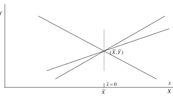
The problem of multicollinearity can occur in both simple linear regression and
multiple linear regression. Figure 1.1 illustrates the problem of multicollinearity that
occur in simple regression (Wannacott and Wannacott, 1981). The figure shows how the
estimate
ˆbecomes unreliable if the
Xi
’
s
wer
e
c
l
os
e
l
y
bunc
he
d,
t
ha
t
i
s
,
i
f
t
he
r
e
gr
e
s
s
or
X
had little variation. When the
Xi
’
s
a
r
e
c
onc
e
nt
r
a
t
e
d
on
one
s
i
ngl
e
va
l
ue
X, then
ˆis not
determined at all. For each line, the sum of squared deviations is the same, since the
deviations are measured vertically from
(X,Y). If
Xi X, then all
xi
= 0, and the term
involving
β
ˆ
is zero. Hence, the sum of squares does not depend on
β
ˆ
at all. Therefore,
when the values of
X
show little or no variation, then the effect of
X
on
Y
can no longer
be sensibly investigated. The best fit for
Y
for data with multicollinearity was not a line,
but rather a point
(X,Y). In explaining
Y, multicollinearity makes the
X
i’
s
l
os
e
one
dimension.
Figure 1.1
:
Multicollinearity in simple regression
X0
x