ABSTRACT
JADOUN, FADI MUNIR. Calibration of the Flexible Pavement Distress Prediction Models in the Mechanistic Empirical Pavement Design Guide (MEPDG) for North Carolina. (Under the direction of Y. Richard Kim).
Roadway pavement structures in the United States have been designed over the last several decades using empirical-based procedures that were developed using performance data measured in the 1950s at the AASHO road test in Ottawa, Illinois. Because of the significant changes in truck axle loads and configurations, truck tire pressure, construction practices and materials, in addition to climate and subgrade soil differences from one location to another, these empirical design procedures have become unsuitable for the current design of new and rehabilitated pavement structures. Due to the limitations of the empirical-based pavement design procedures, the AASHTO Joint Task Force on pavements initiated an effort in 1996 to develop an improved pavement design guide that employs existing state-of-the-practice mechanistic-based models and design procedures. The product of this initiative became available in 2004 in the form of software called the Mechanistic-Empirical Pavement Design Guide (MEPDG). The mechanistic component of the MEPDG calculates pavement critical responses based on layer material properties and traffic loading. The empirical component bridges the gap between laboratory and field performance.
The performance prediction models in the MEPDG were calibrated and validated using performance data measured for hundreds of sections across the United States.
However, these nationally calibrated models do not necessarily reflect local materials, local construction practices, and local traffic characteristics. This dissertation focuses on North Carolina pavement structures, for which the nationally calibrated models do not lead to accurate pavement designs, as was found from verification work. The MEPDG distress prediction models must be recalibrated using local materials, traffic, and environmental data. Realizing the huge impact of traffic on pavement performance, it is also necessary to
The work presented in this dissertation focuses on four major topics: 1) the permanent deformation (or so-called rutting) performance characterization of twelve asphalt mixtures commonly used in North Carolina; 2) recalibration of the flexible pavement distress prediction models in the MEPDG to reflect local materials and conditions; 3) the
development of a GIS-based methodology to enable the extraction of local subgrade soils data from a national soils database; and 4) the unique characterization of local North Carolina traffic while considering the effect of traffic on pavement performance.
For the rutting performance characterization, triaxial repeated load permanent deformation (TRLPD) confined tests are performed, and material-specific rutting model coefficients for twelve common asphalt mixtures are developed. In order to calibrate the rutting prediction model coefficients, two optimization approaches are evaluated; one uses the generalized reduced gradient (GRG) method, and the other uses a genetic algorithm (GA) optimization technique. For the subgrade materials, a GIS-based methodology is developed to take advantage of the NCHRP 9-23A national soils database. The method allows any road section in North Carolina to be superimposed accurately onto pre-developed soil maps. Regarding traffic characterization, the MEPDG is employed to develop damage factor regression models to estimate the relative damage caused by 140 axle type/load
combinations. Damage factors are essential for proper clustering of multiple MEPDG traffic inputs.
Calibration of the Flexible Pavement Distress Prediction Models in the Mechanistic Empirical Pavement Design Guide (MEPDG) for North Carolina
by
Fadi Munir Jadoun
A dissertation submitted to the Graduate Faculty of North Carolina State University
in partial fulfillment of the requirements for the degree of
Doctor of Philosophy
Civil Engineering
Raleigh, North Carolina 2011
APPROVED BY:
________________________ ________________________ Y. Richard Kim, Professor John R. Stone, Professor Chair of Advisory Committee
________________________ ________________________ Roy H. Borden, Professor S. Ranji Ranjithan, Professor
ii
DEDICATION
To my wonderful and precious wife, Nivine, and to my sons, Munir-Jeremy (MJ) and
Martin, I dedicate the fruit of four and a half years of hard work, my dissertation. It is
because of the Lord and your love and inspiration that I was able to finish this work and earn my degree. I love you Nivine because of who you are: loving, gentle, caring, tender,
forgiving, very patient, supportive, and a great cook. On top of all that, you are so beautiful and talented. I thank the Lord for He gave me such a great wife and sons. I love you MJ
because I see my childhood in you; I love the way you hold your guitar, and your hand tools, and I love the accent in which you pronounce words, I just love everything about you. I cannot forget the day you were born, I had my first final exam during the first semester in my Ph.D. program. Nevertheless, I enjoyed being with you and Mom. I love you MJ, I love you
so much. I pray that you might be inspired by your dad’s achievements and do more, much more. As for you Martin, you little smart troublemaker! you are now one and a half years
old, you talk like a three year old. I love the falcon-sharp eyes you have and the way you look at others. I love your big tummy and your smile. I have not discovered your talents yet, other than rocking whenever you hear music, but I am working on it. I love you Martin and I
pray that you will also be inspired and achieve a lot in your life. Achievements that can positively touch the lives of others around you.
I also dedicate this work to my parents, Munir and Mary, my brother, Ehab, and sisters, Carmen and Katia, and to my in-laws for their unfailing love, support, and
iii
BIOGRAPHY
iv
ACKNOWLEDGEMENTS
“1The heavens declare the glory of God; the skies proclaim the work of his
hands.2Day after day they pour forth speech; night after night they reveal knowledge.3They
have no speech, they use no words; no sound is heard from them. 4Yet their voice goes out
into all the earth, their words to the ends of the world. In the heavens God has pitched a tent
for the sun. 5It is like a bridegroom coming out of his chamber, like a champion rejoicing to
run his course.6It rises at one end of the heavens and makes its circuit to the other; nothing is
deprived of its warmth.”–Psalm 19:1-9
God is the creator of everything and He is the source of all knowledge and true
wisdom. I realize that the wisdom we need most cannot be acquired through science, philosophy, or the arts. True wisdom comes only from God, by revelation. “If any of you
lacks wisdom, let him ask of God” (James 1:5). I declare that without Him, I would not have accomplished this work. I am thankful to Him for the privilege of seeing a glimpse of his marvelous power and magnificent design through my research.
I would like to acknowledge my advisor, Dr. Y. Richard Kim, for his continuous support and friendship. I would like to thank my committee members: Dr. John Stone, Dr. Roy Borden, and Dr. Ranji Ranjithan for their invaluable recommendations. Special thanks to Shane Underwood for the technical assistance he consistently provided. I extend my thanks to current and former group members: Yeongtae Choi, Andrew LaCroix, Cheolmin Baek, Tian Hou, and Naresh Muthadi for their support. I also thank Fatemeh Sayyady for her technical input and enjoyable teamwork environment. Special thanks to Diane Gilmore for her continuous administrative support and encouragement throughout my program. Thanks to Jake Rhoads for opening his machine shop for me anytime I needed it.
Last but not least, I would like to thank the North Carolina Department of
v
TABLE OF CONTENTS
LIST OF TABLES...VIII LIST OF FIGURES ... XII LIST OF ACRONYMS ... XVII
CHAPTER 1 INTRODUCTION ...1
1.1 Background...1
1.2 Research Needs and Significance ...2
1.3 Research Objective ...3
1.4 Dissertation Organization ...4
CHAPTER 2 MATERIALS ACQUISITION...6
2.1 Identification of Twelve Most Commonly used Asphalt Mixtures in North Carolina....6
2.2 NCDOT Asphalt Mixture Designations ...6
CHAPTER 3 MIXTURE VERIFICATION PROCEDURE AND TARGET AIR VOIDS DEVELOPMENT...9
3.1 Introduction...9
3.2 Mixture Verification Procedure ...9
3.2.1 Development of a Mix Verification Acceptance Criteria ...10
3.2.2 Wet Sieve Analysis ...13
3.2.3 Measurement of Aggregate Dry Bulk-Specific Gravity (Gsb) ...15
3.2.4 Reclaimed Asphalt Pavement (RAP) Materials...17
3.2.5 Mixture Verification Results...18
3.3 Selection of a Target Air Void Percentage for Performance Test Specimens...19
CHAPTER 4 UNBOUND MATERIALS CHARACTERIZATION ...22
4.1 Introduction...22
4.2 GIS-Based Implementation Methodology for the NCHRP 9-23A Recommended Soil Parameters for Use as Input to the MEPDG...22
4.2.1 Introduction...22
4.2.2 Problem Statement ...24
4.2.3 Objective and Scope...24
4.2.4 MEPDG Unbound Materials Hierarchical Input Levels...25
4.2.5 Soil Water Characteristics Curve (SWCC)...26
4.2.6 Methodology to Superimpose Road Sections on NCHRP 9-23A Soil Maps ...27
CHAPTER 5 PERMANENT DEFORMATION AND FATIGUE DAMAGE CHARACTERIZATION...35
5.1 Permanent Deformation...35
vi
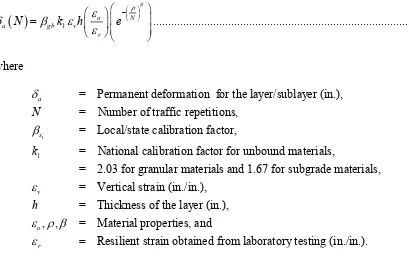
5.1.2 Rutting in the MEPDG...36
5.1.3 Test Equipment ...40
5.1.4 Triaxial Stress State ...40
5.1.5 TRLPD Test Temperatures ...43
5.1.6 TRLPD Test Results ...43
5.1.7 Rutting Characterization for the Twelve Most Commonly used Asphalt Mixtures in North Carolina...54
5.2 Fatigue Cracking...79
5.2.1 Introduction...79
5.2.2 Alligator Cracking in the MEPDG ...81
5.2.3 Fatigue Characterization for the Twelve Most Commonly used Asphalt Mixtures in North Carolina...82
CHAPTER 6 CHARACTERIZATION OF NORTH CAROLINA TRAFFIC FOR THE MEPDG...86
6.1 Introduction...86
6.2 A Comprehensive List of Traffic Input Parameters Required by the MEPDG ...87
6.3 Hierarchical Traffic Data Input Levels...88
6.4 Traffic Volume Adjustment Factors ...89
6.4.1 Monthly Adjustment Factors (MAF) ...91
6.4.2 Vehicle Class Distribution Factors (VCD) ...92
6.4.3 Hourly Distribution Factors (HDF) ...94
6.4.4 Traffic Growth Functions and Growth Rates...95
6.5 Axle Load Distribution Factors (ALDF) ...96
6.6 Role of Each Traffic Parameter in the Overall Analysis Process ...97
6.7 North Carolina Traffic Characterization Elements...99
6.7.1 Damage-Based Sensitivity Analysis ...105
6.7.2 Clustering Analysis to Guide the Development of ALDF...111
CHAPTER 7 LOCAL CALIBRATION OF THE MEPDG FLEXIBLE PAVEMENT PERFORMANCE PREDICTION MODELS ...129
7.1 Introduction...129
7.2 Overview of the MEPDG Analysis and Design Process ...129
7.3 MEPDG Calibration Terminology...131
7.3.1 Reliability...131
7.3.2 Model Verification...132
7.3.3 Model Calibration ...132
7.3.4 Ratio of the Standard Deviation of the Residual Error (Se) to the Standard Deviation of the Measured Performance (Sy): (Se/Sy) ...133
7.3.5 Model Validation ...134
7.3.6 Hierarchical Materials Data Input Levels ...134
7.4 Local Calibration Procedure, as Recommended by NCHRP 1-40B ...136
7.4.1 Background ...136
vii
7.5 Verification and Paper-Based Calibration Results using Level 3 Materials Data...147
7.6 Local Calibration Procedure for Rutting and Alligator Cracking Prediction Models in the MEPDG ...148
7.6.1 Background and Assumptions ...148
7.6.2 Hybrid MEPDG Version for Local Calibration...150
7.6.3 Rutting Models Calibration-Approach I-R ...150
7.6.4 Alligator Cracking Model and Transfer Function Calibration - Approach I-F...161
7.6.5 Validation of Rutting and Alligator Cracking Calibrated Models for Approach I ...171
7.6.6 Rutting Models Calibration-Approach II-R...176
7.6.7 Alligator Cracking Model and Transfer Function Calibration - Approach II-F...188
7.6.8 Validation of Rutting and Alligator Cracking Calibrated Models for Approach II ...198
7.6.9 Comparison between Approach I and Approach II and the Final Selection...204
CHAPTER 8 CONCLUSIONS AND RECOMMENDATIONS ...220
8.1 Conclusions...220
8.2 Recommendations...224
8.2.1 Recommendations for Future Enhancements ...224
8.2.2 Recommendations for Agencies Performing MEPDG Local Calibration Research ...226
REFERENCES ...228
APPENDICES ...233
Appendix A Local Calibration Sites Database ...234
Appendix B Dynamic Modulus (│E*│) Database...274
Appendix C Complex Shear Modulus (│G*│) Database ...278
Appendix D Permanent Deformation (Rutting) Database...280
Appendix E NC Subgrade Soils Database Extracted from NCHRP 9-23A ...360
viii
LIST OF TABLES
Table 2.1. Summary of the Twelve Most Commonly Used HMA Mixes in North
Carolina... 7
Table 2.2. Recommended Superpave HMA Mix Types Based on Traffic Levels ... 8
Table 3.1. NCDOT Control Limits for Mix Production ... 10
Table 3.2. NCDOT Assessment Program Criteria... 11
Table 3.3. AASHTO Materials Reference Laboratory Multi-laboratory Precision Limits... 11
Table 3.4. Mix Verification Criteria Developed for Local Calibration Project... 12
Table 3.5. Mix Verification Criteria for the Twelve Most Commonly used Mix Types in NC ... 12
Table 3.6 Combined Aggregate Gradations Obtained from Wet Sieve Analysis vs. JMF... 13
Table 3.7. Percentage Differences between JMF and Measured Combined Gradations... 14
Table 3.8. Change in Dry Bulk-Specific Gravity (Gsb) Over Time ... 16
Table 3.9. Effect of the Change in Dry Bulk-Specific Gravity on HMA Mix Volumetrics... 17
Table 3.10. Summary of Asphalt Binder Content for HMA Mixes with RAP... 18
Table 3.11. One-Point Mix Verification Test Results ... 19
Table 3.12. Four-Point Mix Design Test Results and Recommended Asphalt Contents ... 19
Table 3.13. Changes in Air Void Levels over Time – Results from 16 States... 20
Table 3.14. Project NCHRP 9-9 Average In-Place Air Voids... 21
Table 4.1. EICM Data Requirements for Unbound Materials Hierarchical Input Levels... 25
Table 4.2. Comparison between Soil Classifications from the NCHRP 9-23A Project and the LTPP Database ... 32
Table 5.1. NCHRP 9-30A Proposed Test Matrix for Repeated Load Testing Program... 41
ix
Table 5.3. Mixture Ranking Based on Permanent-to-Resilient Strain Ratio
(Worst to Best)... 46
Table 5.4. Effects of Different Optimization Methods on Rutting k Values for the S9.5B Mixture... 62
Table 5.5. Back-Calculated Rutting Material-Specific k Values for Some MnRoad Mixtures... 64
Table 5.6. Comparison of Rutting Model Coefficients among MEPDG, ASU, and NCSU Results ... 65
Table 5.7. Effect of Including 20°C TRLPD Test Data on S9.5B Rutting Model Coefficients... 67
Table 5.8. Effect of Including 20°C TRLPD Test Data on Predicted Rut Depth for Different Pavement Sections with the S9.5B Mixture in Different Environments... 69
Table 5.9. Effect of Using MEPDG Default Rutting k Values on Predicted Rut Depth for Different Pavement Sections with the S9.5B Mixture in Different Environments ... 69
Table 5.10. Effect of 20°C TRLPD Test Data on Mixture Ranking Based on Predicted Permanent Strain (εp) ... 73
Table 5.11. Effect of 20°C TRLPD Test Data on Mixture Ranking Based on Predicted Permanent-to-Resilient Strain Ratios (εp/εr) ... 74
Table 5.12. Effect of 20°C TRLPD Test Data on Percent Difference Between Measured and Predicted Permanent Strain (εp) and Permanent-to-Resilient Strain Ratios (εp/εr) ... 77
Table 5.13. Summary of the Rutting Model Material-Specific k Values for the MEPDG ... 78
Table 5.14. Summary of Fatigue Performance Rankings using Direct Tension vs. Beam Fatigue Simulations... 85
Table 5.15. Summary of the Fatigue Model Material-Specific k Values for as determined from Direct Tension Fatigue Simulation (psi-based) ... 85
Table 6.1. Traffic Input Parameters Required by the MEPDG... 88
Table 6.2. NCDOT Sensitivity Criteria for Flexible and JPCP Pavements... 106
Table 6.3. Sensitivity of Flexible Pavements to Different Traffic Parameters... 110
Table 6.4. Statistics of the Slope and Intercept for Linear Functions Representing Light and Heavy Axles ... 121
Table 6.5. Example Summary of Damage Factors Developed for WIM Site 525 ... 124
x
Table 7.2. Average Aggregate Gradation Measures for the Twelve Most
Commonly Used Mixtures in North Carolina... 145 Table 7.3. Asphalt Concrete Mixture Conversion List ... 147 Table 7.4. Complete List of βr2, and βr3 Combinations Used in Approach I-R
Calibration ... 151 Table 7.5. Preliminary Local Calibration Factors for HMA and Unbound
Rutting Prediction Models using Approach I-R ... 157 Table 7.6. Summary of Rutting Distress Statistical Parameters Before and After
Calibration using Approach I-R... 157 Table 7.7. Predicted Mean Rut Depth Before and After Calibration using
Approach I-R ... 160 Table 7.8. Complete List of βf2, and βf3 Sets Used in the Calibration Process... 166
Table 7.9. Preliminary Local Calibration Factors for Alligator Cracking
Prediction Models using Approach I-F... 168 Table 7.10. Summary of Alligator Cracking Statistical Parameters Before and
After Calibration using Approach I-F... 168 Table 7.11. Predicted and Measured Alligator Cracking Means, Before and After
Calibration using Approach I-F ... 169 Table 7.12. Comparison of Rutting Statistical Parameters between Approach I-R
Calibration and Validation... 172 Table 7.13. Comparison of Predicted Total Rut Depth between Approach I-R
Calibration and Validation... 173 Table 7.14. Comparison of Alligator Cracking Statistical Parameters between
Approach I-F Calibration and Validation ... 174 Table 7.15. Comparison of Predicted Alligator Cracking between Approach I-F
Calibration and Validation... 175 Table 7.16 Preliminary Local Calibration Factors for HMA and Unbound
Rutting Prediction Models using Approach II-R... 185 Table 7.17. Summary of Rutting Distress Statistical Parameters Before and After
Calibration using Approach II-R ... 185 Table 7.18. Predicted Mean Rut Depth Before and After Calibration using
Approach II-R ... 188 Table 7.19 Preliminary Local Calibration Factors for Alligator Cracking Model
xi
Table 7.20. Summary of Alligator Cracking Statistical Parameters Before and
After Calibration using Approach II-F ... 197 Table 7.21. Predicted and Measured Alligator Cracking Means, Before and After
Calibration using Approach II-F... 197 Table 7.22. Comparison of Rutting Statistical Parameters between Approach II-R
Calibration and Validation... 199 Table 7.23. Comparison of Predicted Total Rut Depth between Approach II-R
Calibration and Validation... 201 Table 7.24. Comparison of Alligator Cracking Statistical Parameters between
Approach II-F Calibration and Validation... 202 Table 7.25. Comparison of Predicted Alligator Cracking between Approach II-F
Calibration and Validation... 202 Table 7.26. Comparison between Local Calibration Factors from Approach I
and II... 204 Table 7.27. Comparison between Predicted and Measured Rut Depth and
Alligator Cracking from Approach I and Approach II ... 207 Table 7.28. Comparison of Approaches I and II Calibration Statistics to Default
Statistics... 208 Table 7.29. Total SSE Reported as Error per Field Measurement for Total Rut
Depth and Alligator Cracking... 209 Table 7.30. Comparison between Mean Predicted Total Rut and Alligator
Cracking from Approach I and Approach II for Validation and
Calibration Sections... 211 Table 7.31. Comparison between Total Rut and Alligator Cracking Calibration
and Validation Statistics from Approach I and Approach II ... 213 Table 7.32. Reasonableness Check of HMA Rutting Local Calibration Factors
Developed from Approach I and Approach II ... 215 Table 7.33. Reasonableness Check of Unbound Materials Rutting Local
Calibration Factors Developed from Approach I and Approach II ... 215 Table 7.34. Reasonableness Check of Alligator Cracking Local Calibration
Factors Developed from Approach I and Approach II ... 217 Table 7.35. Final Recommended Local Calibration Factors for the Rutting
Prediction Models... 218 Table 7.36. Final Recommended Local Calibration Factors for the Alligator
xii
LIST OF FIGURES
Figure 4.1. Example of a soil water characteristics curve... 27 Figure 4.2. A screen capture of the MEPDG EICM soils data generator. ... 30 Figure 5.1. Example of a severe permanent deformation case in flexible
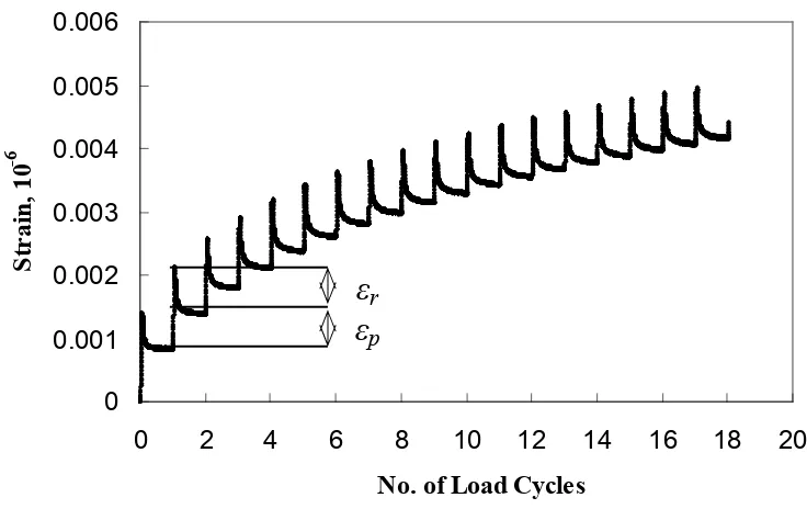
pavement... 35 Figure 5.2. Typical TRLPD permanent strain vs. number of cycles graph in
arithmetic scale. ... 38 Figure 5.3. Typical TRLPD permanent strain vs. number of cycles graph in
log-log scale. ... 38 Figure 5.4. Typical TRLPD recorded strain vs. number of cycles during the
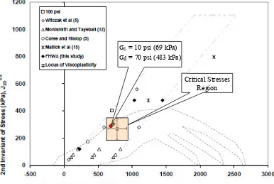
primary stage... 39 Figure 5.5 Critical stress region, as identified from the 3D viscoplastic model
analysis of KENLAYER. (Figure from Gibson et al. 2009). ... 42 Figure 5.6. Average permanent strain vs. number of cycles at 20°, 40°, and 54°C... 44 Figure 5.7. Average permanent-to-resilient strain ratio vs. number of cycles
at 20°, 40°, and 54°C. ... 45 Figure 5.8. Final permanent strain values and permanent-to-resilient strain ratios
at 20°, 40°, and 54°C. ... 47 Figure 5.9. Effect of temperature and binder grade on permanent strain: (a)
numerical difference; and (b) percent difference... 49 Figure 5.10. Effect of number of gyrations and specimen air void content on
permanent strain... 51 Figure 5.11. Effect of aggregate surface texture and percentage of flat and
elongated aggregate on permanent strain... 53 Figure 5.12. Approach followed for finding the rutting model coefficients: (a)
Log(εp/εr) vs. Log (N)relationship; and (b) Log(A) vs. Log(T)
relationship... 55 Figure 5.13. Comparison between predicted and lab-measured permanent strain
values for the S9.5B mixture: (a) arithmetic scale; and (b) logarithmic
scale. ... 57 Figure 5.14. Schematic diagram showing the two approaches for finding rutting k
values. ... 58 Figure 5.15. Pavement sections used in MEPDG simulation runs to check the
xiii
Figure 5.16. Effect of including 20°C data on predicted rut depth in thin and thick
pavements in three temperature zones. ... 70
Figure 5.17. Effect of using the national default rutting k values compared to NCSU lab-generated k values on rutting predicted by the MEPDG... 70
Figure 5.18. Effect of 20°C TRLPD test data on predicted permanent strain values (εp) and permanent-to-resilient strain ratios (εp/εr) compared to the measured values... 76
Figure 5.19. Real images of alligator cracking and longitudinal cracking. ... 80
Figure 6.1 FHWA vehicle classification scheme F report (courtesy of the FHWA). ... 90
Figure 6.2. A screen capture of the MEPDG monthly adjustment factors (MAF) window... 91
Figure 6.3. A screen capture of the MEPDG vehicle class distribution (VCD) factors window... 92
Figure 6.4. A screen capture of the available truck traffic classification (TTC) schemes window in the MEPDG... 93
Figure 6.5. A screen capture of the MEPDG hourly distribution factors (HDF) window... 94
Figure 6.6. A screen capture of the traffic vehicle class-specific growth factors window... 95
Figure 6.7. A screen capture of the MEPDG axle load distribution factors (ALDF) window. ... 96
Figure 6.8. Role of traffic parameters in the MEPDG structural analysis. ... 98
Figure 6.9. Comprehensive flowchart for the traffic characterization approach. ... 101
Figure 6.10. A screen capture of the VCD Generator and ALDF Cluster Selector tool. ... 104
Figure 6.11. Sensitivity analysis results of HDF for flexible pavements... 108
Figure 6.12. Sensitivity analysis results of MAF for flexible pavements. ... 108
Figure 6.13. Sensitivity analysis results of VCD for flexible pavements. ... 109
Figure 6.14. Sensitivity analysis results of ALDF for flexible pavements. ... 109
Figure 6.15. Results of four-dimensional ALDF clustering analysis... 113
Figure 6.16. Adjustments made to AADTT and general inputs for damage factors study... 117
xiv
Figure 6.18. Adjustments made to APT for damage factors study. ... 118 Figure 6.19. Adjustments made to ALDF for damage factors study. ... 119 Figure 6.20. Damage factors from site 525: (a) partial results of actual MEPDG
runs; (b) bilinear fitting functions; and (c) complete results of damage
factors... 122 Figure 6.21. ESAL-based damage factors developed using the MEPDG... 125 Figure 6.22. Average frequency of single, tandem, tridem, and quad axles from 44
WIM sites... 126 Figure 6.23. Combined effects of damage factors and frequency for different axle
type/load combinations... 127 Figure 6.24. Final results of two-dimensional ALDF clustering analysis. ... 128 Figure 7.1. Flowchart showing an overview of the MEPDG analysis/design
process. ... 130 Figure 7.2. Calibration/validation sections available for local calibration in North
Carolina... 139 Figure 7.3. Flowchart showing the major steps for calibrating the rutting models
under Approach I-R. ... 153 Figure 7.4. 3D surface of Total SSE between predicted and measured total rut
depth values for 110 combinations of βr2and βr3... 155
Figure 7.5. Total rut: (a) before calibration; and (b) after calibration using
Approach I-R. ... 159 Figure 7.6. Estimated measurement of AC rut depth: (a) before calibration; and
(b) after calibration using Approach I-R... 159 Figure 7.7. Estimated measurement of base rut depth: (a) before calibration; and
(b) after calibration using Approach I-R... 160 Figure 7.8. Estimated measurement of subgrade rut depth: (a) before calibration;
and (b) after calibration using Approach I-R... 160 Figure 7.9. Flowchart showing the major steps for calibrating the fatigue
cracking model and transfer function under Approach I-F... 162 Figure 7.10. 3D surface of SSE between predicted and measured alligator cracking
values for 187 combinations of βf2 and βf3. ... 167
Figure 7.11. Alligator cracking calibration results: (a) before calibration; and (b)
after calibration using Approach I-F... 170 Figure 7.12. Histogram for the distribution of measured percent alligator cracking
xv
Figure 7.13. Predicted vs. measured rut depth after validation work using
Approach I-R: (a) total rut; (b) estimated AC rut; (c) estimated base
rut; and (d) estimated subgrade rut. ... 173 Figure 7.14. Predicted vs. measured alligator cracking values after validation work
using Approach I-F. ... 176 Figure 7.15 Optimization steps of rutting model coefficients using Approach II-R... 178 Figure 7.16 Example of initial range and absolute boundaries setup for rutting
optimization – Approach II-R... 181 Figure 7.17. Change in total rut depth fitting function with number of individuals. ... 182 Figure 7.18. Total rut depth optimization progression from different GA runs... 183 Figure 7.19. Total rut depth: (a) before calibration; and (b) after calibration using
Approach II-R. ... 187 Figure 7.20. Estimated measurement of AC rut depth: (a) before calibration; and
(b) after calibration using Approach II-R. ... 187 Figure 7.21. Estimated measurement of base rut depth: (a) before calibration; and
(b) after calibration using Approach II-R. ... 187 Figure 7.22. Estimated measurement of subgrade rut depth: (a) before calibration;
and (b) after calibration using Approach II-R. ... 188 Figure 7.23 Optimization steps of fatigue models’ coefficients using
Approach II-F. ... 190 Figure 7.24 Example of initial range and absolute boundaries setup for alligator
cracking optimization – Approach II-F. ... 192 Figure 7.25 Change in total alligator cracking fitting function with number of
individuals... 194 Figure 7.26. Total alligator cracking optimization progression from different
GA runs... 195 Figure 7.27. Alligator cracking calibration results: (a) before calibration; and (b)
after calibration using Approach II-F. ... 198 Figure 7.28. Predicted vs. measured rut depth after validation work using
Approach II-R: (a) total rut; (b) estimated AC rut; (c) estimated base
rut; and (d) estimated subgrade rut. ... 200 Figure 7.29. Predicted vs. measured alligator cracking values after validation work
using Approach II-F... 203 Figure 7.30. Comparison between calibration results from Approach I and
Approach II: (a) predicted vs. measured total rut depth; and (b)
xvi
Figure 7.31. Comparison between validation results from Approach I and Approach II: (a) predicted vs. measured total rut depth; and (b)
xvii
LIST OF ACRONYMS
Acronym Meaning
AADTT Annual Average Daily Truck Traffic
AASHTO American Association of State Highway and Transportation Officials
ABC Aggregate Base Course
AC Asphalt Concrete
ALDF Axle Load Distribution Factors
APT Number of Axles per Truck
ATB Asphalt Treated Base
AVC Automatic Vehicle Classification
CTB Cement Treated Base
DARWin-ME Design, Analysis and Rehabilitation for Windows-Mechanistic Empirical
|E*| Dynamic modulus of asphalt concrete EICM Enhanced Integrated Climatic Model FHWA Federal Highway Administration
│G*│ Complex shear modulus of asphalt binder
GIS Geographic Information System
GUI Graphical User Interface HDF Hourly Distribution Factors
HMA Hot Mix Asphalt
IRI International Roughness Index
LDF Lane Distribution Factor
LOE Line of Equality
M&T Unit Materials and Tests Unit
MAF Monthly Adjustment Factors
MEPDG Mechanistic Empirical Pavement Design Guide
NMAS Nominal Maximum Aggregate Size
NRCS National Resources Conservation Service
PMS Pavement Management Systems
PMU Pavement Management Unit
SI Serviceability Index
SWCC Soil Water Characteristics Curve
TPB Traffic Planning Branch
TSU Traffic Survey Unit
USDA United States Department of Agriculture
1
CHAPTER 1 INTRODUCTION
1.1 Background
In 1958, the American Association of State Highway Officials (AASHO) sponsored the construction of a multi-million dollar project (the AASHO road test) in Ottawa, Illinois to study the performance of asphalt and Portland cement concrete pavements under different traffic loads and speeds. Although the main goal of the project was to quantify the amount of damage caused by trucks for tax purposes, the information gained from the project was crucial in advancing the knowledge of pavement structural design and performance, load equivalencies, climate effects, etc. However, the AASHO test road comprised limited layer material types, only a single type of subgrade material, a single climatic region, 1958 truck axle configurations and tire pressures, and more site-specific parameters that warrant a careful utilization of such information.
Based on the information obtained from the AASHO road test, the American
Association of State Highway and Transportation Officials (AASHTO) was able to develop empirical structural design tools for designing flexible and rigid pavement structures. The most recent version of the AASHTO design guide was made available in 1993, and since that time, it has served as the most widely used design tool among state highway agencies in the United States to create the nation’s highway network.
2
Pavement Structures: Phase II, was awarded in 1998 to the ERES Consultants Division of
Applied Research Associates, Inc. The project called for the development of a design guide that employs existing state-of-the-practice mechanistic-based models and design procedures (NCHRP, 2004a). The product of the NCHRP 1-37A project first became available in 2004 as the Mechanistic Empirical Pavement Design Guide (MEPDG). The mechanistic
component of the MEPDG calculates pavement critical responses (i.e., stresses, strains, and deflections) based on layer material properties and climatic conditions. The empirical side of the design method bridges the gap between laboratory and field performance, which, in turn, reflects local construction practices and other field-related variables.
Recently, the MEPDG became an AASHTO official product. The software to convert the research product, MEPDG, into a production design tool was given the name DARWin-ME to differentiate it from the computer version of the AASHTO 1993 design guide called DARWin (design, analysis, and rehabilitation for Windows). DARWin-ME will be available commercially early in 2011. (Note: the design guide is referred to as the MEPDG throughout this dissertation, because the name change is not yet in effect.)
1.2 Research Needs and Significance
The performance models in the MEPDG were calibrated and validated using pavement performance data obtained mainly from the long-term pavement performance (LTPP) database (NCHRP, 2009). The LTPP program was established in 1987 by the Strategic Highway Research Program (SHRP) to study in-service pavements. More than 2,400 asphalt and Portland cement concrete pavement test sections across the United States and Canada have been monitored through this program.
The nationally calibrated performance models in the MEPDG do not necessarily reflect local conditions, however. Different highway agencies may have different policies regarding pavement preservation and maintenance techniques. They may also have different material types and specifications, various climatic regions, and different traffic stream
3
the need for a state-level local calibration and validation guide. Distress prediction models must be calibrated properly prior to their adoption and use for design purposes. The accuracy of performance prediction models depends on an effective process of calibration and
subsequent validation using independent data sets. This calibration/validation process is, in the end, critical for designers to be able to have confidence in the recommended design procedure (NCHRP, 2009).
The North Carolina Department of Transportation (NCDOT) decided to adopt the new MEPDG for future pavement design work. It then awarded a series of research projects to North Carolina State University (NCSU), including:
• HWY-2005-28 project Implementation Plan for the New Mechanistic-Empirical Pavement Design Guide
• HWY-2003-09 project Typical Dynamic Moduli for North Carolina Asphalt Concrete Mixes
• HWY-2008-11 project Development of Traffic Data Input Resources for the Mechanistic Empirical Pavement Design Process
• HWY-2007-07 project Local Calibration of the MEPDG for Flexible Pavement Design
Material databases were established from the HWY-2003-09 and HWY-2007-07 projects, whereas the HWY-2008-11 project characterized local traffic and prepared traffic catalogs for the traffic parameters required as inputs in the MEPDG. These local data were used in the HWY-2007-07 project to calibrate the MEPDG for local conditions. This dissertation describes the research efforts made in the MEPDG local calibration using these data.
1.3 Research Objective
4
North Carolina. The local traffic data are assembled by the HWY-2008-11 project using the data collected from 46 weigh-in motion (WIM) stations across the state to develop data catalogs for the traffic parameters required as inputs to the MEPDG. These materials
database and traffic catalogs will facilitate the design process by providing the designers with different sets of materials and traffic data that are required by the MEPDG for designing different types of pavement structures to be built in various locations across the state.
For calibrating the flexible pavement performance models, the scope of this research project is limited to alligator fatigue cracking (or so-called bottom-up cracking) and
permanent deformation (or so-called rutting). Based on numerous test sections, the NCHRP
1-40B and NCHRP 9-30A project panels found that the MEPDG performance prediction model for longitudinal cracking (or so-called top-down cracking) has yet to be confirmed in
order for it to actually predict surface-initiated load-related cracks. Therefore, longitudinal cracking is not addressed in this dissertation.
1.4 Dissertation Organization
This dissertation consists of eight chapters and six appendices. Chapter 1 presents background information regarding the new MEPDG as well as research needs and objectives. Chapter 2 focuses on material sources and acquisition. Chapter 3 addresses mixture
verification procedures and target air voids development for fabricating performance
specimens. Chapter 4 deals with unbound materials characterizations and the use of NCHRP 9-23A soils product. Chapter 5 presents in detail permanent deformation (rutting)
characterization in addition to a summary of fatigue cracking characterization after work done by others. Chapter 6 presents a general overview and definitions of the traffic parameters that are required as inputs to the MEPDG and presents a new concept of associating pavement performance with traffic inputs characterization. Chapter 6 finally summarizes the final local traffic input parameters as determined from the NCDOT HWY-2008-11 project. Chapter 7 discusses the calibration of the MEPDG performance models, and finally, Chapter 8 provides conclusions learned from this research in addition to future
5
Appendix A includes a complete database of the structures, materials, location, and traffic information for all calibration and validation sections. Appendix B presents the dynamic modulus database for 18 of the most commonly used asphalt mixtures in North Carolina. Appendix C presents the complex shear modulus database for three binder grades that are typically used in North Carolina. Appendix D summarizes the permanent
deformation (rutting) database for the twelve most commonly used asphalt concrete mixtures in North Carolina as characterized using the triaxial repeated load permanent deformation (TRLPD) test method. Appendix E is a complete subgrade soils database for the different soil profiles in North Carolina as determined by the NCHRP 9-23A project. Finally, Appendix F includes a MEPDG North Carolina User Reference Guide that assimilates the products of
6
CHAPTER 2 MATERIALS ACQUISITION
2.1 Identification of Twelve Most Commonly used Asphalt Mixtures in North Carolina
In the early stages of this research work, the NCDOT identified twelve of the most commonly used Superpave asphalt concrete mixtures that are typically produced and paved in North Carolina. Six of these mixes include reclaimed asphalt pavement (RAP). Job mix formula (JMF) and mix design (MD) sheets for these twelve mixtures have been acquired from the Materials and Tests (M&T) Unit at the NCDOT. The twelve mixtures were
characterized in the lab, and the results were used to develop local calibration factors for the permanent deformation and alligator cracking performance prediction models currently embedded in the MEPDG. Significant effort was made in acquiring the aggregate materials and asphalt binders for these twelve mixtures from various quarries and asphalt production plants across North Carolina and South Carolina. Table 2.1 summarizes the selected twelve most commonly used mixtures along with their respective asphalt binder type, asphalt binder source, and aggregate source. Section 2.2 explains the mix type designation currently used by the NCDOT and shown in Table 2.1.
2.2 NCDOT Asphalt Mixture Designations
In 1998, the NCDOT implemented the Superpave (Superior performing asphalt pavements) mix design method for the design of asphalt concrete mixtures. Superpave was
developed through the Strategic Highway Research Program (SHRP), a five-year, applied research initiative that was authorized in 1987 by the United States Congress to evaluate techniques and technologies to combat the deteriorating conditions of the nation’s highways. The NCDOT developed Superpave-based local specifications that include nomenclature to describe the various Superpave HMA mix types, such as those shown in Table 2.1. This naming convention is explained below.
Each Superpave mix name has a four-component structure. For example, the Superpave mix name RS9.5C has the following four components:
7
• “S”, in this case, or “I” or “B” indicates the pavement structure layer for which the mix is designed; “S” stands for the surface layer, “I” stands for the intermediate (or
binder) layer, and “B” stands for the base layer.
• “9.5” is the nominal maximum aggregate size (NMAS) of the mixture. The NMAS is defined according to Superpave as one sieve size larger than the first sieve to retain more than 10 percent of the material. This research employs four NMAS mixtures: 9.5 mm, 12.5 mm, 19.0 mm, and 25 mm.
• “C”, in this case, or “A”, “B”, or “D”, indicates the traffic level that this mixture was designed to handle. Table 2.2 shows the different Superpave mix types with their corresponding traffic level and binder grade that could be used. The scope of this research includes traffic levels “B” and “C”, which are the most widely used levels in North Carolina.
Table 2.1. Summary of the Twelve Most Commonly Used HMA Mixes in North Carolina
Mix Type PG Grade Binder Source Aggregate Source
S9.5B PG64-22 Associated Asphalt/Inman - SC # 6 Vulcan - Morganton
S9.5C PG70-22 Associated Asphalt - Greensboro Vulcan / N. - Winston Salem
Martin Marietta - Garner
RS9.5C PG70-22 Citgo - Wilmington # 31
Rea Contractors - Garner
S12.5C PG70-22 Citgo - Charlotte # 11 Vulcan - Rockingham
I19.0B PG64-22 Associated Asphalt/Inman - SC # 6 Vulcan - Morganton
Martin Marietta - Pomona Martin Marietta - Central Rock
G.S Materials - Emery RI19.0B PG64-22 Associated Asphalt/Inman - SC # 6
Blythe Construction - Greensboro
B25.0B PG64-22 Associated Asphalt - Salisbury # 12 Martin Marietta - Pomona
Martin Marietta - Garner
RB25.0B PG64-22 Citgo - Wilmington # 31
S.T. Wooten Corp. - Clayton Martin Marietta - Garner
RS9.5B PG64-22 Citgo - Wilmington # 31
Rea Contractors -Garner Vulcan - Pineville
RS12.5C PG70-22 Citgo - Wilmington # 31
Blythe Brothers - Charlotte Vulcan - Rockingham
I19.0C PG64-22 Citgo - Charlotte # 11
Rea Contractors - Graham Vulcan - Pineville
RI19.0C PG64-22 Citgo - Wilmington # 3
8
Table 2.2. Recommended Superpave HMA Mix Types Based on Traffic Levels
Mix Type (ESALs) during Pavement Design Life Loading Range (80 KN) or 18 kip- Asphalt Binder Grade
Surface
S9.5A < 300,000 PG64-22
S9.5B < 3 Million PG64-22
S9.5C 3 to 10 Million PG70-22
S12.5B < 3 Million PG64-22
S12.5C 3 to 30 Million PG70-22
S12.5D > 30 Million PG76-22
Intermediate
I19.0B < 3 Million PG64-22
I19.0C 3 to 30 Million PG64-22
I19.0D > 30 Million PG70-22
Base
B25.0B < 3 Million PG64-22
B25.0C >= 3 Million PG64-22
9
CHAPTER 3 MIXTURE VERIFICATION PROCEDURE
AND TARGET AIR VOIDS DEVELOPMENT
3.1 Introduction
The overall goal of this part of the research is to build a future database that includes material properties and performance characteristics of the twelve most commonly used asphalt mixtures in North Carolina. When replicating the JMF using the recently acquired materials (hereafter referred to as new materials), the goal is to fabricate a mixture that is
similar to the one that a contractor would produce using the same JMF and materials. Therefore, mixture verification criteria are needed to consider the field variables. Chapter 3 presents the steps necessary to develop these mixture verification criteria. Prior to fabricating the test specimens needed to characterize the twelve mixtures, verification must be
undertaken to ensure that the current JMF will still produce mixtures that satisfy the developed criteria when used with the new materials.
3.2 Mixture Verification Procedure
For consistency, the following procedure has been developed and applied to all twelve mixtures.
• If RAP is one of the stockpiles for a certain mixture, three representative RAP samples are burned to determine the percentage of asphalt cement that is RAP. The average value is then compared with the corresponding number in the JMF to determine the appropriate amount of additional binder necessary to achieve the optimal binder content.
• A wet sieve analysis is carried out for each stockpile, including RAP aggregates (after burning) for mixtures that include RAP.
• The aggregate bulk-specific gravities for each stockpile are measured.
10
• At least two maximum theoretical specific gravity (Gmm) replicates are prepared for
each mixture, and average Gmm values are determined.
• Mixture bulk-specific gravities (Gmb) are then measured for all three replicates. • Voids in mineral aggregate (VMA), voids filled with asphalt (VFA), and the
percentage of air voids (Va) are calculated and compared with Superpave design
criteria.
• When all criteria are met, the fabrication of performance test specimens can begin. • For mixtures that fail to meet the criteria, new mix designs are developed.
3.2.1 Development of a Mix Verification Acceptance Criteria
Because the properties of the component materials may be different from those used in developing the JMF, it is necessary to verify that hot mix asphalt (HMA) mixtures made from the new materials will satisfy the acceptance criteria. This verification process ensures that the mixtures used in this study represent the mixtures that have been and will be used in actual pavement construction.
In efforts to develop acceptance mix verification criteria, the 2008 version of the NCDOT Hot Mix Asphalt / Quality Management System (HMA/QMS) publication (NCDOT, 2008) has been consulted. This publication contains the control limits
recommended by the NCDOT for plant mix production. Table 3.1 summarizes these control limits. Note that the moving average limit is not applicable to this study.
Table 3.1. NCDOT Control Limits for Mix Production
Mix Control Criteria Target Source Moving Average Limit Individual Limit
No. 8 Sieve JMF ± 4.0% ± 8.0%
No. 200 Sieve JMF ± 1.5% ± 2.5%
% AC JMF ± 0.3% ± 0.7%
% Va @ Ndesign JMF ± 1.0% ± 2.0%
VMA @ Ndesign Min. Spec. Limit - 0.50% - 1.00%
P0.075/Pbe 1.0 ± 0.4% ± 0.8%
% Gmm @ Ninitial Max. Spec. Limit N/A + 2.0%
11
In addition to the information presented in Table 3.1, the NCDOT has its own HMA assessment program that was consulted to evaluate the work performed by quality control (QC) and quality assurance (QA) personnel. Table 3.2 summarizes the volumetric criteria that have been developed by the NCDOT for this program to achieve a good correlation between the values determined from the NCDOT M&T laboratory and the values obtained by the QC/QA personnel.
Table 3.2. NCDOT Assessment Program Criteria
Mix Control Criteria Allowable Deviation
% AC ± 0.6%
Gmm ± 0.020
Gmb ± 0.030
Gmb-core ± 0.050
As part of the NCHRP 9-34 project, Improved Conditioning and Testing Procedures
for HMA Moisture Susceptibility, Solaimanian et al. (2007) developed HMA mixture
verification criteria. The first part of this research included mixture verification for all the mixes to ensure that they were all within the allowable deviation from the submitted mix designs. Table 3.3 summarizes these criteria. Note that data presented in Table 3.3 reflect the AASHTO Materials Reference Laboratory (AMRL) multi-laboratory precision statements. Although the allowable ranges shown in Table 3.3 correspond to 12.5 mm mixture sizes, other mixture sizes, including 9.5 mm and 19.0 mm, also were judged according to these criteria. In addition, Table 3.3 is applicable for mixtures fabricated with non-absorptive aggregates only. Furthermore, the mixture verification process, derived from the NCHRP 9-34 project, relates to the JMF numbers and not to the Superpave mix criteria.
Table 3.3. AASHTO Materials Reference Laboratory Multi-laboratory Precision Limits
Mix Control Criteria Allowable Deviation
Gmb @ Ndesign ± 0.088
Gmm ± 0.021
12
Based on the information regarding mixture verification criteria, and taking into consideration the current criteria used by the NCDOT and the scope of the current research, the final mixture verification criteria to be used for this project have been assimilated and are summarized in Table 3.4.
Table 3.4. Mix Verification Criteria Developed for Local Calibration Project
Mix Control Criteria Target Source Allowable Deviation
Gmm JMF ± 0.020
Gmb @ Ndesign JMF ± 0.030
% Va @ Ndesign JMF ± 2.0
% VMA @ Ndesign Min. Spec. Limit - 1.0
% VFA @ Ndesign Spec. Range ± 2.0
P0.075 / Pbe 1.0 ± 0.8
% Gmm @ Ninitial Max. Spec. Limit + 2.0
For direct application of the developed criteria, Table 3.5 was constructed and customized for all twelve HMA mix types selected for this study.
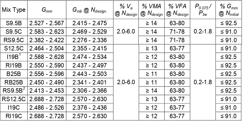
Table 3.5. Mix Verification Criteria for the Twelve Most Commonly used Mix Types in NC
Mix Type Gmm Gmb@ Ndesign.
% Va
@ Ndesign
% VMA
@ Ndesign
% VFA
@ Ndesign
P0.075 /
Pbe
% Gmm
@ Ninitial
S9.5B 2.527 - 2.567 2.415 - 2.475 ≥ 14 63-80 ≤ 92.5
S9.5C 2.583 - 2.623 2.469 - 2.529 ≥ 14 71-78 ≤ 91.0
RS9.5C 2.382 - 2.422 2.276 - 2.336
2.0-6.0
≥ 14 71-78
0.2-1.8
≤ 91.0
S12.5C 2.464 - 2.504 2.355 - 2.415 ≥ 13 63-77 ≤ 91.0
I19B1 2.588 - 2.628 2.474 - 2.534 ≥ 12 63-80 ≤ 92.5
RI19B 2.550 - 2.590 2.437 - 2.497 ≥ 12 63-80 ≤ 92.5
B25B 2.556 - 2.596 2.443 - 2.503 ≥ 11 63-80 ≤ 92.5
RB25B 2.450 - 2.490 2.341 - 2.401 ≥ 11 63-80 ≤ 92.5
RS9.5B2 2.413 - 2.453 2.306 - 2.366 ≥ 14 63-80 ≤ 92.5
RS12.5C 2.688 - 2.728 2.570 - 2.630 ≥ 13 63-77 ≤ 91.0
I19C 2.486 - 2.526 2.376 - 2.436 ≥ 12 63-77 ≤ 91.0
RI19C 2.688 - 2.728 2.570 - 2.630
2.0-6.0
≥ 12 63-77
0.2-1.8
≤ 91.0
1The mix design sheet for this mix shows a traffic level of “less than 0.3 million” ESALs. This number is a
mistake that has been corrected to become “less than 3 million”.
2This JMF replaces the one submitted to NCSU in an early stage of this research; the original JMF mix is no
13
The volumetrics for each mixture were determined and compared with the
corresponding criteria outlined in Table 3.5. Performance test specimens were fabricated for mixtures that satisfied the mixture verification criteria. A new mixture design was performed for mixtures that failed the mixture verification criteria shown in Table 3.5.
3.2.2 Wet Sieve Analysis
Aggregate stockpiles for all twelve mixes were analyzed for gradation following ASTM C136-06 test standards (ASTM, 2006). Table 3.6 compares the combined gradations determined from the wet sieve analysis (WSA) and the corresponding JMF numbers.
Table 3.6 Combined Aggregate Gradations Obtained from Wet Sieve Analysis vs. JMF
S9.5B RS9.5B S9.5C RS9.5C S12.5C RS12.5C
Sieve Size
WSA JMF WSA JMF WSA JMF WSA JMF WSA JMF WSA JMF
1" 100 100 100 100 100 100 100 100 100 100 100 100
3/4" 100 100 100 100 100 100 100 100 99 100 99 100
1/2" 100 100 100 100 100 100 100 100 99 100 99 100
3/8" 98 96 97 96 98 97 97 97 88 89 89 89
No.4 72 67 79 75 71 68 83 79 68 66 67 72
No.8 48 48 56 57 48 48 65 59 47 49 46 52
No.16 38 37 38 44 34 34 47 43 32 35 31 34
No.30 31 30 26 30 25 25 32 32 21 25 23 25
No.50 23 21 17 21 17 18 20 21 13 15 16 16
No.100 12 11 10 12 11 12 10 12 7 8 9 9
No.200 6 6 6 6 6 6 5 7 5 5 5 5
I19B RI19B I19C RI19C B25B RB25B
Sieve Size
WSA JMF WSA JMF WSA JMF WSA JMF WSA JMF WSA JMF
1" 100 100 100 100 100 100 100 100 100 99 99 98
3/4" 100 100 97 99 100 100 98 97 84 83 85 82
1/2" 100 100 80 84 100 100 87 85 68 69 72 71
3/8" 74 73 70 75 76 78 76 75 62 63 68 68
No.4 51 50 48 51 55 52 39 39 46 45 53 48
No.8 37 36 36 38 40 38 22 24 34 30 38 35
No.16 29 28 29 31 30 29 17 19 23 19 27 26
No.30 24 23 19 24 20 20 13 15 16 13 19 19
No.50 18 16 10 14 12 11 10 11 11 9 13 14
No.100 10 9 6 8 7 7 7 8 8 6 8 7
14
The data shown in Table 3.6 are a valuable part of the future material database, especially given that the twelve mixes had undergone different types of testing.
Table 3.7 summarizes the percentage of differences in combined stockpile gradations between the corresponding numbers in the JMF and those measured.
Table 3.7. Percentage Differences between JMF and Measured Combined Gradations
Mixture ID Sieve
Size S9.5B RS9.5B S9.5C RS9.5C S12.5C RS12.5C
1" 0 0 0 0 0 0
3/4" 0 0 0 0 -1 -1
1/2" 0 0 0 0 -1 -1
3/8" 2 1 1 0 -1 0
No.4 7 5 4 5 3 -7
No.8 0 -2 0 10 -4 -12
No.16 3 -14 0 9 -9 -9
No.30 3 -13 0 0 -16 -8
No.50 10 -19 -6 -5 -13 0
No.100 9 -17 -8 -17 -13 0
No.200 0 0 0 -29 0 0
Mixture ID Sieve
Size I19B RI19B I19C RI19C B25B RB25B
1" 0 0 0 0 1 1
3/4" 0 -2 0 1 1 4
1/2" 0 -5 0 2 -1 1
3/8" 1 -7 -3 1 -2 0
No.4 2 -6 6 0 2 10
No.8 3 -5 5 -8 13 9
No.16 4 -6 3 -11 21 4
No.30 4 -21 0 -13 23 0
No.50 13 -29 9 -9 22 -7
No.100 11 -25 0 -13 33 14
No.200 0 -20 0 0 25 25
15
percent and 29 percent. These differences could be attributed to changes in the crushing and handling equipment at the different quarries. Soft aggregate might be crushed such that it exhibits different gradations even though the same equipment is used. Differences also could be caused by reaching a different layer in the aggregate stockpile or the changes in the aggregate quarry.
These differences in the gradations between the JMF and actual stockpiles make it difficult to obtain the same target gradation in the JMF. That is, if the stockpile percentages in the JMF were used with the materials obtained for this research, the gradation of the blended aggregate would be different from the blended gradation in the JMF. It is noted that the goal of this laboratory experimental program is to produce mixtures that are as similar as possible to those that contractors would produce in the field using the same materials and JMFs. In actual construction, contractors would apply the stockpile percentages in the JMF to the materials they acquire for the paving job. Therefore, the same approach, i.e., using the stockpile percentages in the JMF, was chosen for this study.
3.2.3 Measurement of Aggregate Dry Bulk-Specific Gravity (Gsb)
With the scope of this research work in mind, the dry bulk-specific gravity (Gsb)
values from the JMF were used in calculating the volumetrics of the mixtures. Again, the goal is to simulate the expected outcome in the field when a contractor takes a current JMF and uses it with the available materials. Therefore, to best characterize all twelve
representative mixtures chosen for this project, the current JMF numbers were used with the currently available materials. As mentioned earlier, for mixtures that did not meet the criteria, a modification was made to the mixtures or a new mixture design was created prior to the fabrication of any performance specimens.
The measured Gsb values represent the correct bulk-specific gravity for the current
materials. Correct Gsb values are vital for two reasons:
16
• Second, they are used to check the effects of the differences in Gsb, i.e., between the
JMF numbers and the measured numbers, on the volumetrics of the mixtures.
Because of the imperative role that the bulk-specific gravity plays in mixture design and volumetrics, and because of the two reasons cited, the M&T Unit at the NCDOT was asked to measure the bulk-specific gravity of all the stockpiles for each of the twelve mixes. Aggregate stockpiles were sampled in the field following AASHTO T2 standards
(AASHTO-a) to obtain enough materials for all characterization testing. Samples were then reduced in size for bulk-specific gravity testing.
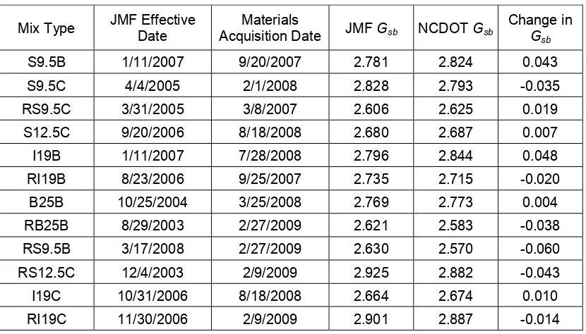
Table 3.8 summarizes the bulk-specific gravity test results as measured by the NCDOT and compares these results to the values reported in the JMF. Worth mentioning is that the M&T Unit measured only the bulk-specific gravity for the stockpiles; however, sieve analysis information, needed to calculate the combined aggregate specific gravities, was obtained at NCSU through a complete wet sieve analysis. In addition to bulk-specific gravity results, Table 3.8 also summarizes the JMF’s effective dates and the date the new aggregate materials were acquired.
Table 3.8. Change in Dry Bulk-Specific Gravity (Gsb) Over Time
Mix Type JMF Effective Date Acquisition Date Materials JMF Gsb NCDOT Gsb Change in G
sb
S9.5B 1/11/2007 9/20/2007 2.781 2.824 0.043
S9.5C 4/4/2005 2/1/2008 2.828 2.793 -0.035
RS9.5C 3/31/2005 3/8/2007 2.606 2.625 0.019
S12.5C 9/20/2006 8/18/2008 2.680 2.687 0.007
I19B 1/11/2007 7/28/2008 2.796 2.844 0.048
RI19B 8/23/2006 9/25/2007 2.735 2.715 -0.020
B25B 10/25/2004 3/25/2008 2.769 2.773 0.004
RB25B 8/29/2003 2/27/2009 2.621 2.583 -0.038
RS9.5B 3/17/2008 2/27/2009 2.630 2.570 -0.060
RS12.5C 12/4/2003 2/9/2009 2.925 2.882 -0.043
I19C 10/31/2006 8/18/2008 2.664 2.674 0.010
17
Table 3.9 summarizes the effects that changes in the bulk-specific gravity values have on mix volumetrics, i.e., the voids in mineral aggregates (VMA), voids filled with asphalt
(VFA), and the dust proportion (DP), defined as the ratio of dust divided by effective binder
content. The shaded fields in Table 3.9 correspond to volumetrics that did not satisfy the criteria presented in Table 3.5. Table 3.9 shows that out of the twelve mixtures, mixture I19B and mixture RS9.5B both failed the criteria. Therefore, these two mixtures need to be re-designed to meet the criteria in Table 3.5.
Table 3.9. Effect of the Change in Dry Bulk-Specific Gravity on HMA Mix Volumetrics
Volumetrics using JMF Gsb Volumetrics using NCDOT Gsb
Mix Type
VMA VFA Dust/Binder VMA VFA Dust/Binder
S9.5B 15.6 78.8 1.1 16.8 80.4 1
S9.5C 15.6 75.7 1.2 14.6 73.9 1.4
RS9.5C 16.5 77.6 1.3 17.1 78.4 1.2
S12.5C 16.2 73.2 0.9 16.4 73.6 0.9
I19B 13.6 81.9 1 15 83.6 0.9
RI19B 14.1 72.4 1.2 13.4 71 1.2
B25B 14.8 67.3 1 15 67.8 0.9
RB25B 13.7 67.9 1.1 12.4 64.6 1.2
RS9.5B 17.9 65.3 1.1 16 61.2 1.3
RS12.5C 15.8 69 1.1 14.6 66.3 1.2
I19C 14.1 69.1 1.2 14.4 69.8 1.2
RI19C 14.9 68.3 1.2 14.5 67.4 1.3
3.2.4 Reclaimed Asphalt Pavement (RAP) Materials
18
exists between the RAP asphalt content measured in the lab and that reported in the JMF, with the exception of the RAP component of the RB25B mixture, which suggests a decrease in the amount of binder of about 1.2 percent.
Table 3.10. Summary of Asphalt Binder Content for HMA Mixes with RAP
Mix Type % AC - Manual Weighing Machine % AC - Average % AC - % AC Reported in JMF
RS9.5B 5.59 5.58 5.6 5.6
RS9.5C 5.28 5.22 5.3 5.2
RS12.5C 4.40 4.33 4.4 4.5
RI19B 4.45 4.80 4.6 4.6
RI19.0C 4.52 4.55 4.5 4.5
RB25.0B 4.34 4.31 4.3 5.5
3.2.5 Mixture Verification Results
One-point mixture verification tests were performed for each of the twelve mixtures prior to fabricating any performance test specimens. New materials were batched according to the JMF stockpile gradations and percentages in an attempt to simulate mixtures that would be produced in the field if similar JMF were used. Table 3.11 summarizes the one-point verification test results by showing all measured and calculated mixture volumetrics. The shaded fields in Table 3.11 correspond to the parameters that failed the criteria presented in Table 3.5.
Table 3.11 shows that three of the twelve mixtures failed the criteria for one
component or another. The mixtures that failed are S9.5B, I19.0B, and RS9.5B. The I19.0B and RS9.5B mixtures have failed the criteria in Table 3.9. Using the same aggregate
19
Table 3.11. One-Point Mix Verification Test Results
Mix Type Gmm Gmb@
Ndesign
% Va
@ Ndesign
% VMA
@ Ndesign
% VFA
@ Ndesign
P0.075/Pbe % @ Gmm
Ninitial
S9.5B 2.587 2.501 3.3 15.6 78.8 1.1 90.3
S9.5C 2.616 2.517 3.8 15.6 75.7 1.2 87.8
RS9.5C 2.414 2.324 3.7 16.5 77.6 1.3 89.6
S12.5C 2.495 2.376 4.3 16.2 73.2 0.9 89.3
I19B 2.633 2.544 2.5 13.6 81.9 1.0 91.2
RI19B 2.558 2.458 3.9 14.1 72.4 1.2 90.1
B25B 2.593 2.467 4.8 14.8 67.3 1.0 86.5
RB25.0B 2.472 2.361 4.4 13.7 67.9 1.1 88.7
RS9.5B 2.417 2.282 6.2 17.9 65.3 1.1 87.1
RS12.5C 2.712 2.575 4.9 15.8 69 1.1 88.1
I19C 2.519 2.397 4.3 14.1 69.1 1.2 89.5
RI19.0C 2.722 2.58 4.7 14.9 68.3 1.2 85.3
Table 3.12. Four-Point Mix Design Test Results and Recommended Asphalt Contents
Mix Type New % AC Gmm
Gmb @
Ndesign
% Va
@ Ndesign
% VMA
@ Ndesign
% VFA
@ Ndesign P0.075/Pbe %
Gmm
@ Ninitial
S9.5B 5.9 2.574 2.501 4 15.4 74 1.1 90.3
I19B 4.8 2.641 2.534 4 13.7 71 1.1 89.9
RS9.5B 6 2.397 2.3 4 17.8 77 0.9 88.9
After the mixture design verification process was completed successfully for all twelve mixtures, a target air content was determined for the performance test specimens. Section 3.3 presents the process for determining this target air content.
3.3 Selection of a Target Air Void Percentage for Performance Test Specimens
The process of selecting the proper target air void percentage for performance
specimens has two important dimensions. First, the effective calibration and validation of the distress prediction models employed by the MEPDG require the air void percentage at the time of construction (also referred to as as-constructed or original air voids). Second, the air
20
layers in future construction, because the performance model coefficients to be determined from this study will form the basis for the Level 2 database for future use in the MEPDG.
In order to have a consistent target air content that can be used with all mixtures throughout this project, a literature review was carried out to search for national field mixture densification data that could help in identifying an air void level that is both representative of the initial stage after construction and that also promises successful specimen fabrication in the laboratory.
In the NCHRP 9-9 project, Superpave Mix Design: Verifying Gyration Level in the Ndesign Table, Prowell and Brown (2007) attempted to verify the Ndesign levels in the field.
Samples were collected from 40 field projects at the time of construction. These field projects were located in 16 states and represent a wide range of traffic levels, asphalt binder grades, aggregate types, and gradations. The final report (NCHRP 573) contains a table that presents the changes in the percentage of the maximum specific gravity, Gmm, over time.
Table 3.13 summarizes the average changes in air void levels over two years using the data collected from all 16 states. Table 3.14 is a modification of the table documented in NCHRP 573 and presents the changes in air void levels over time instead of the changes in percentage of Gmm. The shaded fields in Table 3.14 correspond to data anomalies, which
were ignored when calculating the averages reported in Table 3.13.
Table 3.13. Changes in Air Void Levels over Time – Results from 16 States
Time Construction 3 months 6 months 1 year 2 years
% Air Voids 8.3 6.3 6.2 5.6 5.2
21
Table 3.14. Project NCHRP 9-9 Average In-Place Air Voids
Average Percentage of Air Voids
Project ID Roadway
Construction 3 months 6 months 1 year 2 years
AL-1 Hwy 157 11.3 6.8 6.4 7.0 6.1
AL-2 Hwy 168 11.7 9.7 9.8 9.8 8.2
AL-3 Hwy 80 10.3 7.2 6.8 6.7 6.4
AL-4 Hwy 84 11.6 7.2 6.9 7.4 5.7
AL-5 Hwy 167 10.3 6.4 6.2 6.9 5.4
AL-6 Andrews Rd. 8.2 6.9 7.3 6.9 6.7
AR-1 I-40 8.0 6.9 6.5 5.9 5.8
AR-2 I-55 10.6 9.1 8.6 8.2 8.2
AR-3 I-40 8.5 5.4 5.2 5.2 5.3
AR-4 I-30 9.1 5.8 6.5 5.5 5.5
CO-1 Hwy 9 6.2 3.1 3.5 2.8 1.9
CO-2 Hwy 82 5.3 3.4 3.4 3.1 2.9
CO-3 I-70 6.5 5.4 4.0 4.4 4.3
CO-4 Hwy 13 6.3 6.7 7.2 5.8 5.8
CO-5 Hwy 82 8.4 6.4 6.3 5.8 6.2
FL-1 Davis Hwy 8.2 5.8 5.2 5.7 4.8
GA-1 Buford Hwy 5.0 4.3 4.2 4.0 3.5
IL-1 I-57 9.0 6.1 6.2 5.8 5.6
IL-2 I-64 8.2 5.8 5.9 5.6 4.8
IL-3 I-70 7.8 5.7 6.1 5.6 5.5
IN-1 US 136 8.7 9.7 9.7 37.7 6.5
IN-2 I-69 8.6 9.3 8.3 5.3 5.9
KS-1 I-70 10.1 8.8 7.9 6.4 6.4
KY-1 CR 1796 14.5 12.7 13.3 12.3 11.5
KY-2 I-64 7.8 6.8 6.7 6.1 5.9
KY-3 CR 1779 7.4 6.9 6.3 5.7 5.8
MI-1 I-75 8.7 7.9 7.2 6.6 5.2
MI-2 Hwy 50 6.9 4.8 3.9 3.2 3.2
MI-3 Hwy 52 7.0 6.3 5.5 N/A 3.5
MO-1 I-70 6.6 3.6 4.4 4.2 3.5
MO-2 Hwy 65 7.4 5.8 7.3 5.6 4.9
MO-3 I-44 6.5 5.6 5.7 4.7 4.4
NC-1 I-85 9.9 7.2 8.3 7.0 6.6
NE-1 Hwy 8 7.4 4.6 4.5 4.7 4.3
NE-2 Hwy 77 7.0 4.8 5.0 4.7 4.3
NE-3 Hyw 8 9.0 5.2 4.9 5.0 4.6
NE-4 I-80 7.8 5.1 4.8 3.3 2.8
TN-1 Hwy 171 8.9 6.9 6.9 5.9 5.7
UT-1 Hwy 150 8.1 6.5 6.8 N/A 6.3
22
CHAPTER 4 UNBOUND MATERIALS CHARACTERIZATION
4.1 Introduction
The scope of this research work includes the characterization of asphalt concrete materials for rutting and fatigue distresses that occur in flexible pavements. Unbound base and subgrade layers have not been characterized as part of this dissertation work. However, a GIS-based methodology has been developed to take advantage of the product of the NCHRP 9-23A project to determine subgrade soil properties for any location in North Carolina. Details regarding this methodology are presented in the following Section 4.2. For unbound base materials, the author recommends that a separate project should be funded to
characterize the most commonly used unbound base and sub-base materials in North
Carolina. In the meantime, the author recommends that the MEPDG default values should be used for unbound base and sub-base materials.
4.2 GIS-Based Implementation Methodology for the NCHRP 9-23A Recommended Soil Parameters for Use as Input to the MEPDG
4.2.1 Introduction