Dr. Marie Davidian.)
by
Chia-Cheng Chen
A dissertation submitted to the Graduate Faculty of North Carolina State University
in partial fullfillment of the requirements for the Degree of
Doctor of Philosophy
Statistics
Raleigh, North Carolina
2009
APPROVED BY:
Dr. Anastasios A. Tsiatis Dr. Huixia Wang
Dr. Huiman X. Barnhart Dr. Marie Davidian
To
My Parents
and
BIOGRAPHY
I would like to express my deepest appreciation to my advisors, Dr. Huiman X. Barnhart and Dr. Marie Davidian. Without their guidance, support, and patient throughout my dissertation work, it will be very difficult for me to obtain my Ph.D. degree. Dr. Huiman X. Barnhart especially directed my research work to the area of assessing reliability and agreement. I not only learned a lot from doing research in this field, but also realized how to express my thinking more efficiently and accurately, and how to do an independent research. I also appreciate my committee members, Dr. Anastasios A. Tsiatis and Dr. Huixia Wang, for their suggestions and teaching during my graduate days at NC State. I appreciate the chance and environment that the Statistics department offers to me for my graduate study at NC State.
TABLE OF CONTENTS
LIST OF TABLES . . . vii
LIST OF FIGURES . . . x
1 Comparison of ICC and CCC for assessing agreement for data without and with replications . . . 1
1.1 Introduction . . . 1
1.2 Comparisons of ICC and CCC . . . 3
1.2.1 Definitions and estimates ofICCsand CCC . . . 4
1.2.2 Comparisons ofE(ICC) andd CCC under the general model . . . . 7
1.3 Examples . . . 10
1.4 Discussion . . . 19
2 The random-observers concordance correlation coefficient . . . 20
2.1 Introduction . . . 20
2.2 Methodology . . . 22
2.2.1 CCCinter R for inter-observer agreement . . . 22
2.2.2 CCCintra R for intra-observer agreement . . . 24
2.2.3 CCCRabs for absolute agreement . . . 25
2.3 Estimation and Inference . . . 26
2.4 Simulations . . . 28
2.5 Examples . . . 34
2.5.1 Vertebral Body Data . . . 34
2.5.2 Image Data . . . 41
3 Assessing agreement with intraclass correlation coefficient and concor-dance correlation coefficient with repeated measures . . . 50
3.1 Introduction . . . 50
3.2 Methodology . . . 51
3.2.1 CCC for random observers and fixed times . . . 57
3.2.2 CCC for fixed observers and random times . . . 60
3.2.3 CCC for fixed observers and fixed times . . . 63
3.2.4 ICC for repeated measurements . . . 66
3.3 Estimation and Inference . . . 71
3.3.1 Estimation and Inference forCCC . . . 71
3.3.2 Estimation and Inference forICC . . . 77
3.4 Data Analysis . . . 80
3.5 Discussion . . . 83
LIST OF TABLES
Table 1.1 The ANOVA table forICCs for blood pressure data by number of replicates 16
Table 1.2 Estimates of the ICCs and CCCs for blood pressure data by number of replicates . . . 16
Table 1.3 Estimates of individual parameters for blood pressure data by number of replicates . . . 16
Table 1.4 The ANOVA table for ICCs for PEFR data by number of replicates . . . 18
Table 1.5 Estimates of the ICCsand CCCs for PEFR data by number of replicates . 18
Table 1.6 Estimates of individual parameters for PEFR data by number of replicates 18
Table 2.1 Three scenarios of the true values for the proposedCCCR. . . 30
Table 2.2 Results of CCCabs
R based on 1000 Monte Carlo data sets . . . 31
Table 2.3 Results of CCCinter
R based on 1000 Monte Carlo data sets . . . 32
Table 2.4 Results of CCCintra
R based on 1000 Monte Carlo data sets . . . 33
Table 2.5 Description statistics for readings between times by readers and locations in Situation 1 for vertebral body data . . . 37
Table 2.8 Results of the estimates and improved 95% bootstrap-t confidence intervals ofCCCR and the estimates ofρc,rm for two situations for vertebral body data . . . . 40
Table 2.9 Description statistics for readings between times by readers and variables for image data . . . 48
Table 2.10 Description statistics for readings between readers by times and variables for image data . . . 48
Table 2.11 Description statistics for readings between readers and times by variables for image data . . . 49
Table 2.12 Results of the estimates and improved 95% bootstrap-t confidence intervals ofCCCR and the estimates ofρc,rm for image data . . . 49
Table 3.1 Existing methods (Yes, No) for four cases comparing observer with repeated measures under different approaches and indices . . . 52
Table 3.2 Definitions and results ofCCC for inter-observer, intra-observer, and absolute agreement under four cases . . . 54
Table 3.3 Definitions ofICC for inter-observer, intra-observer, and absolute agreement under four cases based on the corresponding ANOVA modelsa. . . 56
Table 3.4 Mean square expecations for three-way ANOVA models based on Yijk =
µ+µPi +µTk +µOj +µP Tik +µP Oij +µT Okj +eP OTijk ,whereP,O, andT are random . . . 78
Table 3.5 Mean square expecations for three-way ANOVA models based on Yijk =
µ+µP
i +µtk+µOj +µP tik +µijP O+µtOkj +eijkP OT,whereP,O are random andtis fixed 79
Table 3.6 Mean square expecations for three-way ANOVA models based on Yijk =
µ+µP
Table 3.7 Mean square expecations for three-way ANOVA models based on Yijk =
µ+µP
i +µtk+µoj+µP tik +µijP o+µtokj+eP otijk,where P is random, and o,tare fixed. 79
Table 3.8 Results of the estimates and improved 95% bootstrap-t confidence intervals ofCCC under four cases for image data . . . 81
LIST OF FIGURES
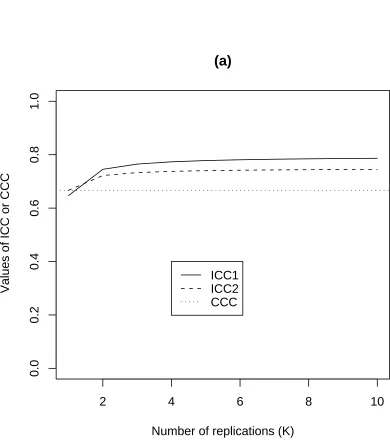
Figure 1.1 Plots of ICC and CCC values as function ofK with ρµ12 = 0.8 . . . 11
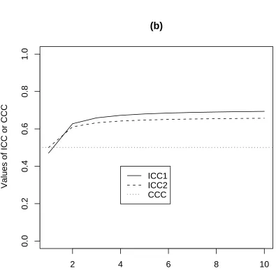
Figure 1.2 Plots of ICC and CCC values as function ofK with ρµ12 = 0.6 . . . 12
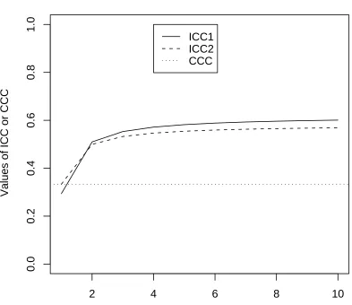
Figure 1.3 Plots of ICC and CCC values as function ofK with ρµ12 = 0.4 . . . 13
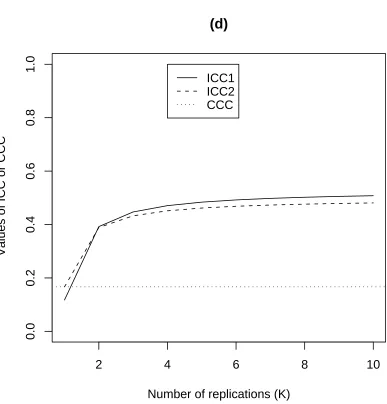
Figure 1.4 Plots of ICC and CCC values as function ofK with ρµ12 = 0.2 . . . 14
Figure 2.1 Scatter plots between readers for the Anterior at the first time point in Situation 1 for vertebral body data . . . 42
Figure 2.2 Scatter plots between readers for the Anterior at the second time point in Situation 1 for vertebral body data . . . 43
Figure 2.3 Scatter plots between readers for the Posterior at the first time point in Situation 1 for vertebral body data . . . 44
Figure 2.4 Scatter plots between readers for the Posterior at the second time point in Situation 1 . . . 45
Figure 2.5 Scatter plots between readers of all T locations in Situation 2 for vertebral body data . . . 46
Chapter 1
Comparison of ICC and CCC for
assessing agreement for data
without and with replications
1.1
Introduction
correlation coefficient (ICC) and the concordance correlation coefficient (CCC), that may take the systematic shifts into account in assessing agreement.
The intraclass correlation coefficient (Fisher, 1925) originated from genetics and was first applied to social science and then to medical science thereafter to assess agreement or reliability between observers. We focus on ICCs for assessing agreement between ob-servers where there are only subject and observer effects in the models. Extensions ofICC for data with other factors, such as repeated measures, have been proposed by Vangeneug-den et al. (2005) and are not considered in this chapter. The original ICC was based on the one-way ANOVA model. Extensions of this ICC lead to other versions of ICCsbased on the two-way ANOVA models (Bartko, 1966). Because different versions of ICCs can give different results depending on the chosen ANOVA models (Bartko, 1966; Shrout and Fleiss, 1979; M¨uller and B¨uttner, 1994; McGraw and Wong, 1996), M¨uller and B¨uttner (1994) proposed simple rules to choose a suitableICC with respect to the underlying data setting. However, researchers may compute theseICCswithout verifying the assumptions and theICC is biased if the ANOVA assumptions are not met. Therefore, there is a need to get a sense of the population parameter that the ICC estimator provides under a general setting.
multiple observers with replicated measurements under the two-way ANOVA model with-out interaction, which is a special case of CCC by Barnhart et al. (2005) for data with replication.
If the ANOVA assumptions are met, the CCC usually reduces to theICC defined by the ANOVA model (Barnhart et al. 2002). However, it is not clear what the ICC estimates are estimating if the ANOVA model does not hold. For data without replications, there were some comparisons of CCC and ICC when the ANOVA model does not hold (McGraw and Wong, 1996; Nickerson, 1997; Carrasco and Jover, 2003). For example, Nickerson showed that the estimates for the ICCs (ICC2 andICC3 defined here in Section 1.2.1) defined by two-way ANOVA models are similar to the estimate for theCCC. Carrasco and Jover (2003) showed that the CCC corresponds mathematically to theICC (ICC2 in Section 1.2.1) defined by two-way ANOVA model without interaction even if the ANOVA assumptions are not met.
In this paper, we provide systematic and in-depth comparisons of three types of ICC with CCC for both data with and without replications. This includes reproducing the results shown by Nickerson (1997) and Carrasco and Jover (2003). In Section 1.2, we describe the notations used to summarize different versions of ICCs as in Barnhart et al. (2007) into three types ofICCsused for assessing agreement. The ANOVA models that de-fine the types ofICCsand the corresponding moment estimates for data with and without replication are presented. The CCC is also presented for data with and without replica-tion under the general model. We then compute the expectareplica-tions of the ICC estimators under the general model and compare them to the CCC defined by the general model. A blood pressure example and a peak expiratory flow rate example are used to illustrate the comparisons of the ICCs and the CCC for data with different number of replications in Section 1.3. Finally, Section 1.4 concludes with some discussions.
1.2
Comparisons of ICC and CCC
observers is treated as reference.
Following Barnhart et al. (2007), we use unified notations to summarize these existing versions of ICCs in three types under three kinds of ANOVA models for both cases of random and fixed observers. We note that one version of ICC, ICC3c (shown
below), is not used for comparison with the CCC because it is a measure of consistency rather than agreement. We present the definitions of the threeICCsand theCCC for data without replication (K= 1) and with replications (K >1) together. However, comparisons of ICC estimators with CCC is presented separately for data without replication (K= 1) and with replications (K >1) in Section 1.2.2. The definitions of three types of ICC and CCC are presented below. Following the existing literature, the corresponding estimates for ICCs are obtained through the method of moments based on the expectation of the mean sums of squares from the ANOVA models.
1.2.1 Definitions and estimates of I CCs and CCC
Let Yijk be thekth replicated reading for observerj on the subjecti,i= 1, ..., N,
j = 1, ..., J, k= 1, ..., K. The first and original ICC,ICC1, is defined under the one-way ANOVA model given by
Yijk =µ+αi+eijk,
where µ is the overall effect common to all methods, αi is the random effect of subject i,
which is independent and identically distributed (i.i.d.) with normal distributionN(0, σα2), and eijk is the random error, which is i.i.d. with normal distribution N(0, σ2e); αi and
eijk are mutually independent. The ICC1 and the corresponding estimator (Bartko, 1966;
Shrout and Fleiss, 1979; McGraw and Wong, 1996) are
ICC1 = σ2α σ2
α+σe2
, ICC\1 =
M Sα−M Se
M Sα+ (JK−1)M Se
,
whereM Sα = NJ K−1PNi=1( ¯Yi..−Y¯...)2 andM Se= (J K−11)N PNi=1 PJ
j=1 PK
k=1(Yijk−Y¯i..)2 are
the means of the sums of squares from the one-way ANOVA model for between and within subjects, respectively. ¯Yi.. =PJj=1
PK
k=1Yijk/(JK), ¯Y... = PNi=1 PJ
j=1
PK
IfK = 1,
\
ICC1 = M Sα−M Se M Sα+ (J−1)M Se
.
The second and third ICCsare based on two-way ANOVA model without inter-action and with interinter-action, respectively. The two-way ANOVA model without interinter-action is given by
Yijk =µ+αi+βj+eijk,
where µ, αi, and eijk are as before. If observers are treated as random, then βj is the
random effect of observer j, which is i.i.d. with normal distribution N(0, σ2β) and αi, βj,
and eijk are mutually independent. If observers are treated as fixed, we use notation
σβ2 = PJj=1β2j/(J −1) with constraint PJj=1βj = 0. Then ICC2 and the
correspond-ing estimator (McGraw and Wong, 1996) are
ICC2 =
σ2α σ2
α+σβ2+σe2
, ICC\2 =
M Sα−M Se
M Sα+ (JK−1)M Se+J(M Sβ−M Se)/N
,
where M Sα = NJ K−1PNi=1( ¯Yi..−Y¯...)2, M Se = (J K−1)1N−J+1PNi=1 PJ
j=1
PK
k=1(Yijk−Y¯i..−
¯
Y.j.+ ¯Y...)2, and M Sβ = JN K−1PJj=1( ¯Y.j.−Y¯...)2.If K= 1,
\
ICC2 =
M Sα−M Se
M Sα+ (J−1)M Se+J(M Sβ−M Se)/N
.
Considering the interaction between observer and subject, the two-way ANOVA model with interaction is given by
Yijk=µ+αi+βj+γij +eijk,
where µ, αi, βj, and eijk are as before; γij is the random effect of the observer-subject
interaction, which isi.i.d.withN(0, σγ2);αi,βj,γij, andeijk are mutually independent ifβj
is random. Ifβj is fixed, notationσ2β =PJj=1β2j/(J−1) is used with constraints
Fleiss, 1979; McGraw and Wong, 1996) are
ICC3 =
σ2
α
σ2
α+σβ2+σγ2+σe2
(random βj), ICC3 =
σ2α−σγ2/(J−1) σ2
α+σ2β+σγ2+σ2e
(f ixed βj),
\
ICC3 = M Sα−M Sγ
M Sα+J(K−1)M Se+ (J−1)M Sγ+J(M Sβ−M Sγ)/N
,
where M Sα = NJ K−1PNi=1( ¯Yi.. − Y¯...)2, M Se = N J(K1−1)PNi=1PJj=1PKk=1(Yijk − Y¯ij.)2,
M Sβ = JN K−1PJj=1( ¯Y.j.−Y¯...)2, and M Sγ = (J−1)(KN−1)PNi=1PJj=1( ¯Yij.−Y¯i..−Y¯.j.+ ¯Y...)2.
IfK = 1,M Sγ is simply nonestimable and therefore is included inM Se, thus
\
ICC3 =
M Sα−M Se
M Sα+ (J−1)M Se+J(M Sβ−M Se)/N
=ICC\2.
Note that in the case where observers are treated as fixed effect to have a two-way mixed effect model, Bartko (1966) (and later corrected by Bartko (1974) and Shrout and Fleiss (1979)) defined the following version of ICC based on correlation:
ICC3c =
σ2
α−σ2γ/(J−1)
σ2
α+σγ2+σe2
,
McGraw and Wong (1996) called thisICC as theICC for consistency since the systematic deviation due to method, σβ2, is not included in the denominator. Because this ICC is a measure for consistency andCCC is a measure of agreement, we do not compareICC3c to
CCC in this paper.
We present the CCC below for assessing agreement betweenJ observers for data with K replications (K = 1 or K > 1) under the general model, Yijk =µij +eijk
(Barn-hart et al., 2005). We use the following minimal assumptions if the K readings measured by the same observer on a subject are true replications. (1) µij and eijk are independent
with means of E(µij) =µj and E(eijk) = 0; (2) between-subject and within-subject
vari-ances are V ar(µij) = σ2Bj and V ar(eijk) = σW j2 , respectively; (3) Corr(µij, µij′) = ρµjj′,
denotes the total variability of observerj, andρjj′ =Corr(Yijk, Yij′k′) denotes the pairwise
correlation between two readings from observers j andj′. The CCC is defined as
ρc = 1−
PJ−1
j=1
PJ
j′=j+1E(Yijk−Yij′k′)2
PJ−1
j=1 PJ
j′=j+1EI(Yijk−Yij′k′)2
= 2
PJ−1
j=1
PJ
j′=j+1σjσj′ρjj′
(J −1)PJj=1σ2j +PjJ=1−1PJj′=j+1(µj−µj′)2
=
1
J−1 PJ
j=1
PJ
j′=1(j′6=j)σBjσBj′ρµjj′
PJ
j=1σBj2 +
PJ
j=1σW j2 + (
PJ
j=1µ2j−J−11 PJ
j=1 PJ
j=1(j′6=j)µjµj′)
,
where EI is the expectation under independence of Yijk, Yij′k′. This CCC was referred
to as a fixed marginal agreement coefficient (FMAC) by Fay (2005). Fay also proposed a random marginal agreement coefficient (RMAC) if the EI(Yijk−Yij′k′)2 in the
denomina-tor is replaced by EZjEZj′(Zj −Zj′)
2, where Z
j and Zj′ are independent and identically
distributed random variables with a mixture distribution of 0.5Yj + 0.5Yj′. This RMAC is
closely related to E(ICC[1) as shown in Section 1.2.2.
For the special case whenJ=2 andK=1 (without replication), theCCC is reduced to the following originalCCC by Lin (1989).
ρc = 1−
E(Yi11−Yi21)2
E((Yi11−Yi21)2|corr(Yi11, Yi21) = 0)
= 2σB1σB2ρµ12
σB21+σ2W1+σ2B2+σW2 2+ (µ1−µ2)2
= 2σ1σ2ρ12 σ2
1+σ22+ (µ1−µ2)2
withρ12=Corr(Yi11, Yi21).Note here that theICCsare defined for both random and fixed
cases where the observers are treated as, while CCC is usually defined for fixed observers.
1.2.2 Comparisons of E(I CCd) and CCC under the general model
[
ICC defined in Section 1.2.1 under this general model. The expectations are presented for data without and with replications. Please note below that even E(ICC3) =\ CCC for all K, one may still have ICC\3 ≥CCC\ as indicated by Nickerson (1997) and Carrasco and Jover (2003). This is because that ( ¯Y.j. −Y¯.j′.)2 is usually used (Lin, 1989) to estimate
(µj −µj′)2 in\CCC. However, ( ¯Y.j.−Y¯.j′.)2 is a biased estimator of (µj−µj′)2 as pointed
out by Carrasco and Jover (2003). In general, the bias is small for moderate and large sample size. If this bias is corrected, then we haveICC\3 =\CCC as indicated by Nickerson (1997) for the case ofK = 1.
For data without replication, it can be shown that E(ICC1)\ ≈ E(M Sα−M Se)
E(M Sα+ (J −1)M Se)
= ( 1
J−1) PJ
j=1
PJ
j′=1(j′6=j)σBjσBj′ρµjj′−J1
−1( PJ
j=1µ2j −J1(
PJ
j=1µj)2)
PJ
j=1σBj2 +
PJ
j=1σW j2 +
PJ
j=1µ2j −J1(
PJ j=1µj)2
6
= CCC. Similarly,
E(ICC\2) ≈
E(M Sα−M Se)
E(M Sα+ (J −1)M Se+J(M Sβ−M Se)/N)
= (
1
J−1) PJ
j=1
PJ
j′=1(j′6=j)σBjσBj′ρµjj′
PJ
j=1σBj2 +
PJ
j=1σW j2 + (
PJ
j=1µ2j −J−11 PJ
j=1
PJ
j′=1(j′6=j)µjµj′)
= CCC
Because ICC\3 =ICC\2 when K = 1, thus, E(ICC\3) = E(ICC\2) =CCC. For the special case with J = 2 (two observers), we have
E(ICC\1) ≈
E(M Sα−M Se)
E(M Sα+M Se)
= 2σ1σ2ρ12− 1
2(µ1−µ2)2 σ2
1+σ22+12(µ1−µ2)2
6
It is interesting to note that thisE(ICC\1) based on the one-way ANOVA model is equivalent to the RMAC by Fay (2005) when there are two observers and no replication. We think that this is because the scaling termEZ1EZ2(Z1−Z2)
2 in the denominator of Fay’s RMAC equals to two times the total variability used inICC1 based on the one way ANOVA model. The fact thatZ1 andZ2arei.i.d.with a distribution of 0.5Y1+ 0.5Y2 is similar to assuming that there is no observer effect in the one way ANOVA model. In addition, the natural generalization of RMAC to define RMAC for the case of J > 2 and K > 1 is to replace the term EI(Yijk−Yij′k)2 in the definition of CCC by EZjEZ
j′(Zj−Zj′)
2. Because Fay’s RMAC is equivalent to ICC1 forJ = 2 and K = 1, we believe that the generalizations of Fay’s RMAC will be the same as ICC1 with one-way ANOVA model based on the above observation.
For the other two ICCs withJ = 2, we have, E(ICC\2) = E(ICC\3)
≈ E(M Sα−M Se)
E(M Sα+M Se+ 2(M Sβ−M Se)/N)
= 2σ1σ2ρ12
σ2
1 +σ22+ (µ1−µ2)2 = CCC.
This confirms the same findings shown by Nickerson (1997) and Carrasco and Jover (2003) for data without replications.
For data with replications, the expressions for the expected values ofICC\1,ICC\2, and ICC\3 under the general modelYijk =µij +eijk are presented in the Appendix due to
may be a loss of efficiency of using ICC3 in relation toICC2 because extra parameters are estimated in ICC3.
To better understand the dependency of ICC1 andICC2 on the number of repli-cations, we consider a special case of J = 2 where the between-subject variances of two observers are the same (σB21 = σB22 = σB2), and the within-subject variances of two ob-servers are the same (σW2 1 =σW2 2 =σW2 ), especially when K is large and goes to infinity, then
lim
K→∞E(ICC\1) ≈
(1 +ρµ12)σB2
2σB2 + 2σ2W +12(µ1−µ2)2
≥ CCC, and
lim
K→∞E(\ICC2) ≈
(1 +ρµ12)σB2
(2 + N1 −N1ρµ12)σB2 + 2σ2W + (µ1−µ2)2
≥ CCC.
In this special case, limK→∞E(ICC\1) = CCC only if µ1 = µ2, and limK→∞E(ICC\2) = CCC only if ρµ12= 1.
To illustrate the dependency ofE(ICC\1) andE(ICC\2) on the number of replica-tions, we plotE(ICC1), E(\ ICC2),\ and CCC verses K in Figures 1.1-1.4. In these figures, we mimic the BP data in the Example Section by setting N = 85, σ2
B1 =σ2B2 = 955, and σ2
W1 =σW2 2 = 63. In addition, we setµ1 = 128 andµ2= 144. Figures 1.1-1.4 display plots of ICC and CCC values as function of K withρµ12 = 0.8, 0.6, 0.4, and 0.2, respectively. The value of CCC is ploted as a horizontal line because it does not depend on K.
From these figures, we see that E(ICC\1) is less than both of E(ICC\2) andCCC when K = 1 and increases quickly to the limit when K → ∞, which exceeds both of E(ICC2\) andCCC. E(ICC2) equals\ CCC whenK = 1 and increases quickly to the limit whenK→ ∞, which also exceedsCCC. For this special case, bothE(ICC\1) andE(ICC\2) are increasing functions ofK.
1.3
Examples
2
4
6
8
10
0.0
0.2
0.4
0.6
0.8
1.0
(a)
Number of replications (K)
Values of ICC or CCC
ICC1
ICC2
CCC
2
4
6
8
10
0.0
0.2
0.4
0.6
0.8
1.0
(b)
Number of replications (K)
Values of ICC or CCC
ICC1
ICC2
CCC
2
4
6
8
10
0.0
0.2
0.4
0.6
0.8
1.0
(c)
Number of replications (K)
Values of ICC or CCC
ICC1
ICC2
CCC
2
4
6
8
10
0.0
0.2
0.4
0.6
0.8
1.0
(d)
Number of replications (K)
Values of ICC or CCC
ICC1
ICC2
CCC
an automatic machine made three quick successive observations on 85 subjects’ (N=85) systolic blood pressure. For illustration, we compute estimates of three ICCs and CCC to assess agreement between the first observer and the automatic machine (J=2) for three scenarios:
(1) K=1 where only the first replication is used. (2) K=2 where only the first two replications are used. (3) K=3 where all three replications are used.
Table 1.1 shows the means of the sums of squares from the one-way ANOVA model, two-way ANOVA model without interaction, and two-way ANOVA model with interaction for different replications. The point estimations ofICCsand CCCs are shown in Table 1.2, where \CCCa and CCC\b are the estimates of CCC without and with bias corrections for estimating (µ1−µ2)2, respectively. Without the bias correction for estimating (µ1−µ2)2 inCCC\, theICC[
a
may be slightly larger than \CCC and even theoretically we have E(ICC) =[ E(\CCC). We summarize all the estimates of the parameters used in the definition of CCC by number of replications in Table 1.3. Please note that when K = 1, parameters ρµ12, σ2B1, σ
2
B2, σ
2
W1, and σ 2
W2 are nonestimable for data without replications. The ICC\1 is less than \CCC
a
when K = 1 and is greater than CCC\a when K > 1. The
\
ICC2 is close to and greater than\CCC
a
whenK = 1 but it is less thanICC\1whenK >1. As expected, ICC\2 = ICC\3 that is close to and greater than \CCC
a
and equivalent to
\
Table 1.1: The ANOVA table for ICCs for blood pressure data by number of replicates
ANOVA forICC1 ANOVA forICC2 ANOVA forICC3
Replicates M Sα M Se M Sα M Sβ M Se M Sα M Sβ M Sγ M Se
K = 1 1922.24 322.78 1922.24 11283.78 192.30 1922.24 11283.68 192.30 0
K = 2 3688.00 249.10 3688.00 21409.42 165.79 3688.00 21409.42 375.69 62.08
K = 3 5337.80 227.63 5337.80 31106.45 154.87 5337.80 31106.45 537.74 60.27
Table 1.2: Estimates of the ICCs and CCCs for blood pressure data by number of replicates
[
ICC1 ICC[2 ICC[3 \CCC
a
\
CCCb
K=1 .712 .728 .728 .727 .728
K=2 .775 .752 .707 .706 .708
K=3 .789 .758 .702 .701 .702
a
Moment estimator ofCCC without a bias adjustment
b
With adjustment of a bias correction term for estimating (µ1−µ2)2
Table 1.3: Estimates of individual parameters for blood pressure data by number of replicates
ˆ
ρ12 ρˆµ12 µˆ1 µˆ2 σˆB21 σˆ
2
B2 ˆσ
2
W1 σˆ
2
W2
K=1 .82 - 128.54 144.84 - - -
-K=2 .79 .84 127.92 143.79 957.30 1012.47 35.36 88.79
As a second example, we used the data of peak expiratory flow rate (PEFR) from Bland and Altman (1986). In this data set, two replications (K = 2) were made by each of the two methods (J = 2) for each of the 17 subjects (N = 17). The two methods are Wright peak flow meter and mini Wright meter. Similar to the first example, we compute estimates of threeICCs andCCC to assess agreement between the Wright peak flow meter and the mini Wright meter (J=2) for two scenarios when (1) K=1 where only the first replication is used and (2) K=2 where two replications are used.
Table 1.4 shows the means of the sums of squares from the one-way ANOVA model, two-way ANOVA model without interaction, and two-way ANOVA model with interaction for different replications. The point estimations of ICCs and CCC are shown in Table 1.5, where CCC\a and \CCCb are estimates ofCCC without and with bias corrections for estimating (µ1−µ2)2, respectively. As in the first example, we summarize all the estimates of the parameters used in the definition ofCCC by number of replications in Table 1.6. When K = 1, we see that all ICCs and CCCs are similar because there is no much systematic shifts between ˆµ1 and ˆµ2. However, when K = 2, both ICC1\ and ICC2\ are larger than
\
Table 1.4: The ANOVA table for ICCs for PEFR data by number of replicates
ANOVA forICC1 ANOVA forICC2 ANOVA forICC3
Replicates M Sα M Se M Sα M Sβ M Se M Sα M Sβ M Sγ M Se
K= 1 25572.26 709.41 25572.26 38.12 751.37 25572.26 38.12 751.37 0
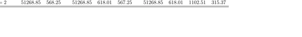
K= 2 51268.85 568.25 51268.85 618.01 567.25 51268.85 618.01 1102.51 315.37
Table 1.5: Estimates of the ICCsand CCCs for PEFR data by number of replicates
[
ICC1 ICC[2 ICC[3 CCC\a CCC\b
K=1 .946 .946 .946 .943 .946
K=2 .957 .957 .948 .945 .948
a
Moment estimator ofCCC without a bias adjustment
b
With adjustment of a bias correction term for estimating (µ1−µ2)2
Table 1.6: Estimates of individual parameters for PEFR data by number of replicates
ˆ
ρ12 ρˆµ12 µˆ1 µˆ2 σˆB21 ˆσ
2
B2 σˆ
2
W1 σˆ
2
W2
K=1 0.94 - 450.35 452.47 - - -
1.4
Discussion
There are several versions of intraclass correlation coefficient discussed in the lit-erature and we summarize these versions in three types for data with only factors of subject and observer. Based on the definition of ICC shown in Section 1.2.1, we compare the expected value of the ICC[ to another popular agreement index CCC under the general model by taking the expectation of the numerator and the denominator of ICC[ for data without and with replications.
We find that the expectation of ICC\1 and ICC\2 depend on the number of repli-cationK, while the expectation ofICC\3 and CCC do not depend on K. In summary, for data without replication (K= 1),E(ICC2) and\ E(ICC3) are essentially the same as\ CCC, while E(ICC1) may be greater or less than\ CCC. For data with replications (K >1), in general, E(ICC\1) and E(ICC\2) are greater than CCC for moderate and large K, and E(ICC\3) =CCC regardless ofK. If data comes from a model where there is subject by observer interaction and the ANOVA model does not include such effect, theICC defined on this model will be biased and will not concur with the CCC defined on a model that accounts for such interaction. Conversely, if the ANOVA model includes all the significant effects the ICC will be the same as the CCC defined on the general model, although in-fluence may be different. In this paper, we only compare the point estimations of ICCs andCCC. Further research is needed to compare the inference of these point estimators to assess the efficiency of estimatingICCsand CCC.
Chapter 2
The random-observers concordance
correlation coefficient
2.1
Introduction
The intraclass correlation coefficient (ICC) and the concordance correlation co-efficient (CCC) are frequently used for assessing agreement between or among observers for data with continuous variables. Usually, theICC and CCC are used for data without and with replications, and they are based on the subject and observer effects only. How-ever, we can not use the methodology if repeated measurements rather than replications are collected. In practice, a true replication, i.e. nothing changed other than the times of the measurements, is often difficult to obtain since it is not easy to maintain the same condition and environment. Oftentimes, repeated measurements rather than replications are taken over time. The time effect should be considered in the measurement in order to account properly different sources of error.
replications, the ICC has been proposed for both random and fixed observers, while the CCC is developed for fixed observer where subjects are treated as random effects. However, there is no CCC for random observers and random time points, while there is a need to develop ICC and CCC type agreement indices with different combinations of random or fixed factors for observers and times.
We investigate CCC agreement index for data with random factors for observers and times since researchers may be interested in assessing many observers who take mea-surements at different time points. For example, when measuring blood pressure, we may want to know whether observers (e.g. nurses) can make reliable measurements at any time, and we are interested in whether these observers can be used interchangeably at any time. Unfortunately, it is difficult or even expensive to use all observers to make measurements at any time. Therefore, observers can be randomly selected from the nurse population to make measurements at randomly selected time points. Since blood pressure fluctuates overtime, their readings should be considered as repeated rather than replicated measurements. Con-sider another example in image study where different observers read the recorded images at different time throughout the day. It is not clear whether the observers can make similar measurements at different times. Thus, there is a need to assess the closeness between mea-surements on the same image by randomly selected observers at randomly selected time. In longitudinal studies, oftentimes different observers are need to take measurements at different follow-up times and we want to make sure these measurements are accurate. Con-sider all observers used in the study as the observer population and time points as the time population and we may consider to establish good agreement between observers from the observer population at different time from the time population.
We propose a new index CCCR for random observers and random time points for
data with repeated measurements. In Section 2.2,CCCRis defined for assessing agreement
in three types. The estimation and statistical inference of CCCR are presented in Section
2.3. In Section 2.4, a simulation study is conducted to evaluate the performance of the CCCRs. The vertebral body data and image data are used to illustrate the proposed
Consider that there are N randomly selected subjects where measurements are taken by J randomly selected observers at K randomly selected time points. For each subject, the random observer and the random time are drawn from observer and time populations, respectively. Let Yijk denote the observed data of subject i measured by
observerjat timek, wherei= 1, ..., N,j= 1, ..., J, andk= 1, ..., K. LetEi(Yijk|j, k) =µjk
and V ari(Yijk|j, k) = σjk2 be the mean and variance of Yijk conditional on subject i by
observer j at time k, where the parameters µjk and σjk2 are random variables because
observers and time are treated as random factors. NotationsEiandV ariare the expectation
and variance respect to subjects forYijk conditional onj andk, respectively.
Vangeneugden et al. (2005) derived severalICC-type agreement indices to assess test-retest, interrater, and absolute reliability coefficients based on linear mixed models. In this section, we proposed random observers and random times forCCC to assess the same three types of agreement, inter-observer, intra-observer and absolute agreement, without assumptions of linear mixed models. The inter-observer agreement is assessing the agree-ment of an observed reading by one rater to an observed reading by a different observer on the same subject at the same time (i.e. Yijk vs Yij′k). The intra-observer agreement
is assessing the agreement of an observed reading on one time to an observed reading on another time by the same observer on the same subject (i.e. Yijk vs Yijk′). The absolute
agreement is assessing the agreement of an observed reading by one observer on one time to an observed reading by a different observer at a different time on the same subject (i.e. Yijk
vsYij′k′). This absolute agreement for data with repeated measurements is similar to total
agreement for data with replicated reading in Barnhart et al. (2005). Both absolute and total agreement contain inter-observer and intra-observer agreement, while absolute agree-ment is for data with repeated measures and total agreeagree-ment is for data with replications. The new indices, CCCR’s, for inter-observer, intra-observer, and absolute agreement are
denoted as CCCinter
R ,CCCRintra, andCCCRabs, respectively, and are described as below.
2.2.1 CCCinter
R for inter-observer agreement
fixed observers as
ρc = 1−
E[(Yi1−Yi2)2]
EI[(Yi1−Yi2)2] ,
whereEIis the conditional expectation given independence ofYi1andYi2. LetYi1k,Yi2k,...,YiJ k
be the measurements made byJ fixed observers where each observer has only one reading for each subject, then Barnhart et al. (2005) extended Lin’s CCC and proposed a total CCC to assess the agreement among multiple observers for data with replications. The total-CCC can be expressed as
ρc(Y) = 1−
PJ−1
j=1
PJ
j′=j+1Ei[(Yijk−Yij′k)2/J(J−1)]
PJ−1
j=1
PJ
j′=j+1EI[(Yijk−Yij′k)2/J(J−1)]
,
where EI is the conditional expectation given independence of Yi1k, Yi2k,..., and YiJ k. By
extending the total-CCC to assess the agreement between random observers at random times for data with repeated measurements, we define the inter-observerCCC for random observer and random time by replacing the summationPJj=1−1PJj′=j+1 with the expectation
Ejj′kfor the new agreement index whereEjj′kis the expectation respect to random observers
j,j′ and random timek. Specifically,
CCCRinter = 1−
Ejj′kEi([Yijk−Yij′k]2|j, j′, k)
Ejj′kEI([Yijk−Yij′k]2|j, j′, k)
, (2.1)
where EI is the conditional expectation given independence of Yijk and Yij′k conditional
on observer and time. With EjkV ari(Yijk|j, k) = Ejkσjk2 = σ2 and V arjkEi(Yijk|j, k) =
V arjkµjk =τ2, we can obtain
Ejj′kEi((Yijk−Yij′k)2|j, j′, k)
= 2σ2+Ejj′k(µjk −µj′k)2−2Ejj′kCovi(Yijk, Yij′k|j, j′, k)
= 2σ2+ 2τ2−2Covjj′k(µjk, µj′k)−(Ejk(µjk)−Ej′k(µj′k))2−2Ejj′kCovi(Yijk, Yij′k|j, j′, k),
and
Ejj′kEI([Yijk−Yij′k]2|j, j′, k) = 2σ2+ 2τ2−2Covjj′k(µjk, µj′k)−(Ejk(µjk)−Ej′k(µj′k))2,
Here we assume that Ejk(µjk) = Ej′k(µj′k), where Ejk(µjk) = EjEk(µjk|j). Then, the
inter-observer agreement for randomCCC can be expressed as
CCCinter
R = 1−
2σ2+ 2τ2−2Covjj′k(µjk, µj′k)−2Ejj′kCovi(Yijk, Yij′k|j, j′, k)
2σ2+ 2τ2−2Cov
jj′k(µjk, µj′k)
= Ejj′kCovi(Yijk, Yij′k|j, j
′, k)
σ2+τ2−Cov
jj′k(µjk, µj′k)
The intra-observerCCC for random observers and random time points is obtained similarly by considering the expected mean square difference for measurements taken on the same subject by the same observer at different time points. We consider two situations for the intra-observer agreement: (1) subjects’ true values do not change over time; (2) subjects’ true values change over time.
If subjects’ true values do not change over time by the same observer with the assumption ofEjk(µjk) =Ejk′(µjk′), the CCCRintra is defined as
CCCintra
R = 1−
Ejkk′Ei([Yijk−Yijk′]2|j, k, k′)
Ejkk′EI([Yijk−Yijk′]2|j, k, k′)
(2.3)
= 1−2σ
2+ 2τ2−2Cov
jkk′(µjk, µjk′)−2Ejkk′Covi(Yijk, Yijk′|j, k, k′)
2σ2+ 2τ2−2Cov
jkk′(µjk, µjk′)
= Ejkk′Covi(Yijk, Yijk′|j, k, k
′)
σ2+τ2−Cov
jkk′(µjk, µjk′)
, (2.4)
whereEI is the conditional expectation given independence ofYijkand Yijk′ conditional on
subject and time.
However, if subjects’ true values change over time, the mean square difference of Yijk−Yijk′ should be replaced by (Yijk−µjk)−(Yijk′ −µjk′) so that the intra-observer
agreement is not affected by the the subjects’ readings taken from time. In this case, the
CCCintra
R can be expressed as
CCCRintra = 1− Ejkk′Ei([(Yijk−µjk)−(Yijk′−µjk′)]
2|j, k, k′)
Ejkk′EI([(Yijk−µjk)−(Yijk′−µjk′)]2|j, k, k′)
(2.5)
= 1−2σ
2−2E
jkk′Covi(Yijk, Yijk′|j, k, k′)
2σ2
= Ejkk′Covi(Yijk, Yijk′|j, k, k
′)
σ2 (2.6)
whereEI is the conditional expectation given independence ofYijkand Yijk′ conditional on
2.2.3 CCCRabs for absolute agreement
The absolute CCC for random observers and random time points is obtained similarly by considering the expected mean square difference for measurements taken on the same subject by different observers at different time points. Here, we also consider two situations for the absolute agreement: (1) subjects’ true values do not change over time; (2) subjects’ true values change over time.
If subjects’ true values do not change over time by different observers with the assumption ofEjk(µjk) =Ej′k′(µj′k′), the CCCRabs is defined as
CCCabs
R = 1−
Ejj′kk′Ei([Yijk−Yij′k′]2|j, j′k, k′)
Ejj′kk′EI([Yijk−Yij′k′]2|j, j′k, k′)
(2.7)
= 1−2σ
2+ 2τ2−2Cov
jj′kk′(µjk, µj′k′)−2Ejj′kk′Covi(Yijk, Yij′k′|j, j′, k, k′)
2σ2+ 2τ2−2Cov
jj′kk′(µjk, µj′k′)
= Ejj′kk′Covi(Yijk, Yij′k′|j, j
′, k, k′)
σ2+τ2−Cov
jj′kk′(µjk, µj′k′)
, (2.8)
where EI is the conditional expectation given independence of Yijk and Yij′k′ conditional
on subject and time.
However, if subjects’ true values may change over time by different observers, the mean square difference of Yijk−Yij′k′ should be replaced by (Yijk−µjk)−(Yij′k′−µj′k′)
so that the absolute agreement is not affected by the the subjects’ readings taken from observers and time. Thus, the CCCabs
R can be expressed as
CCCRabs = 1− Ejj′kk′Ei([(Yijk−µjk)−(Yij′k′ −µj′k′)]
2|j, j′k, k′)
Ejj′kk′EI([(Yijk−µjk)−(Yij′k′ −µj′k′)]2|j, j′k, k′)
(2.9)
= 1−2σ
2−2E
jj′kk′Covi(Yijk, Yij′k′|j, j′, k, k′)
2σ2
= Ejj′kk′Covi(Yijk, Yij′k′|j, j
′, k, k′)
σ2 (2.10)
where EI is the conditional expectation given independence of Yijk and Yij′k′ conditional
To estimate the CCC for random observers and random time points, we used the method of moments approach for each component of CCCR for inter-observer,
intra-observer, and absolute agreement indices. In this section, we present the estimation and inference for CCCinter
R , while CCCRintra and CCCRabs can be done in a similar fashion.
Specifically, the CCCinter
R is estimated by \
CCCinterR =
\
Ejj′kCovi(Yijk, Yij′k|j, j′, k)
ˆ τc2+ ˆσ2
, (2.11)
whereτc2 =τ2−Covjj′k(µjk, µj′k). Note here thatσ2 =EjkV ari(Yijk|j, k) =Ejkσjk2 . Thus,
σjk2 can be estimated by the sample variance conditional on observer j and time k with ˆ
σjk2 =PNi=1(Yijk−Y¯.jk)2/(N−1), and a natural unbiased estimator of σ2 can be estimated
by an average of the sample conditional variance with ˆ
σ2= PJ
j=1 PK
k=1σˆjk2
JK .
The covariance conditional on subject j and time k is Covi(Yijk, Yij′k|j, j′, k), where the
notationCovi is the conditional covariance ofYijk and Yij′k with respect to subjects. Then
Covi(Yijk, Yij′k|j, j′, k) can be estimated by the sample conditional covariance with [
Covi(Yijk, Yij′k|j, j′, k) = N
X
i=1
(Yijk−Y¯.jk)(Yij′k−Y¯.j′k)/(N −1),
and a natural unbiased estimator of the numerator of CCCinter
R can be estimated by an
average of the sample conditional covariance with
\
Ejj′kCovi(Yijk, Yij′k|j, j′, k) = J−1 X
j=1
J
X
j=j′ K
X
k=1
[
Covi(Yijk, Yij′k|j, j′, k)/K
J 2 . Since
Ejj′kEi([ ¯Y.jk−Y¯.j′k]2|j, j′, k)
= Ejj′kV ari([ ¯Y.jk−Y¯.j′k]|j, j′, k) +Ejj′k(µjk−µj′k)2
= 1
NEjj′k(σ 2
jk+σ2j′k−2Covi(Yijk, Yij′k|j, j′k)) +Ejj′k(µjk−µj′k)2
= 2
N(σ 2−E
jj′kCovi(Yijk, Yij′k|j, j′k)) + 2τ2−2Covjj′k(µjk, µj′k)
= 2
N(σ 2−E
with the assumption of Ejk(µjk) = Ej′k(µj′k), then the expression of τc2 form the above
equation can be written as τc2= 1
2Ejj′kEi([ ¯Y.jk−Y¯.j′k]
2|j, j′k)− 1
N[σ 2−E
jj′kCovi(Yijk, Yij′k|j, j′k)].
Thus, a natural unbiased estimator of τc2 can be estimated by plugging in the estimates of ˆ
σ2 and Ejj\′kCovi(Yijk, Yij′k|j, j′, k) as
ˆ τc2=
PJ−1
j=1
PJ j=j′
PK
k=1( ¯Y.jk−Y¯.j′k)2
2K J2 −
1 N[bσ
2−E\
jj′kCovi(Yijk, Yij′k|j, j′, k)].
In order to deal with the inference ofCCCRand easily construct confidence
inter-vals for inter-observer, intra-observer, and absolute agreement, we consider the bootstrap method for the three agreement indices. Efron and Tibshirani (1993) described several different approaches of confidence intervals based on the use of bootstrap method without asymptotically normality assumptions or other complex properties for the point estima-tor. The percentile method and bootstrap-t method are useful for constructing such con-fidence intervals. Some complex methods are based on the percentile version which may improve the coverage probability, such as bias-corrected and accelerated method (BCα)
and approximate bootstrap conf idencemethod (ABC). However, in our simulation stud-ies, we found that the percentile method,BCα method, andABC method did not perform
well. Below we describe the bootstrap-tmethod for constructing a 95% bootstrap confidence interval. We make a minor modification for the bootstrap-tmethod since this method pre-sented in Efron’s book is usually suitable only for some simple statistics, such as the sample mean and sample median. We present the modified bootstrap-tmethod for the confidence interval of CCCinter
R because of its better performance in our simulation studies; the same
method for constructing the confidence interval can be used for CCCRintra and CCCRabs, respectively.
Let (k1b, k2b, ..., kKb), (j1b, j2b, ..., jJ b), and (i1b, i2b, ..., iN b) be the bth bootstrap
sample drawn with replacement from indices of times (1, ..., K), observers (1, ..., J), and subjects (1, ..., N), respectively. The B independent bootstrap data sets can be obtained by {Yiibjjbkkb, i = 1, ..., N;j = 1, ..., J;k = 1, ..., K}, where b = 1, ..., B. The CCCRinter for each bootstrap sample is estimated by
\
CCCinterR (b) = Ejj\′kCovi(Yiibjjbkkb, Yiibj′j′bkkb|j, j
′, k)
ˆ τ2
cb+ ˆσ2b
strap sample. The 100(1-2α)% bootstrap-tconfidence interval of CCCR is defined as
(\CCCinterR −ˆt(1−α)·se,ˆ \CCCinterR −tˆ(α)·se),ˆ (2.13)
where ˆt(α) refers to the αth percentile of (\CCCinter
R (b) −\CCC
inter
R )/se(b), where ˆˆ se is
the estimated standard error of \CCCinterR , and ˆse(b) is the estimated standard error of
\
CCCinterR (b) for the bootstrap sample Yiibjjbkkb. However, unlike the examples in Efron’s
book, we do not find a formula for the estimated standard error of CCC\interR . Thus, we approximate ˆseby ˆse(b) to obtain the the 100(1-2α)% confidence interval ofCCCinter
R as
(\CCCinterR −tˆ(1−α)·se(b),ˆ \CCCinterR −tˆ(α)·se(b)).ˆ (2.14)
2.4
Simulations
To evaluate the performance of CCCRabs, CCCRinter, and CCCRintra for random observers and random time, we carried out simulations based on 1000 Monte Carlo data sets. We consider that the number of observers drawn form the observer population is 2, 4, 6, respectively (J = 2,4,6), and three time points (K = 3) for each observer are randomly drawn from the time population. The sample size of subjects for each combination of the number of observers and time points is 20, 50, 100, 150, 200, 250, 300, and 500, respectively. To illustrate the process of generating the data set, consider the situation with two random observers (J = 2) and three random time points (K = 3). Assume that the observer population has normal distribution with meanµand variance σ2
µ. Two observers’
overall mean parameters µ1 and µ2 were randomly selected from the observer population N(µ, σ2µ). For a given observer j, we generated µjk at random time k withEk(µjk|j) =µj
and V ark(µjk|j) = σ2µj, where σ 2
µj was generated from a gamma distribution with σ 2
µj ∼
Gamma(σ20,1),j= 1,2. We will use the following assumptions for the correlations ofµjk’s
(1) Corr(µjk, µjk′) =ρ1, (2) Corr(µjk, µj′k) =ρ2, and (3) Corr(µjk, µj′k′) =ρ1ρ2, where
with mean (µ1, µ1, µ1, µ2, µ2, µ2)T and variance-covariance matrix
Σ6µ×6=
σ2
µ1 ρ1σ
2
µ1 ρ1σ
2
µ1 ρ2σµ1σµ2 ρ1ρ2σµ1σµ2 ρ1ρ2σµ1σµ2
ρ1σµ21 σ 2
µ1 ρ1σ
2
µ1 ρ1ρ2σµ1σµ2 ρ2σµ1σµ2 ρ1ρ2σµ1σµ2
ρ1σµ21 ρ1σ 2
µ1 σ
2
µ1 ρ1ρ2σµ1σµ2 ρ1ρ2σµ1σµ2 ρ2σµ1σµ2
ρ2σµ1σµ2 ρ1ρ2σµ1σµ2 ρ1ρ2σµ1σµ2 σ 2
µ2 ρ1σ
2
µ2 ρ1σ
2
µ2
ρ1ρ2σµ1σµ2 ρ2σµ1σµ2 ρ1ρ2σµ1σµ2 ρ1σ 2
µ2 σ
2
µ2 ρ1σ
2
µ2
ρ1ρ2σµ1σµ2 ρ1ρ2σµ1σµ2 ρ2σµ1σµ2 ρσ 2
µ2 ρ1σ
2
µ2 σ
2 µ2 .
Finally, the observed data (Yi11, Yi12, Yi13, Yi21, Yi22, Yi23)T for each subject i was generated from a multivariate normal distribution with mean (µ11, µ12, µ13, µ21, µ22, µ23)T and variance covariance matrix
Σ6×6
=
σ211 ρ1σ11σ12 ρ1σ11σ13 ρ2σ11σ21 ρ1ρ2σ11σ22 ρ1ρ2σ11σ23 ρ1σ12σ11 σ122 ρ1σ122 σ13 ρ1ρ2σ12σ21 ρ2σ12σ22 ρ1ρ2σ12σ23 ρ1σ13σ11 ρ1σ13σ12 σ213 ρ1ρ2σ13σ21 ρ1ρ2σ13σ22 ρ2σ13σ23 ρ2σ11σ21 ρ1ρ2σ11σ22 ρ1ρ2σ11σ23 σ212 ρ1σ21σ22 ρ1σ21σ23 ρ1ρ2σ12σ21 ρ2σ12σ22 ρ1ρ2σ12σ23 ρ1σ22σ21 σ222 ρ1σ22σ23 ρ1ρ2σ13σ21 ρ1ρ2σ13σ22 ρ2σ13σ23 ρσ23σ21 ρ1σ23σ22 σ223
,
whereσ2
jkwas generated from a gamma distribution withσjk2 ∼Gamma(σT2,1),j = 1,2, k=
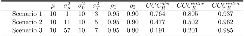
1,2,3. With these assumptions, we have σ2 =σ2T and τc2 = σ2µ+σ02. Table 2.1 shows the true values ofµ,σµ2,σ02,σT2,ρ1, andρ2used for data generation as well as the corresponding true values of CCCR. The true values of CCCRabs and CCCRinter provide situations with
strong, moderate, and mild agreement between observers, and the true values ofCCCintra R
represents strong agreement within observers.
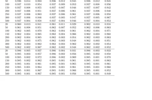
We evaluate the performance ofCCCRfor inter-observer, intra-observer, and
abso-lute agreement based on 1000 Monte Carlo data sets by calculating (1) the average estimates ofCCCR, (2) the standard deviation of the estimates ofCCCR, and (3) the coverage
prob-ability for a modified 95% bootstrap-t confidence interval. The results are shown in Table 2.3-2.4 for J = 2,4,6, respectively, which indicate that the bias of the point estimate of CCCR decreases as the sample size and the number of observers increase. The estimate is
µ σµ σ0 σT ρ1 ρ2 CCCR CCCR CCCR
Scenario 1 10 1 10 3 0.95 0.90 0.764 0.805 0.937 Scenario 2 10 11 10 5 0.95 0.90 0.477 0.502 0.962 Scenario 3 10 57 10 7 0.95 0.90 0.191 0.201 0.985
Table 2.2: Results ofCCCRabs based on 1000 Monte Carlo data sets
CCCabs
R J=2 J=4 J=6
N Mean SD Coverage Mean SD Coverage Mean SD Coverage
0.764 20 0.773 0.098 0.851 0.778 0.075 0.837 0.778 0.075 0.835
50 0.770 0.055 0.894 0.770 0.044 0.894 0.773 0.039 0.892
100 0.769 0.038 0.936 0.767 0.030 0.925 0.768 0.028 0.938
150 0.768 0.030 0.945 0.767 0.024 0.933 0.767 0.024 0.952
200 0.766 0.025 0.959 0.766 0.021 0.936 0.766 0.020 0.951
250 0.765 0.022 0.967 0.766 0.019 0.942 0.765 0.017 0.948
300 0.765 0.021 0.976 0.765 0.017 0.937 0.765 0.016 0.954
500 0.765 0.016 0.973 0.765 0.013 0.955 0.764 0.012 0.946
0.477 20 0.463 0.174 0.854 0.469 0.132 0.869 0.471 0.106 0.881
50 0.475 0.108 0.893 0.479 0.072 0.916 0.475 0.065 0.925
100 0.476 0.074 0.916 0.478 0.052 0.935 0.479 0.045 0.942
150 0.476 0.061 0.932 0.478 0.042 0.939 0.478 0.036 0.931
200 0.476 0.054 0.951 0.478 0.037 0.955 0.478 0.032 0.950
250 0.476 0.046 0.944 0.477 0.032 0.947 0.478 0.029 0.941
300 0.476 0.042 0.948 0.477 0.029 0.952 0.478 0.025 0.945
500 0.476 0.034 0.960 0.477 0.023 0.947 0.477 0.020 0.948
0.191 20 0.183 0.220 0.861 0.187 0.115 0.863 0.188 0.094 0.850
50 0.186 0.137 0.909 0.187 0.072 0.914 0.188 0.057 0.914
100 0.188 0.095 0.926 0.192 0.053 0.926 0.193 0.041 0.928
150 0.188 0.078 0.927 0.192 0.042 0.948 0.189 0.032 0.950
200 0.190 0.068 0.938 0.192 0.038 0.945 0.190 0.029 0.942
250 0.190 0.062 0.944 0.189 0.034 0.946 0.190 0.027 0.931
300 0.192 0.054 0.939 0.191 0.030 0.942 0.191 0.025 0.948
Table 2.3: Results ofCCCRinter based on 1000 Monte Carlo data sets
CCCinter
R J=2 J=4 J=6
N Mean SD Coverage Mean SD Coverage Mean SD Coverage
0.805 20 0.824 0.089 0.827 0.820 0.068 0.845 0.824 0.061 0.826
50 0.812 0.050 0.896 0.814 0.037 0.898 0.812 0.035 0.891
100 0.809 0.033 0.916 0.809 0.024 0.925 0.809 0.024 0.918
150 0.809 0.027 0.925 0.807 0.021 0.943 0.807 0.019 0.932
200 0.808 0.024 0.930 0.807 0.018 0.937 0.807 0.016 0.942
250 0.807 0.020 0.937 0.806 0.016 0.948 0.805 0.015 0.947
300 0.806 0.019 0.947 0.805 0.015 0.943 0.805 0.013 0.938
500 0.806 0.014 0.951 0.805 0.011 0.961 0.805 0.010 0.949
0.502 20 0.498 0.174 0.858 0.502 0.119 0.869 0.503 0.106 0.873
50 0.499 0.110 0.889 0.500 0.070 0.921 0.500 0.063 0.909
100 0.499 0.074 0.937 0.502 0.050 0.945 0.503 0.042 0.940
150 0.500 0.059 0.932 0.504 0.041 0.940 0.501 0.034 0.942
200 0.501 0.052 0.938 0.504 0.036 0.953 0.502 0.032 0.951
250 0.501 0.045 0.942 0.500 0.031 0.951 0.503 0.028 0.958
300 0.503 0.043 0.953 0.500 0.031 0.958 0.503 0.025 0.951
500 0.503 0.033 0.955 0.503 0.022 0.955 0.502 0.020 0.949
0.201 20 0.199 0.218 0.862 0.199 0.120 0.862 0.202 0.094 0.865
50 0.197 0.135 0.918 0.198 0.072 0.911 0.199 0.057 0.922
100 0.199 0.095 0.937 0.200 0.054 0.945 0.199 0.041 0.927
150 0.199 0.079 0.936 0.201 0.042 0.942 0.199 0.032 0.943
200 0.199 0.068 0.955 0.201 0.037 0.953 0.200 0.029 0.935
250 0.200 0.060 0.948 0.201 0.032 0.941 0.202 0.025 0.950
300 0.199 0.055 0.943 0.201 0.030 0.948 0.201 0.023 0.948
Table 2.4: Results of CCCRintra based on 1000 Monte Carlo data sets
CCCintra
R J=2 J=4 J=6
N Mean SD Coverage Mean SD Coverage Mean SD Coverage
0.937 20 0.933 0.026 0.925 0.933 0.022 0.917 0.935 0.020 0.918
50 0.936 0.014 0.933 0.936 0.012 0.945 0.936 0.012 0.945
100 0.937 0.010 0.954 0.937 0.009 0.953 0.937 0.008 0.956
150 0.937 0.008 0.955 0.937 0.007 0.946 0.937 0.007 0.942
200 0.937 0.006 0.951 0.937 0.006 0.961 0.937 0.006 0.940
250 0.937 0.006 0.963 0.937 0.006 0.961 0.937 0.006 0.958
300 0.937 0.006 0.946 0.937 0.005 0.947 0.937 0.005 0.967
500 0.937 0.004 0.958 0.937 0.004 0.946 0.937 0.004 0.953
0.962 20 0.960 0.013 0.941 0.961 0.011 0.929 0.962 0.010 0.916
50 0.961 0.008 0.951 0.962 0.007 0.952 0.962 0.006 0.963
100 0.962 0.005 0.970 0.962 0.004 0.961 0.962 0.004 0.971
150 0.962 0.004 0.965 0.962 0.004 0.966 0.962 0.003 0.968
200 0.962 0.004 0.965 0.962 0.003 0.954 0.962 0.003 0.963
250 0.962 0.003 0.975 0.962 0.003 0.948 0.962 0.003 0.951
300 0.962 0.003 0.962 0.962 0.003 0.962 0.962 0.002 0.954
500 0.962 0.002 0.967 0.962 0.002 0.948 0.962 0.002 0.952
0.985 20 0.986 0.005 0.937 0.986 0.004 0.931 0.986 0.003 0.933
50 0.985 0.003 0.957 0.986 0.002 0.956 0.985 0.002 0.958
100 0.985 0.002 0.972 0.986 0.002 0.969 0.985 0.001 0.970
150 0.985 0.002 0.962 0.985 0.001 0.961 0.985 0.001 0.963
200 0.985 0.001 0.961 0.985 0.001 0.965 0.985 0.001 0.961
250 0.985 0.001 0.964 0.985 0.001 0.961 0.985 0.001 0.960
300 0.985 0.001 0.967 0.985 0.001 0.966 0.985 0.001 0.952
2.5.1 Vertebral Body Data
We first use data from a vertebral body wedging study of pediatric patients. The data was measured in thoracic and lumbar area of vertebral body at the thoracolumbar junction for patients with ages between 0 and 17 years. Anterior and posterior vertebral body heights were measure by two experienced pediatric radiologists on six locations (T10, T11, T12, L1, L2, L3) of the vertebral body, providing a combination of the 12 locations measured for each patient. In all 100 patients measured by two radiologists, 20 patients were measured twice by the same radiologists and the remaining 80 patients were measured only once by each of the two radiologists. For illustration of the proposed methodology, we use this data set to determine the degree of the inter-observer, intra-observer, and absolute agreement between two radiologists in two situations below. In both situations, we assumed that two radiologists (J = 2) were randomly selected from the pediatric radiologists pop-ulation. However, in the first situation, the time points are the two times when the same radiologists make measurements for the 20 patients. In the second situation, we consider the 12 locations as the ”time points” where each of the two radiologists make measurements for all 100 patients. Because the radiologists made measurements twice in the first 20 patients, only the first measurement is used in this situation.
Situation 1: Two random time points
95% bootstrap-tconfidence intervals for inter-rater, intra-rater, and absolute agreement at each location. The results indicate similar agreement between two radiologists across 12 locations. In order to construct the common estimates of CCCR across locations in this
situation, we take the average of the 12 estimates of CCCR as
¯
\
CCCR to be the estimate
for the common estimate of CCCR. We use the modified bootstrap-t method to
estab-lish the 95% confidence interval for the common estimates of inter-observer, intra-observer and absolute agreement, respectively. Specifically, for assessing the inter-observer agree-ment, a total 200 independent bootstrap samples (B = 200) were drawn with replacement from indices of two time points, two radiologists, and 17 subjects, respectively. For each bootstrap samples,\CCCinterR1 (b), \CCCinterR2 (b), ..., \CCCinterR12 (b) are the 12 estimates for the inter-observer agreement for each bootstrap b, b = 1, ...,200. We then take the average of the 12 estimates as \CCC¯ interR (b) to obtain the estimate for the common estimate for each bootstrap b. Then, the final 95% confidence interval is obtained by
(\CCC¯ interR −t¯ˆ(1−α)·se(b),ˆ¯ \CCC¯ interR −t¯ˆ(α)·se(b)),¯ˆ (2.15)
where ¯ˆt(α) is the αth percentile of (\CCC¯ interR (b)−
¯
\
CCCinterR )/se(b), and ¯ˆ¯ˆ se(b) is the
esti-mated standard error of\CCC¯ interR (b); the confidence intervals for the common estimates of
\
CCCintraR and \CCCabsR can be obtained similarly and the results are shown in Table 2.8.
Situation 2: Random time points as random locations
In the second situation, We considered all 100 patients measured by two radiologists (J = 2) on the 12 locations (K = 12), where the locations are treated as repeated measurements randomly selected from the location population. For illustration, the data was restricted to the 90 subjects (N = 90) without missing data by two radiologists at 12 locations. Fig-ures 2.5-2.6 showed the scatter plots for the comparisons between two radiologists for the measurements at the 12 locations. The scatter plots showed that overall measurements of two radiologists scattered more closely to the 45◦ line on all levels, respectively. Table 2.8 showed the point estimates of CCCRs with the corresponding modified 95% bootstrap-t
confidence interval for inter-rater, intra-rater, and absolute agreement. The results indi-cate similar agreement between two radiologists. Here, since the subjects’ true values may change over ”time”, for calculating the estimates ofCCCabs
and (Yijk−µjk) −(Yijk′ −µjk′), respectively in order to exclude the situation that the
agreement may affect by the subjects’ readings from time.
Note that the common CCCR in Situation 1 assesses agreement between
radi-ologists aggregated over the locations where the locations are treated as fixed, while the CCCR in Situation 2 assesses the agreement between radiologists over all possible locations
where locations are treated as random. Thus, the estimates of CCCR in Situation 2 are
lower than that of the common CCCR in Situation 1 because random locations can cause
lower agreement between radiologists. In both situations for the study of the vertebral body data, the estimates of CCCinter
R in Table 2.8 are almost the same as the estimates ofρc,rm
Table 2.5: Description statistics for readings between times by readers and locations in Situation 1 for vertebral body data
Location Reader 1 Reader 2
Anterior(A)/Posterior(P) 1st Read 2nd Read Diff 1st Read 2nd Read Diff
T10 A mean(sd) 17.971(5.212) 18.518(4.866) -0.547(1.546) 18.765(5.640) 18.000(4.988) 0.765(1.322)
min(max) 8.4(28.4) 9.0(25.0) -2.6(3.4) 8.7(27.0) 9.3(25.0) -1.4(2.9)
T10 P mean(sd) 18.276(5.210) 18.553(4.516) -0.276(1.602) 19.559(5.898) 18.388(4.674) 1.171(1.987)
min(max) 9.0(28.6) 9.0(24.6) -2.2(4.8) 9.3(27.0) 9.4(24.3) -1.9(6.4)
T11 A mean(sd) 18.800(5.492) 19.129(5.367) -0.329(1.750) 19.459(6.189) 18.959(5.465) 0.500(1.470)
min(max) 8.1(27.6) 8.7(27.3) -2.5(5.0) 8.7(28.2) 8.8(27.1) -2.6(3.4)
T11 P mean(sd) 19.324(5.669) 19.647(5.398) -0.324(1.649) 20.400(6.055) 19.441(5.614) 0.959(2.038)
min(max) 8.4(28.3) 9.0(27.3) -2.9(4.1) 9.3(28.6) 9.1(28.6) -2.0(7.5)
T12 A mean(sd) 20.394(5.780) 20.012(5.691) 0.382(1.364) 20.276(5.859) 19.759(5.386) 0.518(1.204)
min(max) 9.8(28.5) 10.5(29.7) -1.6(3.3) 10.2(28.1) 10.6(27.6) -0.7(3.7)
T12 P mean(sd) 20.712(5.752) 20.694(5.637) 0.018(1.160) 20.976(6.182) 20.418(5.748) 0.559(1.971)
min(max) 10.4(29.0) 11.1(30.8) -2.1(2.0) 10.1(28.9) 10.8(29.9) -3.2(5.3)
L1 A mean(sd) 21.400(6.284) 21.124(5.720) 0.276(1.186) 21.424(6.322) 20.888(5.431) 0.535(1.556)
min(max) 9.9(31.8) 10.5(28.3) -1.6(3.5) 10.2(31.0) 10.8(29.4) -1.5(4.5)
L1 P mean(sd) 21.988(6.683) 21.600(5.698) 0.388(1.488) 22.088(6.562) 21.800(5.801) 0.288(1.661)
min(max) 10.1(32.2) 11.0(29.6) -2.8(2.6) 10.1(31.9) 11.1(31.0) -2.1(4.1)
L2 A mean(sd) 22.694(6.569) 21.971(6.224) 0.724(2.063) 22.041(6.205) 21.924(6.071) 0.118(0.926)
min(max) 10.1(33.1) 11.0(30.7) -2.2(4.7) 10.7(30.5) 10.7(29.8) -1.3(2.1)
L2 P mean(sd) 23.224(6.717) 22.147(6.010) 1.076(2.238) 22.471(6.588) 22.471(6.323) 0.000(1.280)
min(max) 9.6(33.1) 11.3(30.5) -1.9(5.2) 10.1(32.2) 11.1(31.5) -1.9(2.9)
L3 A mean(sd) 22.759(6.866) 22.518(6.561) 0.241(1.738) 22.082(6.676) 21.988(6.382) 0.094(1.163)
min(max) 9.6(32.7) 10.4(31.7) -2.4(4.7) 10.1(32.0) 9.6(31.3) -1.3(3.4)
L3 P mean(sd) 22.988(6.924) 22.371(6.418) 0.617(1.414) 22.329(6.805) 22.041(6.176) 0.288(1.907)
Table 2.6: Description statistics for readings between readers by times and locations in Situation 1 for vertebral body data
Location 1st Read 2nd Read
Anterior(A)/Posterior(P) Reader 1 Reader 2 Diff Reader 1 Reader 2 Diff
T10 A mean(sd) 17.971(5.212) 18.765(5.640) -0.794(1.682) 18.518(4.866) 18.000(4.988) 0.518(0.993)
min(max) 8.4(28.4) 8.7(27.0) -3.2(1.5) 9.0(25.0) 9.3(25.0) -1.5(2.2)
T10 P mean(sd) 18.276(5.210) 19.559(5.898) -1.282(1.878) 18.553(4.516) 18.388(4.674) 0.165(1.013)
min(max) 9.0(28.6) 9.3(27.0) -5.4(1.6) 9.0(24.6) 9.4(24.3) -1.6(1.9)
T11 A mean(sd) 18.800(5.492) 19.459(6.189) -0.658(1.678) 19.129(5.367) 18.959(5.465) 0.171(1.484)
min(max) 8.1(27.6) 8.7(28.2) -3.8(2.0) 8.7(27.3) 8.8(27.1) -2.6(2.9)
T11 P mean(sd) 19.324(5.669) 20.400(6.055) -1.076(1.720) 19.647(5.398) 19.441(5.614) 0.206(1.614)
min(max) 8.4(28.3) 9.3(28.6) -4.4(2.4) 9.0(27.3) 9.1(28.6) -4.2(3.4)
T12 A mean(sd) 20.394(5.780) 20.276(5.859) 0.117(1.097) 20.012(5.691) 19.759(5.386) 0.253(1.219)
min(max) 9.8(28.5) 10.2(28.1) -2.9(1.8) 10.5(29.7) 10.6(27.6) -2.2(2.3)
T12 P mean(sd) 20.712(5.752) 20.976(6.182) -0.265(1.412) 20.694(5.637) 20.418(5.748) 0.276(1.468)
min(max) 10.4(29.0) 10.1(28.9) -3.8(1.8) 11.1(30.8) 10.8(29.9) -3.4(2.9)
L1 A mean(sd) 21.400(6.284) 21.424(6.322) -0.023(1.264) 21.124(5.720) 20.888(5.431) 0.235(1.340)
min(max) 9.9(31.8) 10.2(31.0) -2.7(1.7) 10.5(28.3) 10.8(29.4) -1.2(4.7)
L1 P mean(sd) 21.988(6.683) 22.088(6.562) -0.100(1.352) 21.600(5.698) 21.800(5.801) -0.200(1.337)
min(max) 10.1(32.2) 10.1(31.9) -2.6(2.2) 11.0(29.6) 11.1(31.0) -2.1(3.7)
L2 A mean(sd) 22.694(6.569) 22.041(6.205) 0.653(2.089) 21.971(6.224) 21.924(6.071) 0.047(1.693)
min(max) 10.1(33.1) 10.7(30.5) -3.9(3.3) 11.0(30.7) 10.7(29.8 ) -3.1(2.5)
L2 P mean(sd) 23.224(6.717) 22.471(6.588) 0.753(1.692) 22.147(6.010) 22.471(6.323) -0.324(1.538)
min(max) 9.6(33.1) 10.1(32.2) -2.5(3.4) 11.3(30.5) 11.1(31.5) -2.8(2.3)
L3 A mean(sd) 22.759(6.866) 22.082(6.676) 0.676(1.541) 22.518(6.561) 21.988(6.382) 0.529(1.244)
min(max) 9.6(32.7) 10.1(32.0) -2.4(3.2) 10.4(31.7) 9.6(31.3) -2.3(3.1)
L3 P mean(sd) 22.988(6.924) 22.329(6.805) 0.659(1.457) 22.371(6.418) 22.041(6.176) 0.329(1.529)
Table 2.7: Description statistics for readings between readers and times by locations in Situation 1 for ve