ABSTRACT
THORSEN, WAVERLY ANNE. Bioavailability of Particulate-Sorbed Polycyclic Aromatic
Hydrocarbons. (Under the direction of Drs. Damian Shea and W. Gregory Cope).
Understanding the behavior of contaminants in the environment is essential for an
adequate assessment of a chemicals’ fate, subsequent exposure to organisms, and potential
for toxic effects. However, contaminant behavior can be complex, involving multiple
interactions such as sorption to, and desorption from, particles present in the water column
and sediment phase, competition for binding sites, and sequestration deep within particle
pores, altering the chemical and biological availability of the contaminants. Therefore, one
way to understand a contaminants’ behavior in the environment is to assess its
bioavailability, or fraction of contaminant available for uptake by organisms. This is
generally accomplished by measuring the concentration of a contaminant present in
organism tissue, and comparing it to concentrations in different environmental
compartments (water, sediment).
In this study, numerous toxicokinetic parameters, bioconcentration factors
and biota-sediment accumulation factors for 46 polycyclic aromatic hydrocarbons in
freshwater mussels were measured. Elimination rates ranged from 0.04 (perylene) to
0.26/day (2,6-dimethylnapthalene), half-lives ranged from 2.6 to 16.5 days, and times to
reach 95% of steady-state ranged from 11.3 to 71.3 days. The ranges and individual values
compare well to available published literature values.
Bioconcentration factors ranged from 1.54 (naphthalene) to 5.20 (coronene),
depending on individual analyte and study conditions, but generally increased with
concentrations of dissolved and particulate organic carbon present in the water column, and
to partition coefficients used to account for these parameters. Additionally, biota-sediment
accumulation factors demonstrated that pyrogenic PAH (associated with
incomplete-combustion) have much lower bioavailability than petrogenic PAH (associated with
petroleum), with average values ranging from 0.55 +/-0.049 to 2.44 +/- 1.15, respectively.
Moreover, PAH bioavailability was dependent on concentrations of soot carbon in the
environment as well as the specific source of the PAH (petrogenic vs pyrogenic). This is the
BIOAVAILABILITY OF PARTICULATE-SORBED POLYCYCLIC AROMATIC HYDROCARBONS
By
WAVERLY ANNE THORSEN
A dissertation submitted to the Graduate Faculty of North Carolina State University
in partial fulfillment of the requirements for the Degree of
Doctor of Philosophy
DEPARTMENT OF ENVIRONMENTAL AND MOLECULAR TOXICOLOGY
Raleigh
2003
APPROVED BY:
Dr. Ross B. Leidy Dr. Michael Stoskopf
Dr. W. Gregory Cope Dr. Damian Shea
BIOGRAPHY
Waverly Anne Thorsen was born Waverly Anne Watson and raised in Hanover, New
Hampshire. Her interest in science began in high school and continued at Bowdoin College
in Brunswick, ME, where she majored in chemistry. Throughout college she pursued her love
of science and the outdoors, both in the classroom and through summer jobs. This included
time as a hiking guide on the Appalachian Trail (for the Appalachian Mountain Club), as
well as work as a summer student/laboratory technician at Los Alamos National Laboratory
in New Mexico. Waverly’s senior thesis at Bowdoin involved work with marine mussels as
indicator organisms for measurement of hydrocarbon residues at the site of an oil spill off the
coast of Maine. This work led directly to her enrollment at North Carolina State University in
the Department of Environmental and Molecular Toxicology. At NCSU, Waverly focused on
studying the bioavailability of certain classes of environmental organic contaminants to
aquatic organisms, such as freshwater mussels. She was particularly interested in
understanding interactions between organic contaminants and various sediment components
such as organic carbon and soot carbon, and the ultimate effects they have on contaminant
bioavailability. Apart from her academic goals, Waverly enjoys multiple outdoor pursuits
ACKNOWLEDGEMENTS
I would like to thank the many people that aided me in completing this dissertation: to my
fellow Chemical Exposure Assessment laboratory members for their support, encouragement
and advice, particularly Peter R. Lazaro; to the administrative staff who helped with the
numerous purchase orders, curriculum requirements, exam scheduling, and always offered
friendly concern and care; and to my advisors, committee members and professors for their
TABLE OF CONTENTS
Page
List of Tables………..xi
List of Figures………...xiii
List of Abbreviations/Symbols……….xiv
Chapter 1: Toxicokinetics of Environmental Contaminants in Freshwater Mussels..1
Introduction………..2
Uptake and Elimination………...4
Bioconcentration………..6
Bioaccumulation-BAF and BSAF………...8
Metabolism and Biotransformation………...10
Bioavailability and Biotic-Ligand Model………..10
Chemical Classes………...12
I. Hydrophobic Organic Contaminants………..12
Uptake………12
Bioconcentration………18
Elimination……….23
Attainment of Steady-state……….26
Bioaccumulation and Bioavailability……….27
Implications and Potential for HOC Toxicity to Freshwater Mussels………..30
II. Metals………31
Uptake (Overview)……….31
Cadmium………33
Uptake and Accumulation………..33
Steady-state and Bioconcentration……….35
Elimination……….37
Mercury………..37
Uptake and Accumulation………..37
Elimination……….39
Lead………39
Uptake and Accumulation………..39
Elimination……….40
Silver………..41
Uptake and Accumulation………..41
Elimination……….42
Nickel……….42
Tin………..43
Uptake and Accumulation………..43
Elimination……….44
Metal Mixtures and Effects on Toxicokinetics………..45
Platinum Group Metals………..46
Essential Elements……….47
Zinc, Calcium, Copper………...47
Metal Detoxification Mechanisms……….50
Implications and Potential for Metal Toxicity………...51
References………..52
Tables……….64
Figure Legends………...73
Figures………74
Chapter 2: Elimination Rate Constants for 46 PAHs in Elliptio complanata………78
Abstract………..79
Introduction………79
Methods………..82
Field Collection and Experimental Design………82
Monitoring of Water Quality Parameters………..84
Tissue PAH Extraction and Analysis………85
Quality Control and Quality Assurance Protocol………..86
Results………86
Discussion………..88
Comparison of K2 and other kinetic parameters to literature values…….88
First-order vs Second-order Elimination Kinetics……….89
Relationship Between K2 and log Kow………...90
Reasoning Behind apparent Plateau in K2 values at log Kow>6………….91
Effect of Stress on Kinetics………92
Tables……….95
Figure Legends………...98
Figures………99
Chapter 3: Effects of DOC and POC on PAH Bioavailability: Sensitivity of BCFs to Exposure Environment………..102
Abstract………103
Introduction………..104
Methods………107
Study Designs………..107
Study A………108
Study B………108
Study C………109
Extraction Procedures and Instrumentation……….110
Water Samples……….110
Mussel Samples………...110
Sample Quantification……….112
Quality Control and Quality Assurance Protocol………112
Results………..113
Calculation and Comparison of BCF values………113
Calculation of Steady-State Bioconcentration Regression Equations….113 Discussion………115
Comparison of Regression Equations Calculated with Different KDOC, KPOC
Values……….117
Effect of Different KDOC, KPOC on Predicted Water Concentrations…...121
Effect of Different DOC, POC Concentrations on Predicted Water Concentrations……….124
Conclusions………..126
References………126
Tables………...130
Chapter 4: Bioavailability of PAHs: Effects of Soot Carbon and PAH Source…...138
Abstract………139
Introduction………..140
Methods………144
Sample Collection-Freshwater Sites………144
Sample Collection-Marine Sites………..144
Sample Extraction………145
Sample Analytical PAH Analysis………145
Results and Discussion………146
Calculation of BSAF Values and Assessment of Bioavailability………146
Consideration of PAH Hydrophobicity………...149
Other Considerations of Decreased BSAF Values………..150
Consideration of Soot Carbon (SC) as an Additional Sediment Sorptive Phase………152
Variation of PAH Source and Subsequent Effect on Bioavailability…..155
Acknowledgements………..158
References………158
Tables………...161
Figure Legends……….164
LIST OF TABLES
Page
Chapter 1.Toxicokinetics of Environmental Contaminants in Freshwater Mussels
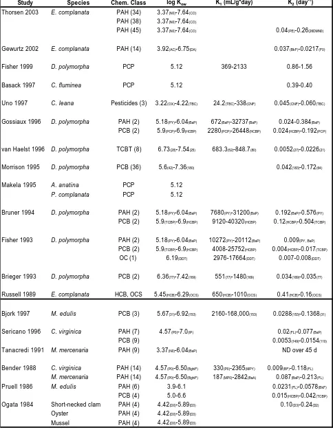
Table 1(a). Comparison of hydrophobic organic contaminant uptake rates and elimination rates for freshwater and marine mussel species across various studies ………64
Table 1(b). Comparison of hydrophobic organic contaminant BCF and half-life values for freshwater and marine mussel species across various studies………...65
Table 2 (a). Literature list of toxicokinetic studies of hydrophobic organic contaminants on mussels: exposure, chemical class, study duration………...66
Table 2 (b). Literature list of toxicokinetic studies or hydrophobic organic contaminants on mussels: miscellaneous information and parameters measured……...67
Table 3. List of numerous individual hydrophobic organic contaminants across studies for direct comparison of toxicokinetic parameters………..68
Table 4. Comparison of steady-state bioconcentration regression equations for organic contaminants in mussels………69
Table 5. List of complex interactions between mussel, water and sediment that influence speciation, behavior and accumulation of metals………..70
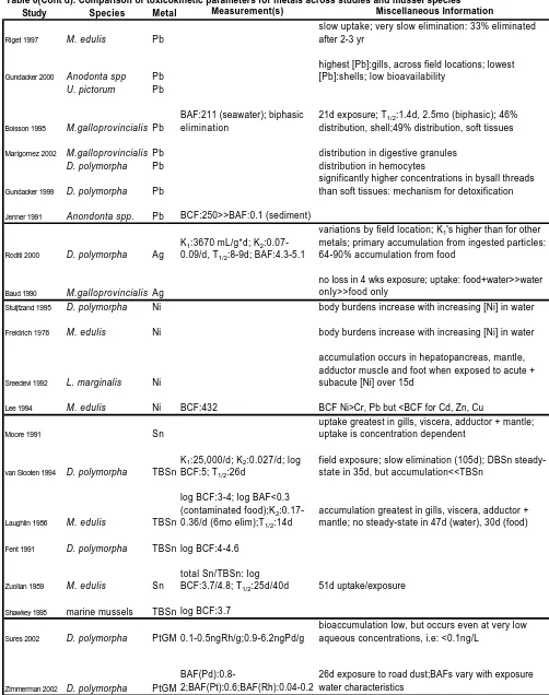
Table 6. Comparison of metal uptake rates, bioconcentration factors, elimination
rates and various study designs for freshwater and marine mussel species………..71
Chapter 2.Elimination Rate Constants for 46 PAHs in Elliptio complanata
Table 1. Individual PAH, symbol, log Kow and K2 values across studies……….95
Table 2. Half-lives and times required to reach 95% steady-state for individual PAH with comparison to other literature values………96
Table 3. Comparison of K2 vs log Kow regression equations………...97
Chapter 3. Effects of DOC and POC on PAH Bioavailability: Sensitivity of BCFs to Exposure Environment
Table 2. Comparison of log BCF vs log Kow regression equations for different chemical
classes vs exposure environment and location for marine and freshwater
mussels……….131
Table 3. List of different KDOC:Kow relationships based on DOC source…………...132
Table 4. Sensitivity of BCF values to changes in KDOC………...133
Table 5. Comparison of slope, y-intercept and r2 across studies with changing DOC, POC concentrations and changing KDOC, KPOC values……….134
Table 6. Predicted water concentrations using different regression equations………....135
Table 7. Predicted water concentrations tabulated from lowest to highest representing regression equations developed with changing KDOC, KPOC only………...136
Table 8. Predicted water concentrations tabulated from lowest to highest representing regression equations developed with changing DOC, POC concentrations only………136
Table 9. Predicted water concentrations tabulated from lowest to highest representing miscellaneous regression equations……….136
Table 10. Changes in BCF values with increasing DOC and POC concentrations…….137
Chapter 4. Bioavailability of PAHs: Effects of Soot Carbon and PAH Source
Table 1. List of PAH, symbols, log Kow values and traditional (T) and modified (M) BSAF
values across studies……...161
Table 2. Average BSAF values for petrogenic vs pyrogenic PAH across freshwater (1a) and marine (1b) sites………...162
Table 3. Comparison of BSAF values to other literature values………...162
LIST OF FIGURES
Page
Chapter 1: Toxicokinetics of Environmental Contaminants in Freshwater Mussels
Figure 1. Generic uptake (a) and elimination (b) curves ………..74
Figure 2. Simple equilibrium partitioning diagram………...75
Figure 3. Log BCF vs log Kow plot (organic contaminants)………...76
Figure 4. Plot of ln Cm vs t for determination of K2………..77
Chapter 2: Elimination Rate Constants for 46 PAHs in Elliptio complanata Figure 1a. Elimination plot for 2-methylnapthalene: Study A……….………….99
Figure 1b. Elimination plot for chrysene: Study A………99
Figure 1c. Elimination plot for 1-methylnapthalene: Study B………100
Figure 1d. Elimination plot for benzo(a)pyrene: Study B………...100
Figure 2a. Elimination rate constants vs log Kow: linear regression (Study B)………...101
Figure 2b. Elimination rate constants vs log Kow: linear regression (Study A)………...101
Chapter 4. Bioavailability of PAHs: Effects of Soot Carbon and PAH Source Figure 1. Traditional BSAF values for individual PAH at freshwater (a) and marine (b) locations………...165
Figure 2. log BSAF vs log Kow for this study and others: relationship comparison……166
LIST OF ABBREVIATIONS
AC acenapthene (PAH) (Chapter 2 for full list of PAH) AF accumulation factor
BAF bioaccumulation factor BaP benzo(a)pyrene (PAH) BCF bioconcentration factor BDL below detection limit
BkF benzo(k)flouranthene (PAH) BF benzofluoranthene (PAH) BghiF benzo(g,h,i)fluoranthene (PAH) BSAF biota-sediment accumulation factor Chem. Class chemical class
CNF chlornitrofen (pesticide)
CO coronene (PAH)
C0 chrysene (PAH)
C4 c4-chrysenes (PAH)
26DMN0 2,6-dimethylnapthalene (PAH) DA dibenz(a,h)anthracene (PAH) D0 dibenzothiophene (PAH) D1 c1-dibenzothiophenes (PAH) D2 c2-dibenzothiophenes (PAH) D3 c3-dibenzothiophenes (PAH)
dep depuration
DOC dissolved organic carbon
Ffd fraction of contaminant freely dissolved
F0 flourene (PAH)
FL fluoranthene (PAH) HCB hexachlorobenzene HCBP hexachlorobiphenyl (PCB) HOC hydrophobic organic contaminant
KAC activated carbon-water partition coefficient
KDOC DOC-water partition coefficient
KPOC POC-water partition coefficient
Koc organic carbon-water partition coefficient Kow octanol-water partition coefficient
Ksc soot carbon-water partition coefficient K1 uptake rate constant
K2 elimination rate constant
MFO mixed-function oxidase system MP0 methylphenanthrene (PAH) MPY methylpyrene (PAH)
MT metallothionein protein
OC organochlorine (Chapter 1) OC organic carbon (Chapter 4) OCS octachlorostyrene
OX oxadiazon (pesticide)
PAH polycyclic aromatic hydrocarbon PB physiologically based
PCP pentachlorophenol PCB polychlorinated biphenyl
Petro petrogenic PAH
PE perylene (PAH)
P0 phenanthrene (PAH) POC particulate organic carbon pg picogram (10-12)
pyro pyrogenic PAH
PY pyrene (PAH)
RIS recovery internal standard
SC soot carbon
sed sediment
SIS surrogate internal standard TBC thiobencarb (pesticide) TCBT tetrachlorobenxyltoluene T1/2 half-life
T95 time to 95% steady-state
CHAPTER 1
INTRODUCTION
For decades, mussels have been used as a sentinel species to monitor pollution in the aquatic environment (Foster 1978, Farrington 1983, Colombo 1995, Peven 1996, Blackmore 2003). Many different classes of chemicals have been studied in this way including hydrophobic organic contaminants (HOCs), such as polycyclic aromatic hydrocarbons (PAHs), polychlorinated biphenyls (PCB’s), and organochlorine (OC) pesticides, as well as inorganic contaminants such as heavy metals (Cd, Pb, Hg) and radionuclides (239, 240Pu, 137Cs). The application of mussels for indicators of
environmental pollution originally stemmed from difficulties associated with determining aqueous contaminant concentrations (Farrington 1983). Many hydrophobic organic contaminants exhibit very low water solubilities (i.e: coronene: 1.4x10⁻⁴ mg/L, at 25°C), which require large sample sizes for adequate instrumental analysis. Moreover, trace metals require ‘ultraclean’ techniques and are also frequently found in very low concentrations in the aqueous phase, sometimes at levels close to instrument detection limits (i.e: pg/L). Additionally, random water sampling may not capture real trends in pollutant concentrations over an integrated time scale.
involved in the uptake, distribution, and elimination of pollutants by/from mussel tissues. Additionally, this information is required in order to utilize data and to predict
concentrations in other environmental compartments, such as predicting aqueous or sediment exposure concentrations from mussel tissue burdens (Neff 1996).
Traditionally, marine mussels such as the blue mussel, Mytilus edulis, have been
used for environmental monitoring due to concern for pollution in coastal and estuarine areas (Farrington 1983, Salanki 1989, Beliaeff 2002,). However, more recently (1970’s) freshwater mussels have been increasingly utilized in order to assess the quality of lakes, rivers, and streams of concern, not only for the protection of human health, but also to better explain recent major declines of many North American freshwater mussel
populations (Keller 1991, Naimo 1995, Jacobson 1997). Generally, information gleaned from freshwater mussels has demonstrated similarities to marine mussels; however, physiologies can vary greatly between species, age, body size, ingestion rate,
reproductive state, stress, and location, among other factors (Landrum 1994, Naimo 1995, Morrison 1996). Therefore, in an attempt to better evaluate pollutant fate and to
managers, and others, in understanding the bioaccumulation of organic and inorganic contaminants in freshwater mussels.
UPTAKE and ELIMINATION
Mussels are exposed to and take up pollutants in tandem with their primary breathing and feeding mechanisms: chemicals enter mussels passively as they filter water through their gills for respiration and feeding (dietary exposure), or in the case of
inorganic contaminants such as metals, through facilitated diffusion, active transport or endocytosis (Marigomez 2002). Additionally, some mussel species are exposed to pollutants through pedal feeding or gut ingestion of sediment (McMahon 2001). Therefore, chemical uptake can occur in a direct fashion when mussels draw large
quantities of water (up to 20L/mussel/day (Naimo 1995)) into their gills, or, in an indirect fashion when ingestion of sediment occurs and chemicals desorb (passively or through facilitated desorption) from the sediment particles into the mussel gut and become assimilated. Once chemicals enter the mussel, they partition into or associate with mussel tissues. For example, heavy metals will accumulate primarily in muscles and organ (soft) tissues (Plette 1999, Markich 2001, Marigomez 2002) and organic pollutants will accumulate in lipid (Farrington 1983, DiToro 1991). Generally, uptake is very rapid when the mussel is first exposed, and then levels off, sometimes requiring extensive time periods for an equilibrium state to be reached. A similar trend is observed for the
Uptake and elimination rates for both HOCs and metals can be determined through field and/or laboratory studies. A typical uptake/elimination experiment consists of ‘clean’ mussels (reference, or depurated prior to commencement of the study) exposed to a constant chemical concentration in water, and collected at increasing time intervals, in order to determine the chemical concentrations in mussel tissue over time. For
example, mussels can be collected from a relatively clean field reference site, and deployed at a contaminated field site, or brought back to the laboratory for contaminant exposure. After sufficient exposure time, mussels are removed and placed in clean water for measurement of the elimination (depuration) rate of the compound(s). In the natural environment, elimination of certain chemicals might require extensive time periods. In locations where exposure levels are constant or increasing, mussels may not eliminate the chemical(s). In many instances, mussels will accumulate contaminants to levels
significantly higher than those in the water column. This can pose toxicity risks to predatory animals, and can result in biomagnification- or subsequent increases in
BIOCONCENTRATION
The accumulation of contaminants from the water column by mussels is referred to as ‘bioconcentration’. Bioconcentration is defined as the partitioning of a contaminant from an aqueous phase into an organism, and this will occur when the contaminant uptake rate is much greater than that for elimination. Typically, this leads to high concentrations of chemicals in mussel tissues. For HOC’s, partitioning generally occurs between the dissolved phase of the water and the mussel lipid. The most basic example of partitioning is defined as the octanol-water partition coefficient, or Kow:
Kow=[contaminant]octanol/[contaminant]water
The Kow is a measurement of a chemical’s affinity for octanol vs water. In many cases,
octanol is used as a surrogate for organism lipid. A chemical with a smaller Kow value
(<100) will partition less into lipid than a chemical with a larger Kow (>1000). This type
of partitioning will occur between the aqueous phase and mussel lipid until a steady-state condition has been reached: that is, the concentration in the mussel relative to the
exposure system is unchanging with time. Once steady-state or equilibrium has been reached, this can be referred to as ‘equilibrium partitioning’. In a simple system, equilibrium partitioning can be modeled by comparing the affinities (i.e: solubilities, fugacities) of a chemical for mussel lipid vs water (Figure 2). In order to determine the extent of bioconcentration of a chemical in mussel tissues, one can calculate a
‘bioconcentration factor’ or BCF. The BCF is defined as the pollutant concentration in the mussel tissue (Cmussel) divided by the dissolved aqueous pollutant concentration
(Cwater) at steady-state:
The BCF can also be determined by dividing the empirically derived contaminant uptake rate (K1) by the empirically derived elimination rate (K2):
BCF=K1/K2
Generally, the greater the hydrophobic character of the contaminant, the greater the BCF. In this way, BCF values typically correlate in a linear fashion to Kow’s (Geyer 1982,
Makay 1982, Pruell 1986, Hawker 1986, Schuurmann 1988, Thorsen 2003) (figure 3). In many cases, a steady state bioconcentration regression equation can be developed by linearly regressing a log BCF vs log Kow plot. The resulting equation for
the line takes the form of :
log BCF = m*log Kow + b
where m and b are the slope and y-intercept of the line, respectively. This equation models the bioconcentration of hydrophobic organic pollutants by mussels, and can be used to predict aqueous exposure concentrations.
The ‘partitioning’ of metals however, generally refers to the adsorption of metals onto active sites in/on target mussel tissues, such as anionic sites on mussel gills (Kramer 1996, Marigomez 2002), rather than absorption into mussel lipid. A bioconcentration factor, though slightly less utilitarian than for HOCs due to very slow uptake rate constants, can similarly be computed by:
BCFmetal=Cmussel/Cwater
where Cmussel is the moles of metal/g soft weight mussel and Cwater is the moles of metal
dissolved per mL (or L) of water. This BCF value must also be calculated when the system has reached steady-state. More complex equations exist for predicting
are discussed elsewhere (Russell 1989, Butte 1991). The bioconcentration of metals is affected by many factors, including water pH, hardness, alkalinity, conductivity, and dissolved organic and inorganic matter, which will be discussed in following sections.
BIOACCUMULATION- BAF and BSAF
While bioconcentration refers only to the uptake of chemicals directly from the water, the term bioaccumulation does not differentiate between uptake media and includes chemical accumulation into organisms from both abiotic (i.e: water, sediment) and biotic (i.e: food) sources. For example, mussels can bioaccumulate chemicals and metals from the water column and the sediment phase in the natural environment. Typically, scientists may model this relationship by calculating either a bioaccumulation factor (BAF) or a biota-sediment accumulation factor, or BSAF. The BAF includes exposure due to water and food sources, while the BSAF (only used for HOCs) models the partitioning/association of a chemical between the lipid phases in the organism (mussel) and the sediment, where the sediment ‘lipid’ phase is considered to be organic carbon. The BAF is represented by:
BAF = Cmussel/Cfood+Cwater+Cother exposures
while the BSAF is mathematically defined as:
BSAF = (Cmussel/lipid fraction)/(Csediment/organic carbon fraction)
where the chemical concentration in the mussel (Cmussel) and sediment (Csediment) are
will equal unity, or one. However, BSAF values may be less than one if the mussel metabolizes the chemical or the system has not reached steady-state (chemicals may not be fully available to the mussels due to very slow desorption, or very strong binding). BSAF values can also be greater than one because organic carbon is generally less ‘lipid-like’ than organism lipid due to hydrophilic components of natural organic matter (DiToro 1991). The calculation of BSAF values can lend information about a particular chemical’s bioavailability (See Bioavailability section).
Metals do not interact with organisms in the environment in the same way that hydrophobic organic contaminants do. As previously mentioned, while hydrophobic organic contaminants generally partition (absorb) into the lipid phase of a mussel, metals adsorb to the gill and other anionic sites on tissue surfaces, or are actively transported via membrane pumps. For example, metals such as cadmium can enter a mussel by binding to membrane transport ligands. Bioaccumulation of metals, including filtration of water and ingestion of food particles, in mussels can be similarly measured through the use of a BAF:
BAF = Cmussel/Cwater, dissolved
METABOLISM and BIOTRANSFORMATION
For those contaminants that mussels are capable of metabolizing, BCF, BAF, and BSAF values will be decreased. In general, it is the lack of metabolic capacities in mussels that makes them adequate indicators of aquatic environmental pollution (James 1989), however, mussels have been shown to metabolize certain classes of compounds better than others. For example, mussels possess only minimal abilities to biotransform polycyclic aromatic hydrocarbons (PAHs), and therefore are good indicators of the accumulation of PAHs, but some marine mussels (Mytilus edulis) have been shown to
metabolize the PCB, hexachlorobiphenyl (HCBP) (Bauer 1989), and therefore will exhibit lower BCF values. Additionally, mussel have been shown to possess
detoxification systems including low molecular weight metallothionein (MT) proteins and lysosomal granules that complex and chelate metals, thus resulting in alterations in the metal uptake/distribution/elimination kinetics (Naimo 1995, Tessier 1996, Vesk 1999, Byrne 2000, Baudrimont 2002).
BIOAVAILABILITY and BIOTIC-LIGAND MODEL (metals)
Underlying all of the above concepts is the notion of bioavailability.
Bioavailability can be defined as the percentage of a chemical fully available for uptake by an organism. Different chemicals and inorganic contaminants have unique
example, chemicals that exhibit very low water solubilities readily sorb to organic carbon phases in the water column, such as particulate or dissolved organic carbon (POC, DOC). The rate of desorption and co-occurrence of the mussel with the particle(s) partially determines the chemical’s bioavailability. If the rate of desorption is rapid relative to the co-occurrence of the particle and the organism, the chemical may be fully bioavailable. However, if the rate of desorption is very slow, the chemical may not be readily
available. Hydrophobic organic contaminants may frequently become associated with natural organic matter in the aqueous and sediment phases, while metals may become complexed to various organic (DOC) and inorganic compounds present in the water such as calcium and potassium carbonates (CaCO3, KCO3).
The bioavailability of a chemical is important to understand both to ensure the protection of aquatic organisms, and to implement effective and cost-efficient
remediation techniques. This is particularly important because underpredictions of toxicity can result in unacceptable risks to organisms, while overpredictions of toxicity can require costly practices for clean-up. For instance, mussel tissue burdens are
that may arise when regulatory and remediation techniques are based on incorrect assessments of chemical bioavailability.
CHEMICAL CLASSES
HYDROPHOBIC ORGANIC CONTAMINANTS
Uptake
As previously stated, hydrophobic organic contaminants (HOC) primarily partition into mussel lipid, which is considered essentially an ‘infinite sink’ whereby saturation of the pool does not occur. The uptake of a hydrophobic organic chemical into mussel tissues can be defined mathematically as:
dCmussel/dt=K1*Cwater-K2*Cmussel
where dCmussel/dt is the change in mussel contaminant concentration over change in time
(t), K1 is the uptake rate of the chemical, Cwater is the aqueous chemical concentration, K2
is the elimination rate (see Elimination section) and Cmussel is the concentration of
chemical in mussel. If the concentration of the pollutant in the water column changes, this change will be mirrored in the mussel over several days to weeks. This process is
considered first-order on a log (ln) basis. By integration, the above equation becomes Cmussel=(K1/K2)*Cwater*(1-e(-K2t)).
each of these uptake routes, however it should be noted that once the system has attained steady-state (dC/dt=0), the route of contaminant exposure is irrelevant (DiToro 1991). Because of their minimal metabolic capabilities for metabolizing the majority of HOC’s (Farrington 1986, James 1989), mussels accumulate these contaminants to high levels in their lipid tissues which can often reach many orders of magnitude greater than the corresponding concentrations in water or sediment phases. Despite the common use of freshwater mussels for monitoring aquatic environments, relatively little information is known for freshwater mussels in terms of HOC uptake rate constants, compared with that for marine mussels. Moreover, much of both the freshwater and marine data represent only a few species. For instance, the majority of the freshwater uptake studies focus on
Dreissena polymorpha, while the majority of marine uptake studies use Mytilus edulis.
There are various ranges in reported K1 values for freshwater mussels depending
on mussel species, and study parameters such as temperature variables, exposure
environment, mussel size, and lipid content (Table 1a,b; Table 2a,b for study summaries). (Fisher 1993, Bruner 1994, Gossiaux 1996, Fisher 1999). However, based on the
available data, most K1 values compare fairly well, with a few exceptions (Table 1a).
Many studies demonstrate initial rapid uptake during preliminary exposure for both freshwater and marine species (Lee 1972, Obana 1983, Bjork 1997, Birdsall 2001). For example, Birdsall et al. (2001) reported rapid uptake of the PAHs naphthalene (N0), anthracene (AN) and chrysene (C0) by Elliptio complanata gills. Their data demonstrated
that the average uptake of AN and C0 was similar, and both were greater than that for naphthalene which was explained by its lower lipid affinity (log Kow=3.37, vs 4.54 and
Differences in K1 can be observed when comparing the same analyte across
different studies, as well as when comparing different analytes with similar physico-chemical parameters. However, with a few exceptions, the differences appear to be relatively small, considering the many variables that can exist between studies. For example, K1 values measured for BaP and HCBP in both the field and laboratory over the
course of three years and at different temperatures (5-24°C) in D. polymorpha compare
well (Table 1a). Specifically, for BaP the range of uptake rates is from 9,960 to 32,736 mL/g*d, a factor of 3 difference. The differences between highest and lowest K1’s for
HCBP, PCP and PY are even less, at factors of 2, 2.6 and 2, respectively. Data from two collection timepoints have been omitted for this comparison due to very low K1’s which
the authors believed was from over-wintered mussels experiencing stress (both occurred for mussels collected at 4°C in the field, however when mussels were fed while being acclimated to 4°C in the laboratory, these effects were not observed (Gossiaux 1996)). Therefore, it is important to consider that larger differences can occur based on the physiological state of the organism. Laboratory derived K1’s for pentachlorophenol
(PCP) increased from 3960 mL/g*d at 4° C to 5928 mL/g*d at 15°C, while field derived K1’s showed even less difference with a more dramatic temperature increase from 4 to
24°C (3240 vs 2640 mL/g*d, respectively) (Gossiaux 1996). These authors noted that others (Reeders 1989) have documented this lack of substantial change in D. polymorpha
filtration activity over a temperature range of 5 to 20°C, which helps to explain their data (Gossiaux 1996). While K1’s for some of the compounds in this study increased
that uptake kinetics do not change in a proportional manner with temperature (Gossiaux 1996), at least across the range tested. Although Reeders et al. (1989) reported no
significant change in uptake rates in D. polymorpha within a season, a significant change
between seasons was documented.
Variations in uptake rates with D. polymorpha body size and lipid content were
reported by Bruner et al. (1994) for HCBP, tetrachlorobiphenyl (TCBP), BaP and PY. The average uptake rate for HCBP over varying mussel lipid and size was 23,680
mL/g*d (Bruner 1994) which compares remarkably well with K1’s reported by Gossiaux
et al. (1996) for D. polymorpha over varying temperatures, averaging 18,624 mL/g*d in
the laboratory and 21,000 mL/g*d in the field. When varying pH is considered in
combination with changing temperatures, differences in K1’s increase, but are still within
a factor of less than 5 on average, which translates into about an order of magnitude difference in BCF values. The reported field and laboratory K1’s in D. polymorpha for
PCP (log Kow 5.12) are 2760 and 4120 mL/g*d (Gossiaux 1996), while those reported for
varying pH (and averaged over temperature) are lower: 1,657 (pH 6.5), 1,218 (pH 7.5) and 868 (pH 8.5) (Fisher 1999). The lowered K1’s may be due to a combination of effects
caused by changing pH and temperature on mussel filtration rates and subsequent uptake rates. When individual values are compared, rather than averages, the variation in K1 is
In general, uptake rates were directly proportional to compound Kow: as Kow
increased, K1 increased as well. For example, as log Kow values increased from 5.18 for
PY to 6.90 for HCBP, the average uptake rates increased from 10,480 to 23,680 mL/g*d, respectively. An additional study reported K1’s ranging from 2,976 to 25,752 mL/g*d in
D. polymorpha for PAHs, PCBs and OCs (DDT) spanning a similar log Kow range of 5.2
to 6.7 (Fisher 1993). This range compares well to other K1’s listed above, when values
for DDT are omitted (lowest values). Moreover, K1 values reported for HCB
(hexachlorobenzene) and OCS (octachlorostyrene) in E. complanata, also increased with
increasing log Kow: from 650/day for HCB (log Kow: 5.45) to 1010/day for OCS (log Kow:
6.29) (Russell 1989). However these values are substantially lower than those reported for D. polymorpha.
In contrast to the linear relationship between K1 and Kow reported by some
(Russell 1989, Bruner 1994, Gossiaux 1996), uptake rates for 8 different TCBT congeners in D. polymorpha were independent of Kow (van Haelst 1996). As log Kow
increased from 6.73 (TCBT # 28) to 7.54 (TCBT # 25), K1’s varied little, from 772 to
803 mL/g*d (van Haelst 1996), respectively. However, when all TCBT congeners are included across this log Kow range, the K1 values demonstrated larger variability and
range from 683.3 to 848.8. This may be partially explained by the high Kow values, or the
decreased ability of highly hydrophobic compounds to permeate membranes (van Haelst 1996). Moreover, the uptake rates reported for D. polymorpha for TCBT congeners are
respectively) differ by as much as a factor of 50, from as low as 771 mL/g*d for TCBT congener 28 (van Haelst 1996), to between 9,120-38,592 mL/g*d for congener 153 (Bruner 1994), both for D. polymorpha.
Bjork et al. (1997) reported K1’s for 3 PCB congeners (31, 49, 153) using the
marine mussel, M. edulis, ranging from 2160 (153) to 168,000 mL/g*d (153). While the
upper range is quite large, and is about 4 times greater than the upper range reported for
D. polymorpha, the freshwater mussel K1’s are still within these limits. The larger K1
values in M. edulis are probably due to the addition of contaminated food in the study
conducted by Bjork (1997). In contrast, Ogata et al. (1984) reported K1’s for parent and
various alkylated dibenzothiophenes in a marine short-necked clam, which were significantly smaller ranging from 33 for dibenzothiophene to 66/day for dialkylated dibenzothiophene. It should be noted that some authors (Ogata 1984, Russell 1989) report K1 values in reciprocal days, which is assumed to be equivalent to mL/g*d, where
1mL=1g. However, this assumption may not always be valid, which may explain some of the differences observed in K1 values.
Uptake rates for various pesticides in C. leana (Uno 1997) are much lower than
those reported in D. polymorpha for compounds with similar Kow’s. While the log Kow
that a temperature range of 20 degrees does not cause substantial changes in uptake rates (Reeders 1989, Gossiaux 1996). The large differences in uptake rates for C. leana vs D.
polymorpha and M. edulis are probably due to a combination of species and chemical
differences.
In summary, uptake rate constants were remarkably similar across temperature, seasonal, pH, chemical, and study parameters, although some differences were observed, particularly when comparing chemicals of similar log Kow (TCBTs vs PCBs), low vs high
lipid mussels of different size, and species. Large variation in K1 was demonstrated for
stressed mussels (Gossiaux 1996), suggesting one must consider mussel physiology when measuring empirical uptake rates, or BCFs under adverse conditions such as very low temperatures. Moreover, K1’s were greater for combined food and water exposures
(Bjork 1997). The uptake rates reported in this chapter represent only those for a few freshwater mussel species, which demonstrates the need for further research in this area. For instance, while D. polymorpha uptake rate constants may not vary substantially with
increases or decreases in temperature (over a 20°C range-Gossiaux 1996), this may not be the case for other freshwater mussel species (i.e: Corbicula- Uno 1997).
Bioconcentration
Gossiaux et al. (1996) reported bioconcentration factors in D. polymorpha for
BaP (log Kow= 6.04) that ranged from 4.38 (10°C) to 5.28 (4°C) in field exposures at
temperatures from 4 to 24°C. The BaP log BCF values had a similar range in the laboratory for temperatures from 4 to 20 °C (4.6 (4°C) to 5.43 (15°C)) (Table 1b). The log BCF values for PY (log Kow=5.18) in both the field and laboratory ranged from 4.34
steady-state had been reached due to a factor of 100 difference between BCF values calculated from Cmussel/Cwater and those calculated from K1/K2. This implies BCF values
in reality would be larger than those reported. In comparison, Bruner et al. (1994) reported similar log BCF values also in D. polymorpha for both BaP, ranging from 4.61
to 4.92 and PY, ranging from 4.11 to 4.54, depending on mussel lipid and size. These values compare fairly well, especially when considering the variation in temperature, lipid content and mussel size.
In contrast, log BCF values reported by Thorsen et al. (2003) for E. complanata
are lower for both PAHs, ranging from 3.50-4.66 for BaP, and 2.29 to 3.79 for PY, depending on exposure source (water-only vs sediment). The discrepancies between these data may be partially explained by differences in lipid content between D. polymorpha
and E. complanata, as D. polymorpha are generally 7-15% lipid on a dry wt. basis
(Gossiaux 1996) and E. complanata are much lower, typically 3-4% lipid (Thorsen
2003). This can be partly confirmed by results from Bruner et al. (1994) who reported an increase in BCF values with subsequent increase in mussel lipid content. However, this effect was only observed for the higher Kow compounds (HCBP and BaP), and not for the
lower Kow compounds (TCBP and PY). Furthermore, log BCF values determined for
HCB and OCS in E. complanata (log Kows 5.49 and 6.29, respectively) compare well
with those for PAHs of similar hydrophobicity, ranging from 3.56 to 4.16 (i.e.: 3.58 and 3.64 for C2-dibenzothiophenes with log Kow=5.50, and 4.23 and 4.54 for benzo(e)pyrene
with log Kow=6.20) (Thorsen 2003). Additional variations in BCFs may be further
explained by physiological differences between E. complanata and D. polymorpha,
In a further comparison between freshwater mussel species, Makela et al. (1995) reported BCF values for PCP for two freshwater mussels, Anodonta anatina and
Pseudanadonta complanata: ranging from 1.9 to 2.1 and 1.8 to 1.9, respectively. These
BCF values are much lower than those reported by Gossiaux et al. (1996) for PCP in D.
polymorpha, which ranged from 4.0 to 5.27, depending on study temperature. In contrast,
log BCF values reported for PCP in a different study for D. polymorpha with varying
temperature and pH are mid range between those reported for A. anatina, and P.
complanata (with a range of 2.60 to 3.13 (Fisher, 1999)) and D. polymorpha (4.0 to 5.27
(Gossiaux 1996)) (Table 1b).
The log BCF values for HCBP determined in two separate studies on D.
polymorpha compare well, ranging from 4.79 to 5.38 in one study (Bruner 1994) and
5.24 to 5.74 in the second (Gossiaux 1996). Brieger et al. (1993) reported log BAF values for D. polymorpha of 4.02 and 4.45 for 2 PCB congeners, 77 (log Kow=6.36) and 169 (log
Kow=7.42) which are lower relative to their Kow values than those reported for similar log
Kow compounds, TCBT congener 28 (log Kow=6.73, log BCF=4.83 (van Haelst 1996)),
HCBP (log Kow=6.9, log BCF range=4.8-5.7 (Bruner 1994, Gossiaux 1996)), and TCBT
congener 22 (log Kow=7.43, log BCF= 4.71 (van Haelst 1996)). This discrepancy may simply suggest a lack of steady state, as BAF values would be expected to be larger than BCF values from increased exposure to contaminated food.
Log BCF values for various pesticides including chloronitrofen, thiobencarb and oxadiazon have been reported for C. leana ranging from 2.34 for oxadiazon (log
Kow=3.89) to 4.14 for chlornitrofen in the field, and from 3.79 for chlornitrofen to 3.45
log BCF values for oxadiazon and thiobencarb increase with corresponding increases in hydrophobicity.
Bioconcentration factors determined for PAHs for Mytilus edulis (Pruell 1986)
and a marine short-necked clam, oyster and mussel (Ogata 1984) compare well to those for E. complanata (Thorsen 2003), but are lower than those reported for D. polymorpha
(see above comparison between E. complanata and D. polymorpha). For example, across
a log Kow range of 3.9 to 6.1, log BCF values for M. edulis range from 2.0-4.4 (Pruell
1986), while across a similar log Kow range of 3.37 to 7.6 for E. complanata, log BCF
values range from 1.5-5.2 (Thorsen 2003). Moreover, the log BCFs reported for
dibenzothiophene (D0) in marine clam, oyster and mussel are 2.17, 3.12, and 3.13 (Ogata 1984), close to the range reported for E. complanata of 2.69-2.93 (Thorsen 2003), and
similar to those reported for thiobencarb (of similar log Kow to D0: 4.22 vs 4.49) in C.
leana of 3.25 to 3.48 (Uno 1997) (Table 3).
Similar to uptake rate constant data, empirically derived BCF values generally increase with increasing Kow of the compound (Pruell 1986, Brieger 1993, Bruner 1994,
Gossiaux 1996, Thorsen 2003). For example, as the log Kow is increased from 5.18 (PY)
to 6.90 (HCBP), the average log BCF values for D. polymorpha increase from 4.28 to
5.14 (Bruner 1994). However, exceptions to this are observed. The BCFs for compounds with log Kow values greater than 6-7, tend to level off due to factors such as steric
hinderance (reduction of membrane permeation), lack of steady state (very long times required to reach equilibrium), and growth dilution. Van Haelst et al. (1996) found no correlation between log BCF values for 8 TCBT congeners and log Kow. These authors
as the fact that the TCBT congeners all have log Kow’s >6 (i.e: may be in the linear part
of the curve).
Log BCF values for PCBs of similar hydrophobicity reported for M. edulis were
significantly higher than those for PAHs: ranging from approximately 5.0 to 5.7 for a corresponding PCB log Kow range of approximately 6.0 to 7.0 (Pruell 1986). This log
BCF range fits within those reported for D. polymorpha (Bruner 1994, Gossiaux 1996)
for various PCBs over the same log Kow range: 4.0 to 6.9, however, the differences
between PAH and PCBs for freshwater mussels appear to be less pronounced (Bruner 1994, Gossiaux 1996). Moreover, a linear relationship between log Kow and log BCF was
observed for both PAHs and PCBs in M. edulis (Pruell 1986), E.complanata (Thorsen
2003), and D.polymorpha (Bruner 1994). Comparisons of steady-state bioconcentration
regression equations (Table 4) generally show good agreement in PAH accumulation, with some exceptions. For example, Pruell et al. (1986) reported a slope of 0.965 and a y-intercept of -1.41 for M. edulis, while Thorsen et al. (2003) reported a slope of 0.895 and
a y-intercept of -1.21 (r2=0.8325) for E. complanata. However, Ogata et al. (1984)
reported regression equations with slopes much less than one (0.16 (short-necked clam), 0.49 (oyster) and 0.31 (mussel)), and positive y-intercepts (1.54, 1,03, 1.63, respectively). The differences may be due to the fact that Ogata’s regression equations are based on the parent and alkyated homologues of dibenzothiophene only, whereas Pruell’s and
Elimination
The elimination rate (K2) can be calculated from an elimination plot of the lipid
normalized, natural log (ln) of the contaminant concentration in mussel vs time. In a first-order, one-compartment kinetic model, K2 is the absolute value of the slope of this line,
based on the equation
ln Cmussel=-K2*t + ln Cmussel,0
where Cmussel,0 is the mussel chemical concentration at elimination time zero (figure 4).
Elimination rates in mussels are also fairly consistent, depending on compound, study, and mussel species (Table 1a). Elimination rates for HOC’s are generally much lower than their counterpart uptake rates, but similarly are dependent upon the
hydrophobic character of the compounds (Dunn 1976, Bruner 1994, Morrison 1995, Gewurtz 2002, Thorsen 2003). In a study conducted by Gewurtz et al. (2002), K2’s for
nine PAH were calculated for E. complanata. The K2’s varied from 0.037/day for
benzo(k)fluoranthene (BkF) to 0.217/day for fluoranthene (FL). An inverse linear relationship was observed between analyte elimination rate constant and corresponding log Kow, which the authors noted suggested a passive elimination of PAHs (Gewurtz
2002). This is characteristic of monophasic, first-order elimination also reported for D.
polymorpha for lower Kow compounds (Gossiaux 1996). Additional K2 values reported
for 45 PAHs in E. complanata from sediment exposure uptakes range from 0.04 to
0.22/day (Thorsen 2003). The authors noted that elimination rate constants were lower in a water only exposure study, and suggested this was due to increased stress on the
2003). The K2 values for OCS and HCBS also in E. complanata range from 0.16 to
0.41/day and are slightly higher when compared to similar log Kow PAHs (Russell 1989).
Moreover, Gossiaux et al. (1996) demonstrated slow elimination rates for D.
polymorpha, ranging from, for example, 0.024/day to 0.096/day for HCBP in field
studies, and 0.024/day to 0.384/day for BaP. For the lower hydrophobic compounds in this study (PCP and PY), elimination was rapid during the first 24 hrs, and then leveled off, while elimination of HCBP and BaP was minimal over the first 24 hrs, increased during the following 48-168 hrs, and then slowed, suggesting a biphasic,
two-compartment model [however these authors classify the elimination as solely monophasic].
Furthermore, K2’s from Gossiaux et al. (1996) and Gewurtz et al. (2002),
determined for D. polymorpha and E. complanata respectively, compare well when
HOC’s of similar log Kow are compared: Gewurtz’s reported K2 for PY is 0.144/day,
which is within the range also reported for PY by Gossiaux of 0.048-0.312/day.
Moreover, a comparison of dibenzo(a,h)anthracene (DA, log Kow=6.8) (Thorsen 2003)
and HCBP (log Kow=6.9) (Gossiaux 1996) results in similar K2 values as well: DA,
0.068/day ; HCBP, 0.024-0.096/day. The K2 values reported by Bruner et al. (1994) are
generally higher than those from Gerwurtz’s and Gossiaux’s. Bruner’s HCBP K2 for D.
polymorpha ranges from 0.12 to 0.168/day, the lower range of 0.12 close to the upper
range from Gossiaux. Overall, however, Bruner’s values are still less than twice those of Gewurtz and Gossiaux. The K2’s for PCP in D. polymorpha are about 2-3 times less than
those reported for C. fluminea, ranging from 0.14 to 0.192/day in D. polymorpha (Bruner
However, both are less than other K2s for PCP reported for D. polymorpha ranging from
0.86 to 1.56/day (Fisher 1999), which may be greater due to the combination of changing pH and temperature in that study. However, the overall consistency in K2 values across
species and study further suggests that elimination of HOCs is highly dependent upon compound hydrophobicity, rather than other factors such as the physiology of the
organism, etc. and can be described (generally) by a first order, one-compartment kinetic model (Morrison 1995).
Much smaller K2 values are observed for HOC’s with log Kow values greater than
7. Van Haelst et al. (1996) reported a range of 0.005-0.037/day in D. polymorpha for
TCBT congeners ranging in log Kow from 6.73-7.54, which are approximately 2 to 3
times lower than other literature K2’s. For the same Kow range, Morrison et al. (1995)
demonstrated a K2 range of 0.042-0.098, also for D. polymorpha, while Breiger et al.
(1993) reported an elimination rate constant of 0.034 for PCB congener 169 (log Kow=7.42) in D. polymorpha. There appears to be a plateauing effect of K2 values
observed for HOCs with log Kow’s greater than approximately 6 (Morrison 1995,
Gewurtz 2002, Thorsen 2003).
Smaller K2 rates are also reported in C. leana for chlornitrofen and thiobencarb.
These rates vary little between laboratory and field studies, ranging from 0.045 (field) to 0.054/day (lab) for chlornitrofen and 0.049 (lab) to 0.060/day (field) for thiobencarb (Uno 1997). However, these K2 values do not follow the trend seen with Kow, as the
pesticide Kow’s are much less than those for the TCBT congeners. These compounds may
Elimination of HOC’s in marine mussels are also found to be moderately variable, ranging from rapid elimination (<4 days) (Pittinger 1985) to no measureable depuration in 45 days (Tanacredi 1991). However, elimination rate constants reported for M. edulis
(Pruell) a short-necked clam (species not identified: Ogata 1984) and C. virginica
(Sericano 1996) exhibit similar ranges for PAHs and PCBs as those reported for freshwater mussels. For instance, over a log Kow range of 3.9-6.1 (PAHs), K2’s for M.
edulis range from 0.023 to 0.058/day, within the range reported for D. polymorpha by
Gossiaux et al. (1996), but lower than those also reported by Bruner et al. (1994) (Table 1a). Gewurtz et al. (2002) present a compilation of K2 vs Kow regression equations for
multiple species and chemical classes which for the most part show good correlation with slopes varying from 0.21 to 0.60 and y-intercepts ranging from 0.02 to 0.11. What is remarkable is the consistency in the regression equations across variations in freshwater vs marine mussels, PAH vs PCB classes and field vs laboratory studies. A wider range in slopes and y-intercepts are observed however, if all data are included as there are
conflicting data for C. virginica (Eastern oyster), and M. mercenaria (Hard Clam), which
demonstrate negative slopes in some instances, and no significant depuration (Tanacredi 1991) in other studies. Further research is required for a more robust comparison of freshwater and marine mussels and for a more complete understanding of why these differences occur.
Attainment of Steady-State
column and mussel tissue for most PAH within the first 24-48 hours of exposure, and that all PAHs reached steady-state within 10 days. Moreover, the uptake kinetics of D.
polymorpha are rapid (Bruner 1994, Morrison 1995, Gossiaux 1996), which enables them
to reach steady-state quickly (within a few hours, for lower hydrophobicity chemicals). In contrast, Pruell et al. (1986) reported a slower time frame to steady-state of 20 days for
M. edulis, which may have been due to slow contaminant desorption from the sediment
slurry source into the water. Moreover, Brieger (1993) reported that a steady-state of hexachlorobenzene in D. polymorpha required 20 days, while PCB congener 77 did not
appear to reach state, even after 30 days of exposure. The attainment of steady-state will depend on mussel lipid content, metabolic capabilities, physical-chemical characteristics of the compound (highly hydrophobic compounds may require longer time periods for equilibration), and the availability of the chemical. In studies where sediment serves as the primary exposure system, slow chemical desorption from sediment particles may influence the time required to reach steady state (i.e: Pruell 1986).
Bioaccumulation and Bioavailability
Many studies demonstrate mussel uptake of HOCs not only from water, but from contaminated food and sediment as well (Augenfield 1982, Pruell 1993, Brieger 1993, Bjork 1997, Gossiaux 1998). The uptake rates of PCB 77 in D. polymorpha were found
to increase when the exposure environment was altered to include food and sediment, in the following increasing order: water>food>sediment (Brieger 1993). In contrast, Thorsen et al. (2003) did not observe consistent differences in PAH BCF/BAF values determined for E. complanata in water-only (BCF) vs sediment (BAF) exposure studies,
concentrations, which E. complanata were directly exposed to. This was also the case
when E. complanata were allowed to burrow into the sediment phase in both field and
laboratory studies (Thorsen 2003). Moreover, with the exception of benz(a)anthracene, no statistically significant differences were observed in tissue PAH burdens between D.
polymorpha placed in the upper water column vs the sediment surface at a confined
disposal facility (Roper 1997). However, this may not be the case for deposit-feeding mussels, or for mussels exposed to PCBs which have generally been shown to be more bioavailable than PAHs of similar physical-chemical characteristics (Lamoureux 1999, Kraaij 2002).
While the addition of food and sediment in exposure environments may result in increases in accumulation, these factors can also result in the decreased bioavailability of HOCs by serving as binding agents that sequester them (Kraaij 2002). Many factors can affect HOC bioavailability including the feeding and digestion mechanisms of the mussel, as well as the rates of sorption and desorption between the HOC and particle/sediment (Kraaij 2002), concentrations of dissolved and particulate organic carbon and soot carbon, and aging of contaminants and sediments (Schrap 1990, Readman 1984, Gustaffson 1997, Bucheli 2000, Accardi-Dey 2002, Alexander 2000, respectively). Sediments may often act as a ‘sink’ for HOCs and modulate the
complanata of less than one for pyrogenic PAHs (PAHs of combustion origin). These
authors observed that the greater the concentration of soot carbon, the lower the PAH bioavailability, depending on PAH source (petroleum vs combustion origin). In a study conducted at a creosote contaminated site (expected to contain relatively bioavailable PAHs), BSAF values for A. anatina ranged from 0.79 to 1.45 for 6 PAHs, acenapthene,
phenanthrene, anthracene, fluorene, pyrene and benz(a)anthracene. Biota-sediment accumulation factors for phenanthrene were close to one, ranging from 0.80 to 0.96 (Hyotylainen 1996). In comparison, BSAF values have been reported for P0 in M.
arenaria (marine) and E. complanata ranging from 0.17 to 1.8, depending on
environmental location (PAH source) (Thorsen 2002).
Other studies have calculated assimilation efficiencies, rather than BSAF values in order to measure the bioavailable fraction of HOCs to mussels (Morrison 1996, Gossiaux 1998). For example, D. polymorpha assimilation efficiencies (AE) were
measured for contaminants sorbed to algal (food) particles vs those sorbed to suspended sediment, demonstrating the availability of PY, BaP, C0 and HCBP which were nearly 100% assimilated from algae, but only 45 to 58% assimilated from suspended sediment particles (Gossiaux 1998). Even lower AE’s from sediment particles (21%) were
observed for BaP in D. polymorpha and a positive correlation was noted between AE and
log Kow (Gossiaux 1998). However, the AE from each source will vary based on algal
the many differences in physiology of the mussels and interactions with sources of contamination can become complicated quickly. However, the difference in log
BFC/BAFs of only approximately two orders of magnitude (4.4-6.8) between HOCs with similar log Kow values (Table 1b) across studies with exposures of water only, water and
food, and the inclusion of sediment, temperature changes, mussel species, size and lipid content changes suggests that simplification in modeling through the use of equilibrium partitioning theory is appropriate (i.e: DiToro 1991). Additional toxicological data would aid in the comparison and summary of results.
Implications and Potential for HOC Toxicity to Freshwater Mussels The demonstration that mussels bioaccumulate HOC’s from various
METALS
Uptake
Metal uptake into mussels is much more complex than that of HOCs due to the increased number of interactions that can occur between metals and environmental ligands such as dissolved organic and inorganic matter, and other complexing and
competing components (Table 5). Metal uptake primarily involves interaction with active sites, usually on mussel gills, and therefore follows isotherms such as the Fruendlich or Langmuir isotherms (Spacie 1994, Churchill 1995). However, simpler models have been used to describe metal uptake into a mussel based on the dissolved water concentration (Cwater) and the metal influx rate (I):
I = K1*Cwater
(Wang 2001), where K1 is the uptake rate constant, and Cwater is the metal concentration
in the dissolved phase. The bioenergetic based kinetic model is also used to assess and predict bioaccumulation of toxic metals in mussels (and other aquatic organisms). This model requires knowledge of uptake efficiencies from water and food, as well as depuration, filtration, ingestion, assimilation, and growth rates (Roditi 1999).
salinity/conductivity, total dissolved solids, and anthropogenic inputs can influence metal behavior. Metal uptake in mussels is affected by numerous factors including the
reproductive state of the organism, feeding strategy (filter feeder vs. deposit feeder), length and size of the organism, the source(s) of food, as well as assimilation and absorption efficiencies (Roditi 1999, Stewart 1999, Plette 1999, Roditi 2000, Wang 2001).
Mussels bioconcentrate and bioaccumulate both essential (i.e.: Ca, Na) and non-essential (i.e.: Hg, Cd, Pb) metals to high levels in their tissues. This can frequently result in concentrations that are significantly higher than the concentration present in the water column, and can cause toxicity to the mussels as well as to predatory organisms, such as aquatic birds or terrestrial mammals (Naimo 1995, Stuijfzand 1995). Metals are taken up by mussels via facilitated diffusion, active transport or endocytosis (Marigomez 2002). Some non-essential metals such as cadmium can become incorporated into calcium and sodium active pump channels designed for essential metal uptake, and regulation of ionic/osmotic balance (Stewart 1999). Because of these active ion pumps required for normal homeostasis, mussels possess the ability to regulate certain essential metals (Zn, Cu) to a point. This results in aqueous metal concentrations that are not directly
proportional to the corresponding tissue burden (Kraak 1994, Blackmore 2003). For example, Zn and Cu were not accumulated by D. polymorpha exposed to low
Metal uptake takes place primarily on active sites in mussel gills, although additional uptake can occur in the digestive tract from ingested food particles, as well as in the mantle, kidney, foot and hepatopancreas (Inza 1998, Plette 1999). The percentage of the metal that is absorbed from the total amount of water pumped through is termed the absorption efficiency (α). The percentage of ingested metal that crosses the gut lining is termed the assimilation efficiency (AE) (Roditi 1999), and will depend on many factors including the length of time required for processing, the particle type, the metal
concentration associated with the particles, and the organisms’ ingestion rate (Fan 2002). For some mollusks, assimilation efficiencies of Cd associated with different food sources, have been reported to be greater than 20% (Fan 2002). Uptake can vary significantly based on the individual metal or mixtures of metals studied. Frequently, metal concentrations are reported in content (i.e.: total ng = Concentration (ng/g) x Tissue weight (g)) to minimize effects of size differences and/or growth during a study, and for cross-study comparisons (Naimo 1995, Beckvar 2000).
TOXIC, NON-ESSENTIAL ELEMENTS
Cadmium
Uptake and Accumulation
Mussels accumulate cadmium (Cd) across their gills by active uptake (binding to membrane transported ligands or incorporation of Cd into a major ion active pump (Stewart 1999)) as well as phagocytosis by cytosomes (Roseman 1994, Marigomez 2002). Roditi et al. (2000) reported that Cd uptake in D. polymorpha primarily resulted
Table 6). Moreover, Cd uptake by L. margnialis was shown to be primarily from the
water column through mussel gills, rather than from the sediment phase (Jana 1997). Certain freshwater mussels accumulate Cd to such an extent that some have proposed their use as biofilters in an attempt to remediate moderately contaminated sites (Jana 1997). Cadmium uptake by freshwater mussels has been shown to be highly dependent on dose, time of exposure (Das 1999), mussel length (Roseman 1994), and detoxification mechanisms, and therefore great variation is observed. For instance, Cd accumulation in mollusks ranged from 5.8 to 600 ug/g depending on species, exposure time and Cd concentration (Jana 1997). Specifically, E. complanata accumulated Cd to 65ug/g after a
60 day exposure to 50 ppb Cd, while M. edulis accumulated 900ug Cd/g during the
course of a 51 day exposure to 50 ug/g Cd (Jana 1997). Moreover, maximum uptake for
L. marginalis exposed to low (10 and 20 ppm) Cd concentrations occurred in the liver,
while at high Cd concentrations (30 ppm), the gill was the primary site of uptake (Das 1999). This was also the case for Cd concentrations in C. fluminea, which exhibited gill
burdens as high as 1500 ng/g wet wt from exposure to 68 mg Cd/L aqueous
concentrations (Inza 1998). The next highest concentrations occurred in the visceral mass, mantle and foot, in descending order (Inza 1998). Accumulation of Cd in U.
pictorum was rapid, and demonstrated that the kidney was the primary target organ of Cd
accumulation (Jenner 1991). Roseman et al. (1994) reported the Cd absorption rate was directly related to D. polymorpha and D. rostriformis bugensis mussel length, while
others noted that E. complanata mussel length had no significant effect on Cd body
Uptake rates of Cd reported in D. polymorpha and D. rostriformis bugensis, 20 to
30 mm long, ranged from 0.22 to 0.45 ug/mussel/hr and 0.29 to 0.49 ug/mussel/hr over a 24 hour exposure period, and measureable decreases in Cd water concentration upon addition of mussels to the exposure system were reported (Roseman 1994). It was noted that no uptake occurred in the smaller, 10mm long mussels for either of these species, possibly due to inhibition of filtration by Cd, as fifty percent decreases in filtration rates of D. polymorpha (16 to 22mm long) have been previously reported (Roseman 1994).
Cadmium uptake has been shown to decrease in the presence of other metals such as Cu, Zn, Pb and Ni where, although measured aqueous Cd concentrations increased, P.
grandis accumulated less Cd (Stewart 1999). Moreover, Cd filtration times of A. cygnea
decreased from 20 to 8 hours in the presence of 10 ug Cu/L for 240 hours exposure, and from 30 to 60 down to 7 hours with 50 ug Pb/L, also for a 240 hour exposure (Stewart 1999).
Steady-State and Bioconcentration
Various times required to reach steady-state have been noted for Cd ranging from 4 days for C. fluminea (Inza 1998) to greater than 40 days for L. marginalis (Das 1999).
This is probably due to differences in mussel species as well as exposure environment: the 4 day steady-state occurred in a water exposure, while the other occurred in a
sediment and water exposure (Das 1999). The authors suggested that the steady state was observed following 4 days Cd exposure in C. fluminea because of the saturation of
binding sites in the mussel gut, an increase in elimination rate, or a physiological modification of filtration activity (Inza 1998). In another study where D. polymorpha