ABSTRACT
SHU, YU. Biomechanical Analysis of Eccentric and Concentric Lifting Exertions. (Under the direction of Dr. Gary A. Mirka.)
Electromyographic (EMG) -assisted biomechanical models have been used to predict
spinal reactions forces and evaluate risk of low back disorders (LBDs). One of the challenges
facing previous EMG-assisted biomechanical models is that they rely heavily on the active
muscle force component. In certain kinds of exertions (eccentric exertions and exertions at or
near the full flexion trunk postures) the passive components of the extensor mechanism play
a significant role in the net extensor moment, and these are not captured in the traditional
EMG-assisted modeling technique.
This study introduces a new EMG assisted biomechanical model that includes passive
components. Empirical experiments were conducted to evaluate the improvements in model
predictions when these passive tissue components were considered. Eighteen subjects
participated in two groups of experiments. In experiment one, subjects performed repetitive,
eccentric and concentric lifting motions in a controlled dynamometer task environment. In
experiment two, subjects performed a repetitive, free dynamic lifting and lowering exertions.
In both experiments, the subjects were asked to reach their full trunk flexion posture during
the lifting motion. As they performed these tasks, the EMG activity of the major trunk
muscles was collected. The passive tissue forces were estimated through the use of a finite
element model of the lumbar region. Estimates of the net internal moment from two different
EMG-assisted models (with and without passive components) were compared with the
measured net external moment to provide insight into the utility of the inclusion of these
The results indicated the necessity of involving passive components in the EMG-
assisted biomechanical model when studying the trunk flexion/extension exertions at full
trunk flexion postures. The mean absolute error between the measured moment and model
predicted moment was significantly smaller for the model with passive components as
compared to the model without passive components (19.6 Nm vs. 25.5 Nm in experiment one,
and 19.4 Nm vs. 54.9 Nm in experiment two, respectively). The R squared value of the
measured and predicted load demonstrated great improvements by involving passive
components (37% to 66% in experiment one, 12% to 75% in experiment two, respectively).
In a second phase of this research, this new EMG-assisted model was used to study
the differences in the biomechanical response between lowering (eccentric) and lifting
(concentric) exertions. Eccentric exertions induced significantly (p<0.05) higher mean
maximum spine compression forces in both experiments as compared to concentric exertions
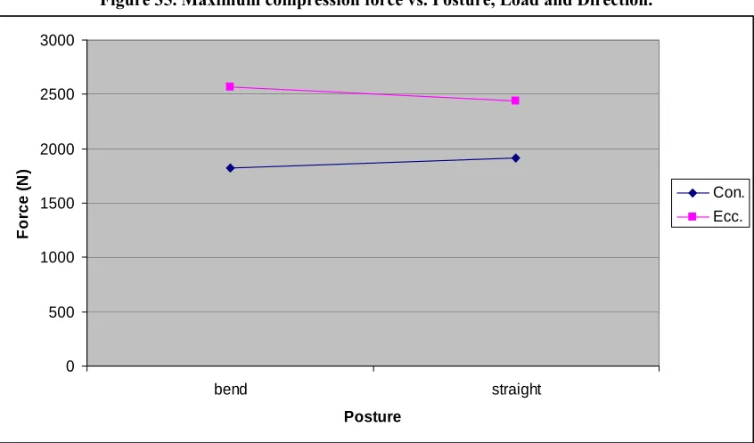
(3680N vs. 3114N in experiment one, and 2516N vs. 1870N in experiment two, respectively).
The variability of the spinal load in these two types of exertions was also compared in terms
of the average absolute deviation from the median (AADM) of the compression values
(where the median refers to the median values of the multiple repetitions of the same task).
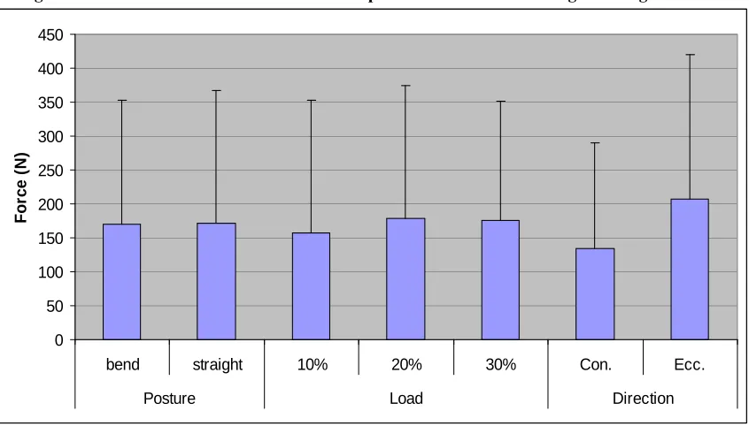
This AADM of the maximum compression force was 281N for concentric versus 472N for
eccentric exertions in experiment one, and 134N for concentric versus 207N for eccentric
exertions in experiment two. These differences were shown to be affected by the
lifting/lowering velocity, knee posture and load levels. This result has significant meaning
when considering the relative risk of lifting and lowering exertions in the workplace.
This study demonstrated an innovative method to quantitatively include the effects of
the importance of involving these passive components in the estimation of the spinal load at
the full flexed posture and eccentric exertions. The results of this study have also provided
some insight into the relative risk of eccentric vs. concentric exertions by understanding the
Biomechanical Analysis of
Eccentric and Concentric
Lifting Exertions
by
Yu Shu
A dissertation submitted to the Graduate Faculty of
North Carolina State University
in partial fulfillment of the requirements for
the Degree of Doctor of Philosophy
Industrial and Systems Engineering
Raleigh, NC
2007
APPROVED BY:
____________________ ____________________ Simon M. Hsiang Gregory D. Buckner
____________________ ____________________ David B. Kaber Gary A. Mirka
DEDICATION
BIOGRAPHY
Yu Shu was born in Sichuan province, China. After graduating from Tshinghua
University in Beijing with a Bachelor’s degree in Industrial Engineering, he joined the
Ergonomics Laboratory in the Edward P. Fitts Department of Industrial and Systems
Engineering in North Carolina State University. He worked as a research assistant under the
direction of Dr. Gary A. Mirka. He received his Master’s degree in 2005 and continued to
pursue his PhD degree in NCSU. His research areas included spine biomechanics,
electromyography, biomechanical modeling, and ergonomic intervention effectiveness
ACKNOWLEDGEMENTS
I would like to thank Dr. Gary Mirka, my advisor and mentor, for his invaluable
counsel and advice for the last five years, and my committee members: Dr. David Kaber, Dr.
Simon Hsiang and Dr. Gregory Buckner for their academic support and counsel.
I would like to acknowledge many graduate students during my Master and Doctoral
degrees for their assistance and support. I would like to thank the subjects who voluntarily
participated in my studies. I would like to thank my friends who shared their life and joy with
TABLE OF CONTENTS
List of Figures... ix
List of Tables ... xiv
1 A brief introduction... 1
1.1 Ergonomics ... 1
1.2 Epidemiology of low back disorders ... 1
1.3 Low back disorder risk factors... 2
1.4 Spinal biomechanical models ... 3
1.5 Improving biomechanical models with passive components... 4
1.6 Passive components in eccentric muscle contractions... 5
1.7 The purpose of this research ... 7
2 Literature review... 8
2.1 Biomechanics of the low back ... 8
2.1.1 Basic anatomy of the low back ... 8
2.1.2 Failure and injury of the low back ... 9
2.2 Muscle contractions: eccentric versus concentric... 11
2.2.1 Differences in force generation capacity ... 12
2.2.2 Differences in EMG activities and training ... 13
2.2.3 Differences in nervous control strategy ... 14
2.2.4 Differences in force-velocity relationship ... 16
2.2.5 Differences in variability ... 17
2.3.1 Early physical models ... 19
2.3.2 Optimization models... 21
2.3.3 EMG driven biomechanical models... 22
2.3.4 Models with eccentric motions ... 30
2.3.5 Models with passive components ... 33
3 Pilot work... 41
3.1 Subjects... 41
3.2 Apparatus ... 42
3.3 Independent variables ... 42
3.4 Dependent variables... 43
3.5 Experimental procedures ... 43
3.6 Data processing... 45
3.7 Data analysis ... 45
3.8 Results... 46
4 Model development ... 50
4.1 Input data ... 51
4.2 External moment calculation ... 52
4.3 Internal moment calculation ... 54
4.3.1 Calculating the moment from the passive components ... 55
4.3.2 Calculating the moment from the active muscles... 57
5 Experimental method ... 67
5.1 Summary of literature review ... 67
5.2.1 Subjects... 68
5.2.2 Equipment ... 69
5.2.3 Experimental design... 70
5.2.4 Procedure ... 71
5.2.5 Data processing... 73
5.2.6 Model evaluation ... 75
5.2.7 Statistical analysis... 76
5.3 Experiment two: free lifting/lowering study... 77
5.3.1 Subjects... 78
5.3.2 Equipment ... 78
5.3.3 Experimental design... 80
5.3.4 Procedure ... 81
5.3.5 Data Processing... 83
5.3.6 Model evaluation ... 84
5.3.7 Statistical analysis... 85
6 Results... 87
6.1 Experiment one: dynamometer study ... 87
6.1.1 Model Evaluation... 87
6.1.2 Comparison of eccentric versus concentric exertions... 93
6.2 Experiment two: free lifting/lowering study... 102
6.2.1 Model evaluation ... 102
6.2.2 Comparison of eccentric versus concentric exertions... 104
7.1 Assessment of the model ... 113
7.2 Comparison of eccentric and concentric exertions ... 123
7.3 Limitations of this study ... 129
8 Conclusion ... 131
References... 133
Appendix... 142
Appendix A: Matlab code... 143
LIST OF FIGURES
Figure 1. Lines of action of major trunk muscles (from Marras and Granata, 1995)... 29
Figure 2. Empirical length-strength and force-velocity modulations from Davis (1998) ... 30
Figure 3. Nonlinear stress-strain curves of spinal ligaments (from Shin, 2005) ... 38
Figure 4. Measured muscle force verses model predicted muscle force in different tasks
(from Shin, 2005)... 39
Figure 5. Normalized EMG of lumbar extensors vs. knee angle and trunk angle (50% MVC)
... 47
Figure 6. Normalized EMG of erector spinae muscle vs. flexibility and trunk angle (50%
MVC condition) (group 1 : high-flexible, group 2 : mid-flexible, group 3 : low-flexible) .... 47
Figure 7. Normalized EMG of lumbar extensors vs. knee angle, trunk angle, and flexibility
(50% MVC condition) ... 48
Figure 8. Model predicted L5/S1 joint compression force and torque from muscles vs.
flexibility... 49
Figure 9. Inputs and flow of the model... 51
Figure 10. Illustration of the 3D surface of passive moment vs. load and lumbar flexion angle
... 56
Figure 11. Illustration of the range of trunk motion in previous models and current study ... 67
Figure 12. Controlled flexion/extension exertions in ARF... 72
Figure 13. Motion sensors placed on the back of the subject ... 79
Figure 14. A dynamic lifting exertion at full flexion posture... 83
Figure 15. Mean and standard deviation of the maximum muscle stress value versus trunk
Figure 16. Measured and model predicted moment at 45° trunk flexion angle in controlled
static exertion. ... 89
Figure 17. Measured and model predicted moment at medium trunk flexion angle in controlled static exertion... 90
Figure 18. Measured and model predicted moment at full trunk flexion angle in controlled static exertion. ... 90
Figure 19. External and internal moment in controlled dynamic exertion on dynamometer. 92 Figure 20. Maximum spinal compression force vs. Load, Velocity and Direction... 95
Figure 21. Interaction between Load and Velocity on maximum compression force. ... 95
Figure 22. Maximum spinal compression force in dynamic controlled trials. ... 96
Figure 23. Maximum spinal shear force vs. Load, Velocity and Direction... 96
Figure 24. Interaction between Load and Velocity on maximum spinal shear force. ... 97
Figure 25. Maximum spinal shear force in dynamic controlled trials. ... 97
Figure 26. Median deviation of the maximum compression force in controlled dynamic exertions... 99
Figure 27. Median deviation of the maximum compression force. ... 99
Figure 28. Interaction between Load and speed on median deviation of the maximum compression force. ... 100
Figure 29. Median deviation of the maximum shear force in controlled dynamic exertions. ... 100
Figure 30. Maximum spinal shear force vs. Load, Velocity and Direction... 101
Figure 32. Interaction between Load and Direction on the median deviation of the maximum
shear force... 102
Figure 33. Measured external moment and model predicted internal moment in free lifting/lowering exertions... 103
Figure 34. Maximum spinal compression force in free lifting/lowering exertions. ... 105
Figure 35. Maximum compression force vs. Posture, Load and Direction. ... 106
Figure 36. Interaction between Posture and Direction on maximum compression force... 106
Figure 37. Maximum spinal shear force in free lifting/lowering exertions. ... 107
Figure 38. Maximum spinal shear force vs. Posture, Load and Direction... 107
Figure 39. Interaction between Posture and Direction on the maximum shear force... 108
Figure 40. Median deviation of maximum compression force in free lifting/lowering exertions... 109
Figure 41. Median deviation of maximum compression force vs. Posture, Load and Direction. ... 109
Figure 42. Interaction between Load and Direction on the maximum compression force... 110
Figure 43. Median deviation of maximum shear force in free lifting/lowering exertions.... 111
Figure 44. Median deviation of maximum shear force vs. Posture, Load and Direction. .... 111
Figure 45. Interaction of Load and Direction on median deviation of the maximum shear force. ... 112
Figure 46. Normal probability plot of the residuals of the original maximum shear force .. 150
Figure 47. Normal probability plot of the residuals of the log transformed maximum shear force ... 151
Figure 49. Residuals vs. predicted values of log transformed maximum shear force data... 152
Figure 50. Normal probability plot of the residuals of the maximum compression force.... 153
Figure 51. Residuals vs. predicted values of the maximum compression force ... 153
Figure 52. Normal probability plot of the residuals of the median deviation of the peak
compression force ... 154
Figure 53. Residuals vs. predicted values of the median deviation of the maximum
compression force ... 154
Figure 54. Normal probability plot of the residuals of the median deviation of the peak shear
force ... 155
Figure 55. Residuals vs. predicted values of the median deviation of the maximum shear
force ... 155
Figure 56. Normal probability plot of the residuals of the maximum flexion/extension
velocity... 156
Figure 57. Residuals vs. predicted values of the maximum flexion/extension velocity... 156
Figure 58. Normal probability plot of the residuals of the maximum compression force.... 157
Figure 59. Residuals vs. predicted values of the maximum compression force ... 157
Figure 60. Normal probability plot of the residuals of the maximum shear force... 158
Figure 61. Residuals vs. predicted values of the maximum shear force... 158
Figure 62. Normal probability plot of the residuals of the median deviation of the peak
compression force ... 159
Figure 63. Residuals vs. predicted values of the median deviation of the maximum
Figure 64. Normal probability plot of the residuals of the median deviation of the maximum
shear force... 160
Figure 65. Residuals vs. predicted values of the median deviation of the maximum shear
LIST OF TABLES
Table 1. List of important EMG-assisted biomechanical models... 40
Table 2. Coefficients of muscle coordinates and cross-sectional areas (Marras and Granata, 1995) ... 60
Table 3. Range of maximum muscle stress values (gain) found in the literature... 66
Table 4. Anthropometric data of the subjects in experiment one ... 69
Table 5. Anthropometric data of the subjects in experiment two ... 78
Table 6. MANOVA and ANOVA results of the maximum spine reaction forces in the dynamic exertions. ... 94
Table 7. MANOVA and ANOVA results of the median deviation values... 98
Table 8. Comparison of mean absolute error and R2 values in free lifting/lowering exertions. ... 104
Table 9. MANOVA and ANOVA test results of the maximum values in free lifting/lowering exertions... 104
1 A BRIEF INTRODUCTION
1.1 Ergonomics
Ergonomics is the scientific discipline concerned with understanding the interactions
between human beings and other elements in a system in order to optimize the overall system
performance and protect the human users. The goal of ergonomics is to “design the job to fit
people” using the knowledge of human anatomical, physiological and psychological
capabilities and limitations. There are three broad domains of specialization within the
discipline of ergonomics: physical ergonomics, cognitive ergonomics and organizational
ergonomics. The focus of the current work is in the area of physical ergonomics. Physical
ergonomics includes the consideration of human anatomical, anthropometric, physiological
and biomechanical characteristics in the design of occupational activities of human beings.
Within physical ergonomics, the study of spine biomechanics is a specialized field that
focuses on reducing the risk of low back disorders (LBDs).
1.2 Epidemiology of low back disorders
LBDs are a world-wide health problem and the most common and costly
musculoskeletal disorder in the workplace (Marras 2000; Lahiri, Markkanen et al. 2005). The
prevalence of LBDs is estimated to be between 10% and 80%, depending on the population
(Verhaak, Kerssens et al. 1998; Gilgil, Kacar et al. 2005). Older people are not the only ones
that suffer from LBDs, a relatively large percentage of young adults (14.3%) are affected as
Statistics (BLS 2004), more workers complained of pain in the lower back region than in any
other part of the body.
LBDs generate a great economic cost to society. Workers suffer loss of income and
medical costs in addition to the physical pain and stress of LBDs. In addition, industry also
spends significant resources on direct and indirect costs related to LBDs. The direct costs
include the worker’s compensation and medical treatment costs. Indirect costs include the
extra cost for hiring temporary workers and the other costs associated with lost work days are
examples of indirect costs. The total cost for LBDs has exceeded $100 billion in the United
States (Katz 2006). As a result, preventing LBDs has become a major research topic in
ergonomics.
1.3 Low back disorder risk factors
It is generally believed that LBDs occur when the applied load exceeds the failure
tolerance of one or more of the low back tissues (McGill 1997). Six specific occupational
risk factors have been identified as being associated with LBDs: lifting and forceful
movements, static work postures, physically heavy work, frequent bending and twisting,
repetitive work, and vibration (Marras, Lavender et al. 1993). Lifting (and lowering) has
been shown as one of the most dangerous occupational activities in terms of inducing LBDs
(Bernard 1997; McGill 1997). Lifting is defined as moving or bringing something from a
lower level to a higher one and vice versa for lowering. During lifting/lowering, the posterior
erector spinae muscles generate the torque to support and extend the trunk. The spine, acting
as the fulcrum of this mechanical system, must withstand not only the forces from gravity
acting on the load and the body segments, but also more significantly, the muscle forces
flexion angle increases during lowering with the maximum moment occurring near the fully
flexed posture. The full flexed posture is often seen in industries such as agriculture and
construction, and this is generally considered as a risk factor that can cause LBDs (McGill,
1997). Many tasks in the agriculture and construction industries require this posture when
farmers and construction workers manipulate objects at ground level. These industries are
noted for their high levels of low back injury/illness, e.g. vegetable farming in agricultural
production (Incidence Rate (IR) of back injury or illness = 36.2 cases per 10,000 full-time
workers), and construction field (IR = 40.2). These jobs require substantial time spent in full
or near full flexed postures and report higher incidence rates of LBDs compared to average
industry (IR of private industry of back injury or illness = 27.1) (BLS 2006).
1.4 Spinal biomechanical models
Over the years, a number of spinal biomechanical models have been developed to
quantitatively study the loading on the spine caused by various lifting activities. The purpose
of using a spinal biomechanical model is to provide a representation of the spine that can be
quantitatively analyzed and understood. For example, the compression force between two
vertebrae of spine is hard to measure in a living human body, but it can be estimated with the
help of the spinal biomechanical models. Recent biomechanical spinal models utilize a
three-dimensional multi-vector system where the major trunk muscles are modeled as single
force vectors. These force vectors counter the external moments to satisfy the static
equilibrium during isometric holding exertions and the dynamic equilibrium during dynamic
lifting motions (e.g. Marras and Granata 1995; Davis and Mirka 2000).
Accurate estimates of muscle forces are important in biomechanical models. However,
assessment is necessary. Electromyography (EMG) has been established as the most widely
used bioinstrumentation method for estimating muscular forces (DeLuca 1997). The
theoretical foundation is the EMG-force relationship, which has been investigated and
validated in the literature (Perry-Rana, Housh et al. 2003). Briefly, during muscle
contraction a motor unit action potential is created as the motor neuron initiates the muscle
contraction and ions flow into and out of a muscle cell. Surface electrodes can be placed on
the skin over the muscle to measure this electrical activity. As more force is generated by the
muscle more electrical activity can be measured. Using information with regard to the
cross-sectional area of the muscle, the maximum muscle stress (force-generating capacity per unit
cross-sectional area), and the muscle activation level measured using EMG technology in
vivo, the magnitude of the force for a specific muscle in living body can be estimated and
used in the spinal biomechanical models.
1.5 Improving biomechanical models with passive components
The EMG based biomechanical models depend heavily on the measured EMG
activities of trunk muscles. However, previous research has shown that the posterior trunk
muscles show near zero activity when one bends to full flexed posture. (Colloca and Hinrichs
2005) This is called the “flexion-relaxation phenomenon” (FRP). During the FRP, the
myoelectrical silence of muscles makes it difficult to use EMG based biomechanical models.
Consequently, the effects of the passive components including the elastic proportions
of the muscles, ligaments and disc should be considered in generating the restorative
moments in a full trunk flexion posture. McGill and Kippers (1994) confirmed that the spinal
ligaments generated the majority of the restorative moment during the FRP. It is reasonable
flexion angle decreases, while the restorative moment from active muscles will increase and
finally take the role of supporting the trunk. However, this interplay between the passive and
active components of the trunk has not been fully explored in the literature.
1.6 Passive components in eccentric muscle contractions
The passive component of the restorative moment is important during eccentric
contractions. Eccentric contractions are defined as contractions wherein a muscle lengthens
as it is generating muscle force, as would be seen in the biceps brachii muscle when a person
is lowering the load. For multiple muscles system such as trunk muscles, the eccentric
contractions are often described as exhibiting a negative correlation between the joint torque
and joint velocity. On the other hand, concentric contractions are contractions where the
muscle is shortening as it is generating force, as would be seen in the biceps brachii muscle
when that same person is lifting a load by flexing the elbow. They can also be defined as the
positive correlation between the joint torque and joint velocity. Research has shown that the
mechanical properties of a muscle during eccentric contractions are different from the
mechanical properties of a muscle during concentric contractions. One major difference is
that muscles are able to generate greater force during eccentric contractions than during
concentric contractions (Huang and Thorstensson 2000; Fang, Siemionow et al. 2004). It has
been hypothesized that the passive components in muscles may provide the extra tension
force during eccentric contractions (Proske and Morgan 2001). Similarly, eccentric
contractions generate more force as compared to concentric contractions at the same EMG
activation level (Huang and Thorstensson 2000). In other words, to provide the same amount
of force, a muscle generates less EMG activity in an eccentric contraction than in a
Grabiner and Owings 2002). When using the EMG signals as inputs for a spinal
biomechanical model, this important difference between the eccentric and concentric
contractions must be considered (Davis, Marras et al. 1998).
Eccentric contractions have also been found to be more variable than concentric
contractions (Fang, Siemionow et al. 2001; Christou and Carlton 2002). Christou and
Carlton (2002) found that when the subjects were asked to reach the same knee-extension
torque in both eccentric and concentric exertions, the standard deviation of the forces
generated in the eccentric contractions was larger than those in the concentric contractions. In
another study, Fang, Siemionow et al (2001) found that controlled eccentric motions were
more difficult to perform because of higher force fluctuations as compared to controlled
concentric motions (Fang, Siemionow et al. 2001).
From the injury prevention standpoint, eccentric contractions have been found to be
more likely to cause injury than concentric contractions. For a given level of force production,
eccentric contractions cause more damage to the myotendinous tissues, as compared to
concentric movements, because muscle fibers are forced to elongate when contracting
(Friden, Sjostrom et al. 1983; Newham, Mills et al. 1983; Newham 1988; Shellock,
Fukunaga et al. 1991; Proske and Morgan 2001). Clinical reports suggest that hamstring
injuries occur most often as a result eccentric contractions (Sallay, Friedman et al. 1996). It is
important to note that most of the biomechanical models that have been developed to
quantify risk of injury during strenuous manual materials handling tasks have focused on
concentric contractions (i.e. lifting activities), while there are many lowering tasks (i.e.
eccentric contractions) performed every day by material handlers(McGill and Norman 1986;
reported that lowering exertions represented 15% of all kinds of exertions (lifting, lowering,
pushing, pivoting and turning, etc.) performed by 31 handlers in a warehouse. When only
considering the exertions that require vertical displacement of the load (lifting and lowering),
then 37% of these exertions were actually eccentric contractions. Understanding the risks
posed by these eccentric contractions is the focus of this study.
1.7 The purpose of this research
The focus of this research is to develop an EMG-assisted biomechanical model that
can accurately predict the spinal load from active muscles and passive components. This
model will allow for a demonstration of the transfer of the trunk support mechanism between
active muscles and passive components during the lifting/lowering trunk exertions
throughout a full range of trunk flexion, including near full flexion angle.
After that, this model will be used to explore the difference in the magnitude and
variability of the L5/S1 joint reaction forces between the eccentric (lowering) and concentric
(lifting) motions in the full range (stand straight to full flexion) of lifting and lowering
exertions. Several occupational lifting factors are considered in this study: lifting direction
(concentric vs. eccentric exertions), load weight, and lifting posture (bent or straight knee).
The results of this study will generate quantitative information about the biomechanical
loading during dynamic trunk eccentric and concentric motions and will provide additional
2 LITERATURE REVIEW
2.1 Biomechanics of the low back
2.1.1 Basic anatomy of the low back
The spine consists of seven cervical vertebrae, twelve thoracic vertebrae, five lumbar
vertebrae, five fused sacral vertebrae, and three to four fused coccygeal segments. The focus
of this study is the lumbar spine. A lumbar vertebra consists of an anterior block of bone, the
vertebral body, and a posterior bony ring, known as the neural arch, containing articular,
transverse and spinous processes. Between the vertebral bodies are intervertebral discs that
withstand compression loads and limit intervertebral motion. Around the vertebra and
between the posterior processes are ligaments that provide additional tensile resistance to
intervertebral motion. The relative movements of the vertebral bones are well-defined and
limited by these passive structures. In terms of their relative contribution to the extensor
moment during lifting, these passive tissues contribute very little in typical lifting motions
(McGill and Norman 1986) but do contribute to a greater degree in full trunk flexion
conditions (McGill and Kippers 1994).
Under normal lifting conditions, the forces generated by the trunk extensor
musculature contribute the majority of the trunk extension moment. The major muscles that
contribute to the extension of the spine are the erector spinae muscles (iliocostalis,
longissimus and spinalis) and the latissimus dorsi. The major muscles that contribute to the
flexion of the spine are the rectus abdominis, external oblique and internal oblique. When the
lifting activities the activation of the flexor muscles is often seen and is believed to provide
stability to the biomechanical system. These five pairs of muscles (left and right erector
spinae, latissimus dorsi, rectus abdominis, external and internal obliques) are included in the
majority of the spinal biomechanical models.
Under specific lifting conditions, such as picking out an item from a deep container at
ground level, the near full trunk flexion posture is often used. In this posture, the elastic force
from elongated muscles can generate a large amount of the moment to maintain the spine.
The passive components of the spine, such as ligaments and disc also function as the prime
contributors to support the spine. Sometimes, the moment from elastic muscle forces and
passive components is large enough that it is unnecessary for the nervous system to activate
muscles. In this case, myoelectric silence can be observed in the erector spinae muscles,
which is called “flexion-relaxation phenomenon”.
2.1.2 Failure and injury of the low back
Low back injury can take place in any of the tissues listed above and the degree to
which these tissues are able to heal will determine whether the damage creates an acute or
chronic injury. The majority of low back pain comes from injury to the muscles and
ligaments. The cause could be the repetitive tissue micro-trauma or a single acute trauma and
inflammation, edema and pain are the result. Fortunately, these tissues are able to heal
relatively quickly. In muscle tissue, tears are called muscle strains, while in the ligaments,
tears are called ligament sprains.
Injury to the intervertebral discs is much more problematic in that the healing
capabilities of these tissues are quite limited. Damage to the intervertebral disc can lead to
biomechanical models concentrate on quantifying the loading of these structures. The L5/S1
joint of the spine (and intervertebral disc) is the focus of the majority of biomechanical
models for lifting, holding and other industrial tasks because it is at the site of the greatest
force concentration—the base of the spine. There are three kinds of loads that occur on this
joint: compression, torsion, and shear.
Understanding the ultimate strength limits of the intervertebral discs can be an
important component to establishing safe lifting limits and is an area of considerable research.
It is impractical and unsafe to measure the maximum strength limits within a living human
subject. Most researchers in this area gather measurements in vitro on cadavers. Jager and
Luttmann (1989) reported that the mean of the compression strength limit for the spine
components was 4.36kN with a standard deviation of 1.88kN. For its updated 1991 lifting
equation, NIOSH concluded that a maximum safe compressive strength limit of 3.4kN is
appropriate for the L5/S1 intervertebral disc (Waters, Putz-Anderson et al. 1993). The
maximum torsion and shear strength for the thoracic and lumbar spine were reported to be
150N and 1800N, respectively (White and Panjabi 1990 p.9). Berkson et al. (1979)
illustrated the importance of the support of the posterior elements and ligamentous structure
of the spine in addressing the shear loads on the spine. The most significant finding was that
with a constant 400N compressive and 145N shear load applied separately toward anterior,
posterior and lateral directions, the lumbar disc displacements were approximately 50 percent
larger (0.085cm vs. 0.121cm) during posterior shear than during anterior shear with the
posterior elements intact. However, the lumber disc displacements were approximately the
same (0.124cm vs. 0.142cm) for anterior and posterior shear load when the posterior
primarily by the posterior elements (facet joints in the lumbar spine). It is important to note
that the results from in vitro studies should be used with caution because the mechanical
properties of the intervertebral disc in vivo may be significantly different from those in vitro.
For instance, Keller et al. (1990) found significant differences between the in vivo
mechanical creep behaviors of animals’ lumbar vertebrae compared to those seen in vitro.
2.2 Muscle contractions: eccentric versus concentric
According to the cross-bridge theory of muscle contraction, force is generated by the
interaction of actin and myosin filaments in the muscle fibers (cells). In concentric
contraction motion, these filaments interact and slide so that the degree of overlap of the
filaments increases, which causes the entire muscle to shorten and creates the movement.
During eccentric contractions force is generated in the same way (cyclical interaction
between the cross bridges), but the force generated is not sufficient to overcome the external
force and therefore the muscle lengthens as it is exerting force. Because the bonds between
these filaments are disrupted by the mechanical movement of the fibers as the muscle
lengthens, damage is more likely to occur in eccentric motions (Proske and Morgan 2001).
The abnormalities in the muscle fibers that have been observed after eccentric motion include
sarcolemmal disruption, distortion of myofibrillar components, lesions of the plasma
membranes, etc (Friden, Sjostrom et al. 1983; Friden and Lieber 1992; Enoka 1996). It is
also hypothesized that the dead fibers which decompose in the hours after excessive eccentric
exercise leave one feeling stiff and sore (Proske and Morgan 2001). In addition to the
difference in movement direction, there are many other differences between eccentric and
force-velocity relationship, control strategy employed by the central nervous system and variability
in performance.
2.2.1 Differences in force generation capacity
Research has consistently shown that maximum eccentric motions produce more
force than maximum concentric motions. Fang et al. (2004) found that the force exerted by
the elbow flexor muscles of the subjects during eccentric maximum voluntary contraction
exertions (210.63N) was significantly higher than the force during concentric exertions
(184.06N). In a study of trunk muscle strength in eccentric and concentric lateral flexion,
Huang and Thorstensson (2000) found that the lateral flexion torque was always higher in
eccentric than in concentric actions (211 to 218Nm vs. 66 to 140Nm). Similar results were
found by Westing et al. (1990) in the study of electrical stimulation on eccentric and
concentric torque-velocity relationships during knee extensions. Nine subjects performed
maximal voluntary, electrically evoked and superimposed eccentric and concentric knee
extensions at velocities of 60, 180 and 360°/s. The torque outputs measured at 60° for the
three eccentric contraction conditions (about 220 to 350Nm) were significantly higher than
those in concentric conditions (about 150 to 190Nm). Another important finding in this study
was that the superimposed eccentric torque was on average 21-24% greater, and electrically
evoked eccentric torques were 11-12% greater than the corresponding maximal voluntary
torques. This indicated that eccentric knee extension torque in maximal voluntary conditions
does not represent the maximal torque producing capacity. The authors proposed a neural
inhibitory mechanism to explain this finding: the neural system prevents real maximum
tension during the maximum voluntary eccentric contractions because of the risk of damage
2.2.2 Differences in EMG activities and training
Using EMG technology, researchers have found significant difference between
eccentric and concentric motions in terms of EMG activities. Generally, if the output force
generated by the muscles is the same, then eccentric motions have less EMG activity as
compared to concentric motions (Tesch, Dudley et al. 1990; Huang and Thorstensson 2000).
Aagaard et al. (2000) did a study in which the EMG activities of three knee extensor muscles
were measured before and after 14 weeks of heavy resistance training. Two levels of speed
(30 and 40°/s) were tested for eccentric and concentric motions. The EMG activities for these
pre-training muscles were 17-36% lower in eccentric motions than concentric motions. After
the heavy resistance training, the eccentric strength increased 15%-17% while the concentric
strength increased 8%-15%. The EMG activities for after-training muscles in eccentric
motions were still lower (16%-22% less) than those in concentric motions. Similar results
were found by Tesch et al. (1990). They studied the force and EMG signal patterns in
concentric and eccentric actions of knee extensor muscles. Fourteen subjects performed
unilateral, maximal voluntary concentric or eccentric quadriceps muscles actions on separate
days. The results showed that the torque in eccentric actions were greater than in concentric
actions (about 175Nm to 225Nm vs. 75Nm to 150Nm). The eccentric torque did not decline
throughout the experiment time, while concentric torque markedly decreased with time.
Though the torque was larger in eccentric actions, the integrated EMG signal was smaller as
compared to concentric actions. Thus, the ratio of integrated EMG/torque was twofold
greater at the beginning, and fivefold greater at the end for concentric than eccentric muscle
actions. These results indicated that additional force during eccentric actions must be
The authors noted that the elastic components of the muscle tissue contributed to the
additional force production during the eccentric contractions.
2.2.3 Differences in nervous control strategy
It has been suggested that the nervous control system (NCS) uses a simple, consistent
strategy to control muscle force: the NCS grades the external force and controls the muscle to
generate greater, equal or less force as compared to the external force to induce concentric,
isometric, or eccentric motions separately. However, this idea has been challenged by the
evidence found in experiments that study maximum voluntary contractions (MVC) and the
initial EMG right before both type of contractions. Fang et al. (2001; 2004) reported that the
NCS signals for eccentric actions differ from those for concentric actions. In 2001, Fang et al.
measured the electroencephalography-derived movement-related cortical potential (MRCP)
and EMG signals when eight subjects performed eccentric and concentric actions of the
elbow extensor muscles. The same amount of load (10% of the subject body weight) was
applied to the left hand of the subject during these two types of contractions. It was found
that the negative potential values of the MRCP, which are related to cortical activities for
movement preparation and execution, were greater during eccentric than concentric tasks.
The positive potential values of the MRCP, which are associated with the processing of the
feedback signals, were also greater during eccentric than concentric actions. These results
indicated that the brain plans for eccentric movements differently that it does for concentric
movements. In 2004, Fang et al. did a similar study in which the subjects performed
maximum voluntary eccentric and concentric contractions of elbow flexor muscles.
Two-dimensional mapping of MRCP was measured to examine the spatial and temporal
differences occurred in both temporal and spatial distributions, which suggest that “cortical
activation patterns between the controlling processes of eccentric and concentric movements
are not the same” (p.206). The number of activation areas determined by number of
electroencephalogram electrodes passing a threshold was larger at all time points in eccentric
muscle activities than in concentric ones. The patterns of activation areas in eccentric
contractions were almost completely different from those in concentric contractions.
There is other evidence to support the different control strategies between eccentric
and concentric contractions. Grabiner and Owings (2002) did some experiments studying the
EMG of the knee extensor muscles. In one experiment, when the subject performed a normal
sub maximal eccentric contraction, the EMG during the eccentric contraction averaged 84%
of the value for the concentric contraction at the same force level. However, when the
subject performed an unexpected sub maximal eccentric contraction - the subject expected to
perform a concentric contraction while the device actually forced an eccentric contraction -
the magnitude of the initial EMG for the unexpected eccentric contraction averaged 104% of
the concentric contraction. In another experiment reported in the same article, the EMG
activities of knee extensor muscles during isometric periods preceding both concentric and
eccentric exertions were evaluated. The results of this study showed that the EMG of these
muscles preceding eccentric contractions was 13% to 25% lower in the eccentric contractions
as compared to those preceding concentric contractions, again indicating a differential
“preparation” between the two types of exertions. This empirical evidence revealed that the
2.2.4 Differences in force-velocity relationship
Just as the mechanism and control strategy are different for eccentric and concentric
contractions, other basic characteristics of muscle function vary between eccentric and
concentric exertions. The most obvious difference is in the force-velocity relationship. Early
research showed that as velocity of shortening (concentric contractions) increased, the force
producing capability decreased rapidly (Wilkie 1949; Bigland and Lippold 1954). Other
studies have shown that changes in lengthening velocity (eccentric contractions) have a much
smaller impact on the force producing capability of the muscle. Huang and Thorstensson
(2000) investigated the position and velocity dependency of the torque output of lateral
flexor muscles of the trunk. The subjects in this study performed lateral eccentric and lateral
concentric isokinetic movements in the frontal plane at different lateral bending velocities
(range from -60°/s to 60°/s) were tested. The lateral trunk flexor torque in eccentric
movements was not affected by velocity, but in concentric movements, the lateral trunk
flexor torque decrease as velocity increased. Similar results were found for trunk flexion in
the sagittal plane, the trunk flexor torque decreased as the sagittal extension speed increased
(Raschke and Chaffin 1996). Sutarno and McGill (1995) did a thorough investigation of the
behavior of the erector spinae muscles in iso-velocity motions. Ten subjects performed
sagittally symmetric flexion and extension motions while the EMG of the erector spinae
muscles and the kinematics of the trunk were measured. The lower erector spinae muscles
(L3 level) followed the typical force-velocity relationship. During the eccentric exertions, the
muscle force remained at approximately 1.3 times that of the maximum force under isometric
conditions, while the muscle force decreased when the velocity of the concentric contractions
2.2.5 Differences in variability
There have been a number of studies that have shown differences in measures of
variability of biomechanical performance when comparing eccentric and concentric exertions.
In a study of elbow flexor muscles, Fang et al. (2001) reported greater force fluctuations
during controlled sub-maximal eccentric contractions as compared to concentric exertions.
The same amount of load was applied to the forearm of the subject when the subject
performed simple elbow flexion/extension activities. The actual dynamic force was measured
by a transducer attached to the load. The results showed that the standard deviation of the
force measured in eccentric contractions was significantly larger than that in concentric
contractions. (1.14N vs. 0.76N). In their study of maximum voluntary elbow flexion
exertions, Fang et al. (2004) considered the standard deviation of the mean force value for
the first and last of three trials for both eccentric and concentric tasks. Eccentric tasks had
significantly higher standard deviation than concentric tasks (34.15N vs. 21.80N). It was
explained by the authors that this difference in variability may be related to periodic stretch
reflex-reduced EMG bursts and elective recruitment of larger-size motor unit for eccentric
contractions. In a study of knee extension exertions, Christou and Carlton (2002) found that
motor unit output was more variable in eccentric contractions as compared with concentric
contractions. Ten subjects performed concentric and eccentric knee extension tasks while the
torque generated by the knee extensor muscles was measured by an isokinetic dynamometer.
Five absolute target force levels were given (50, 100, 150, 200 and 250N) and the subjects
were asked to reach the target force level when performing eccentric or concentric motions at
an angular velocity of 50°/s. Concentric motions started from 90° and moved to 110° knee
knee angle. The results showed that mean force value at each target level was not
significantly different between eccentric and concentric motions, but the standard deviation
and coefficient of variation of peak force were larger in the eccentric than concentric
exertions. Furthermore, the variability of the time to reach peak force was also greater for
eccentric motions. It is believed that these differences in variability reflect differences in
control strategy/capability and this most likely due to differences in the relative contribution
of the passive component of the muscle force found in the eccentric exertions. As introduced
before, the difference in nervous control strategy may also contribute to the difference in the
variability of force production between eccentric and concentric contractions.
2.3 Biomechanical models of the spine
As described in the Introduction, spinal biomechanical models can be used to
quantitatively analyze the reaction forces and moments on the spine. The general steps of
developing a spinal model are as follows:
1) Establish a boundary and identify the components in this model, i.e., muscles,
ligaments, and bones, and coordinate the axes.
2) Consider the effects of gravity on the body parts and other external loads (i.e.,
objects in hands).
3) Add the internal load (force by ligaments and muscles, etc) into this model. The
external and internal load must fit the static equilibrium (
∑
F =0, ) ifthis is a static condition (i.e., holding a load in hand or isometric lifting). If this is
a dynamic condition (i.e. lifting or lowering), then the dynamic equilibrium
( ,
∑
=I⋅α) should be used.∑
M =0Regardless of the type of condition, the internal load is important because most of the
compression force on the spine comes from the forces generated by the trunk musculature
and passive tissues. The key point here is that the moment is the product of the force times
the length of the moment arm (the distance from the force line of action to the L5/S1 joint).
The erector spinae muscles have much shorter moment arms as compared to the external load.
To generate the same amount of moment to balance the external load, the erector spinae
muscles must exert much larger forces than the gravity force of the external load alone
(McGill and Norman 1986; Mirka, Kelaher et al. 1997). With the activation of the antagonist
abdominal muscles, the forces are even greater. All these forces are internal forces that must
be resisted by the spine. Thus, with the help of the spinal biomechanical model, researchers
can take an inside view of the “real” load on the spine and have a better understanding of the
risk factors related to LBDs.
2.3.1 Early physical models
Early biomechanical modeling attempts for the lumbar spine were done by Morris, et
al. (1961). The authors used a single vector of force in the sagittal plan to represent the
erector spinae group of muscles forces. The moment arm of the back muscles related to the
fulcrum (the lower lumbar part of the spine) was two inches. In their model the force
generated by back muscles was calculated under the condition of static equilibrium. The total
external moment from the weight of the body and the load was calculated first. The internal
moment calculated as the back muscle force times the moment arm was set to be equal to the
external moment. In this condition, the only unknown variable was the back muscle force, so
on the spine could be determined (Morris, Lucas et al. 1961). This model demonstrated the
logic of calculating the spinal load from external load and muscles forces.
Later, Chaffin and colleagues (Chaffin 1969; Chaffin and Baker 1970) introduced a
static sagittal plane model that could be used to predict the capacity of hand lifting strength.
The goal of the model was to use the body anthropometry data, posture data, and maximum
voluntary articulation torques as input data to predict the lifting capacity in various postures.
First, the whole human body was divided into segments and described as seven solid links:
feet, lower legs, upper legs, trunk (with neck and head), upper arms, lower arms, and hands.
Then, the anthropometric data of the body such as body weight, stature, center of gravity of
the hand to wrist distance, and foot length, etc., were collected. The articulation angles of the
seven body parts were recorded along with the maximum voluntary torque between each pair
of connected body parts, e.g., maximum elbow flexion torque, shoulder flexion, hip
extension, knee extension and ankle planter flexion. With all these inputs, the author was
able to predict the maximum hand lifting torque at a specific position and tell which joint was
the weak point or, in other words, when a specific joint reached the maximum voluntary
torque. In addition to these predictions, the biomechanical model was also able to calculate
the moments/forces acting about/on the individual joints in the kinematic chain. To calculate
these forces in the low back, a single extensor equivalent muscle was introduced, which
generated the required force to create the necessary extensor moment. This basic approach
allowed the researcher to show how varying the lifting posture affected not only the lifting
capacity, but also the stresses on the low back.
From that point, biomechanical models were improved in two major directions: 1)
(i.e., examining multiple muscle models instead of using the single extensor equivalent;
considering the origin, insertion and line of action of the trunk muscles; considering both the
length-tension and force-velocity relationship of the trunk muscles) and 2) greater
applicability by considering more kinds of motions of the body including flexion, lateral
bending and twisting; moving from static posture to dynamic exertions; and considering
stochastic features.
2.3.2 Optimization models
The major problem with the multi-muscle biomechanical models is that the number of
muscles in the model is often larger than the number of equilibrium equations, which results
in an indeterminate system. From a biomechanical point of view, there are numerous
solutions for the activation patterns of the agonist and antagonist muscles to fit the force and
moment equilibriums during lifting activities (Mirka and Marras 1993). When only one
muscle was used to counter the external load, the calculation of the muscle force could be
done using simple algebra. As additional muscles were added, the system became statically
indeterminate and other approaches needed to be considered. One such approach was the use
of optimization through linear programming. Schultz and Andersson (1982) used this
approach to estimate the forces generated by five major bilateral trunk muscles. The
objective function of the linear programming formulation was the minimization of the
compression on the spine while the constraints were that the static equilibrium was
maintained and that all of the predicted muscle forces were within their feasible range. The
results of this study showed that the muscles with the greatest moment arm were activated up
to their maximum capacity and then other muscles were recruited. The authors pointed out
force from the abdominal muscles (not what really happens during realistic lifting tasks) and
2) there was no synergistic muscle activation of the extensor muscles (not what really
happens during realistic lifting tasks). While there have been a great number of optimization
models developed to try to overcome these challenges, none have been effective at predicting
the complex synergist/antagonist muscle coactivation patterns that are utilized in complex
three-dimensional lifting tasks.
2.3.3 EMG driven biomechanical models
Another approach that researchers have taken to try and overcome this static
indeterminacy problem is to use empirical data describing muscle co-activation patterns.
Electromyography plays a central role in this approach and these are called EMG-driven or
EMG-assisted biomechanical models.
The use of the electromyographic method to study spine muscles can be traced back
to the 1960’s. In early EMG studies like Morris et al. (1962), the EMG signals was only used
to detect the activation pattern in certain trunk motions, muscle on/off patterns, and relative
muscle activation levels. The limitation to this approach was that these EMG values could
only be compared within each individual muscle; the forces between different muscles could
not be compared. In addition, the spine load could not be estimated as no actual muscular
force was calculated. Despite these limitations, these studies did provide insightful
information about the working parameters that would affect muscle activation patterns.
More recent studies have made use of the EMG data to predict the force generated by
the individual muscles. The basic principle used in this modeling approach is that the force
exerted by a muscle can be calculated using a maximum muscle stress value (sometimes
area (e.g. 50N/cm2). The muscle activation level during a task can be expressed as a
percentage of their capacity often called the normalized EMG value. The 100% value used
in this normalization can be determined when the person performs a maximum voluntary
contraction. When the same muscle performs a normal exertion, the EMG signals measured
are normalized to the maximum EMG signal and the result is expressed in terms of a
percentage value, which can also be viewed as the percentage of maximum force generated
by that muscle. For example, if a given muscle the EMG value generated during a maximum
voluntary exertion was 2.5 volts and the EMG value for that muscle during a sub-maximal
task was 0.5 volts, then that muscle has a normalized EMG value of 20% (0.5/2.5). If from
other sources we know that the maximum muscle stress value is 50N/cm2 and the
cross-sectional area is 5 cm2 for that muscle, then the maximum muscle force which is related to
the 100% EMG activity or maximum EMG signal is determined and can be calculated as
50N/cm2 × 5 cm2 = 250N. The muscle force in the sub-maximal task for that muscle can then
be calculated as 0.2 × 250N = 50N. There are a number of other factors that need to be
considered that will be addressed later, however this is the basic technique to be followed in
the EMG-driven modeling approach.
The maximum muscle stress value (also called gain factor) is an important factor in
this equation. It can be calculated in several different ways. Some models suggest the
maximum muscle stress value could be calculated from regression based on a subject’s
anthropometry, but these are not extremely highly correlated (e.g., R2=75%) due to “reasons
not fully understood at this point” (Marras and Sommerich 1991). Some models (McGill and
Norman 1986; Reilly and Marras 1989) allow the maximum muscle stress value to vary from
satisfying the equilibrium requirement). Some models calculate the average of maximum
muscle stress value by comparing the external and internal torques from a subject’s empirical
data during a subset of experimental trials and then use that mean maximum muscle stress
value in all subsequent calculations for that specific subject (Marras and Sommerich 1991;
Marras and Granata 1995).
The most effective EMG-assisted models can be categorized into two major groups:
the McGill group and the Marras group. The first EMG-assisted model in McGill’s group
was developed by McGill and Norman in 1986. This model employed many physical
components from previous spinal biomechanical models but added the empirical EMG inputs
to drive the model. Many of the basic procedures used in this model are still used in more
recent EMG-assisted biomechanical models including this study, so a close look at some of
the details of this model is useful.
This model uses three input sources: the surface EMG for measuring EMG activities
of the trunk muscles, the trunk postural marker recorded on film providing the orientation
and motion of the trunk, and the BIOMECH model (McGill and Norman 1987) that provided
the reactive L5-L5 moment and force generated by the gravity of the body and the load in
subject’s hand. Three subjects were recruited from which source data was collected. The
subjects were asked to perform six lifting tasks at different load and lifting speed conditions.
The lifts were sagittally symmetric. The results of this model were the three dimensional
reaction forces and moments on the L4-L5 joint.
There are three major steps in the processing of this model. First, the net external
moments about L4-L5 joint are calculated through the BIOMECH model based on the
(McGill and Norman 1987). It is a fully dynamic, linked-segment, total body model that
included hands, forearms, upper arms, head-neck, thorax-abdomen, pelvis, thighs, legs and
feet segments. The film coordinate data and the forces on the hands are used as inputs and the
external L4-L5 moment and force time histories generated in lifting the loads are the outputs.
Second, the net external moment is distributed to the restorative components provided
by the disc bending, ligaments strain and active muscle contraction. The component
distributions to the discs and ligaments are determined first, because the moments generated
by these components depended only on trunk flexion angle. For example, the restorative
moment produced by the disc is calculated from an exponential regression equation with the
L4 disc flexion angle as the only variable. The remaining moment is then allocated to the
muscles. The value of the force generated by a particular muscle is calculated as the product
of normalized EMG, maximum muscle force (Po) and an error term or gain value (G), and
adjusted by the coefficient of velocity (Ω) and coefficient of length (δ). The equation is:
δ
× Ω × × ×
=normalized EMG Po G
force Muscle
In this equation, the maximum muscle force and an error term represent the maximum
muscle stress value and the muscle cross area, as noted before. The calculated muscle force is
also modified by the instantaneous velocity of shortening and length of the muscle. Generally,
the greater the velocity of shortening (concentric), the smaller the force generation capacity
for that muscle. But when the muscle is lengthening (eccentric), the force generation capacity
is a larger constant regardless of the lengthening velocity. So the force generated by the
muscle should be “discounted” at a higher shortening velocity, and “inflated” at any
⎪⎩ ⎪ ⎨ ⎧ − ≤ < < − ≥ − + − × = Ω 125 . 0 125 . 0 125 . 0 125 . 0 2 . 1 6 . 1 1 ) 9 . 0 /( ) 9 . 0 ( 25 . 0 v v v v v v
where v is the shortening/lengthening velocity relative to the resting length of that muscle.
Similar procedures were conducted to adjust the force by the length and geometric
restrictions. The force generation capacity reaches maximum when the muscle is at resting
length. The coefficient of the length is calculated as:
[
( 0.05)]
sin × −
= π l
δ
where the l is the length relative to the resting length of that muscle. The calculated net force
is applied to the three-dimensional line of action of this muscle resulting in a force vector for
that muscle. The moment generated by this muscle is a three dimensional vector, calculated
as the cross product of the force vector and the muscle origin vector. The sum of the moment
from all muscles, together with the restorative moments from the disc and ligaments, is
compared with the total external moment. To bring this system to equilibrium, a gain value is
calculated. The same gain value is used for the force calculation of all muscles in this step.
This gain value is considered as an “error” term and is adjusted at each time point so that the
total net restoration moment is the same as the net external moment in the whole lifting
procedure. It is possible for the gain value to vary as a function of time for the same subject.
Finally, the compression, shear and torsion forces are calculated as the sum of the
three-dimensional force vector generated by the muscles, disc and ligaments as well as the
external load. This model revealed that the muscular components were the dominant factors
in producing restoration moments and generated approximately 99% of the moments. The
disc and the ligaments counted for less than 1%. While this model has great advantages as
maximum stress value) was adjusted in each trial and was not consistent for the same subject,
which directly opposes the physiological indications that a muscle’s force generating
capacity is directly related to muscular cross sectional area and should be consistent for an
individual (Granata and Marras 1993); 2) the subjects were asked to maintain the flat-backed
posture, which “reduced the action of ligaments to provide joint motion constraints”. The
activation of the passive posterior ligamentous system may be significant in flexed spine
(White and Panjabi 1990; Granata and Rogers 2007) or full flexion conditions (McGill and
Kippers 1994). Another limitation was that only sagittal lifting exertions were studied in this
model. But McGill et al. expanded this model to explore axial trunk twisting motions
(McGill and Hoodless 1990) and lateral bending motions (McGill 1992).
In addition to the McGill-group models, Marras and colleagues developed another
group of EMG-assisted biomechanical models. The first model for the Marras-group was the
SIMULEFT by Reilly and Marras (1989). This was a deterministic simulation model which
described the relative changes of the spinal load based on trunk muscle EMG activities
during a sagittally symmetric trunk exertion. The obvious disadvantage of this model was
the lack of maximum muscle stress value, thus no direct calculation of muscular forces was
presented.
Later in 1991, Marras and Sommerich introduced an EMG-assisted biomechanical
model which included the maximum muscle stress value. (Marras and Sommerich 1991a;
Marras and Sommerich 1991b) The advantage of this model was the capability of estimating
the real magnitude of the trunk loading. This model suffered the same limitation as the early
McGill models in that the maximum muscle stress value was adjusted for the same subject
muscles lines of action and moment arms data were the simplified three dimensional vectors
adapted from Schultz and Andersson (1981). As the authors pointed out, this model could be
improved with more accurate estimates of the force vectors, the muscle cross-sectional areas
and the locations relative to the spine.
Granata and Marras (1993) expanded this model and conducted a new method to
calculate the maximum muscle stress value. Unlike previous EMG-assisted biomechanical
models that allowed the maximum muscle stress value to vary at each time point. This model
adjusted the maximum muscle stress value so that the average value of the measured external
torque was within 5% range of the average value of the model predicted torque. Thus, the
equilibrium of the net external and internal torques was not met at each time point but
equilibrium was met for the overall net external and internal torques. Through this method,
the authors found that the maximum muscle stress value for a given subject did not vary
significantly between the experimental trials, a result which was consistent with the
physiological conclusion that the maximum muscle stress value should be constant for the
same person.
The fixed maximum muscle stress value in this model had a significant advantage
over the McGill and the previous Marras models with varied values. Not only because it was
consistent with the physiological expectations, but also because it provided a means of
validating the models. In previous models with varied maximum muscle stress values, the
errors in the model (inaccurate position and orientation of the muscles, inappropriate
presentation of the disc and ligaments) did not affect the performance of the model since the
predicted internal torque always matched the external torque. In this model with fixed
explained by the changes in the muscles’ EMG activities and the trunk kinematics. In other
words, the predicted torque should match the external torque as much as possible. The R2
values between the external torque and model predicted torque could be used as the index of
the performance of the model. Using this method, a validation procedure was conducted by
the authors to verify the accuracy of this model. It was found that the model was able to
reliably predict trunk torque. It was capable of explaining more than 70% of the variability in
trunk torque production in most trials (Marras and Sommerich, 1991b). However, this model
still utilized sub-optimal muscle force vector data. This problem was addressed when Marras
and Granata replaced the structure with a more accurate anatomical muscle structure when
expanding this model to include trunk twisting exertions (Marras and Granata 1995). In this
model, they presented a truly three-dimensional structure of the major trunk muscles (see
Figure 1).