A Survey of Recent Trends in Multiobjective Optimal Control -- Surrogate Models, Feedback Control and Objective Reduction

A survey of recent trends in multiobjective optimal

control – surrogate models, feedback control and

objective reduction

Sebastian Peitz1,∗, and Michael Dellnitz1

1 _{Paderborn University, Warburger Str. 100, 33100 Paderborn, Germany}

* Correspondence: [email protected]

Abstract:Multiobjective optimization plays an increasingly important role in modern applications, where several criteria are often of equal importance. The task in multiobjective optimization and multiobjective optimal control is therefore to compute the set of optimal compromises (thePareto set) between the conflicting objectives. The advances in algorithms and the increasing interest in Pareto optimal solutions have led to a wide range of new applications related to optimal and feedback control which results in new challenges such as expensive models or real-time applicability. Since the Pareto set generally consists of an infinite number of solutions, the computational effort can quickly become challenging which is particularly problematic when the objectives are costly to evaluate or when a solution has to be presented very quickly. This article gives an overview over recent developments in accelerating multiobjective optimal control for complex problems where either PDE constraints are present or where a feedback behavior has to be achieved. In the first case, surrogate models yield significant speed-ups. Besides classical meta-modeling techniques for multiobjective optimization, a promising alternative for control problems is to introduce a surrogate model for the system dynamics. In the case of real-time requirements, various promising model predictive control approaches have been proposed, using either fast online solvers or offline-online decomposition. We also briefly comment on dimension reduction in many-objective optimization problems as another technique for reducing the numerical effort.

Keywords:Multiobjective Optimization; Optimal Control; Model Order Reduction; Model Predictive Control

MSC:90C29;49M37

1. Introduction

There is hardly ever a situation where only one goal is of interest at the same time. When performing a purchase for example, we want to pay a low price while getting a high quality product. In the same manner, multiple goals are present in most technical applications, maximizing quality versus minimizing the cost being only one of many examples. This dilemma leads to the field of

multiobjective optimization, where we want to optimize all relevant objectives simultaneously. However, this is obviously impossible as the above example illustrates. Generically, the different objectives contradict each other such that we are forced to choose a compromise. While we are usually satisfied with one optimal solution in the scalar valued setting, there exists in general an infinite number of

optimal compromisesin the situation where multiple objectives are present. The set of these compromise solutions is called thePareto set, the corresponding points in the objective space form thePareto front. Since the solution to a multiobjective optimization problem (MOP) is a set, it is significantly more expensive to compute than the optimum of a single objective problem, and many researchers devote their work to the development of algorithms for the efficient numerical approximation of Pareto sets. These advances have opened up new challenging application areas for multiobjective optimization. In optimal control, the optimization variable is not finite-dimensional but a rather function, typically depending on time. The goal is to steer a dynamical system in such a way that one (ore multiple)

objectives are minimized. Two particularly challenging control problems are feedback control and control problems constrained by partial differential equations (PDEs). In the first case, the time for computing the Pareto set is strictly limited, often to a small fraction of a second. In the latter case, even the solution of single objective problems is often extremely time consuming so that the development of new algorithmic ideas is necessary to make these problems computationally feasible.

In fact, in situations like these, surrogate models or dimension reduction techniques are a promising approach for significantly reducing the computational effort and thereby enabling real-time applicability. This article gives an overview over recent advances in surrogate modeling for multiobjective optimal control problems, where the approach is to replace the underlying system dynamics by a reduced order model which can be solved much faster. On the other hand, it introduces an approximation error which has to be taken into account when analyzing convergence properties. The article is structured as follows. In Section2, we are going to review some basics about multiobjective optimization, including the most popular solution methods. The two main challenges are addressed individually in the next sections, starting with expensive models in Section3. There are also surrogate modeling approaches for MOPs which directly provide a mapping from the control variable to the objective function values. Since there already exist extensive surveys for this case (cf. [1–3], for instance), these are summarized only very briefly. In Section4, real-time feedback control is discussed. Finally, we briefly discuss the question of dimension reduction in the number of objectives in Section5before concluding with a summary of further research directions in Section6.

2. Multiobjective optimization

In this section the concepts of multiobjective optimization and Pareto optimality will be introduced and some widely-used solution methods will be summarized. More detailed introductions to multiobjective optimization can be found in, e.g., [4,5].

2.1. Theory

In multiobjective optimization we want to minimize multiple objectives at the same time. Consequently, the fundamental difference to scalar optimization is that the objective function

J:U →Rkis vector-valued. Hence, the general problem is of the form

min

u∈U J(u) =minu∈U



 

J1(u)

.. .

Jk(u)



 

s.t. gi(u)≤0, i=1, . . . ,l,

hj(u) =0, j=1, . . . ,m,

(MOP)

whereu ∈ U is thecontrol variableandg : U → Rl, g(u) = (g1(u), . . . ,gl(u))> andh : U → Rm,

h(u) = (h1(u), . . . ,hm(u))>, are inequality and equality constraints, respectively. The space of the control variablesUis also called thedecision space(according to the termdecision variableforuin classical multiobjective optimization) and the objective function mapsuto theobjective space. Depending on the problem setup,Ucan either be finite-dimensional, i.e.U =Rn, or some appropriate function space.

Remark 1. It is common in finite-dimensional optimization to use the notation x for the control or optimization variable and F for the objective function. In contrast to that, u and J are more common for control problems. In order to unify the notation, the latter will be used throughout this article for all optimization and optimal control problems.

we have the system dynamics as an additional constraint, very often in the form of ordinary (ODEs) or partial differential equations (PDEs):

˙

y(x,t) =G(y(x,t),u(t)), (x,t)∈Ω×(t0,te],

a(x,t)∂y

∂n(x,t) +b(x,t)y(x,t) =c(x,t), (x,t)∈Γ×(t0,te], y(x,t0) =y0(x), x∈Ω,

(PDE)

where the domain of interestΩ ⊂ _Rnx _{is a connected open set with spatial dimensionnxand the} boundary is denoted byΓ =∂Ωwith outward normal vectorn. The coefficientsa(x,t),b(x,t)and c(x,t)in the boundary condition are given by the problem definition. The operatorGis a partial differential operator describing the evolution of the system. The cost functional ˆJ:U × Y →Rkof an optimal control problem consequently depends on the controluas well as the system statey, which results in amultiobjective optimal control problem:

min u∈U,y∈Y

ˆ

J(u,y) = min u∈U,y∈Y



  

Rte

t0 C1(y(x,t),u(t))dt+Φ1(y(x,te)) ..

.

Rte

t0 Ck(y(x,t),u(t))dt+Φk(y(x,te))



  

s.t. (PDE)

gi(y,u)≤0, i=1, . . . ,l,

hj(y,u) =0, j=1, . . . ,m.

(MOCP)

There are articles on multiobjective optimal control which specifically address the implications of multiple objectives for optimal control [6,7], see also [8] for a short survey of methods. However, for many problems there exists a unique solutionyfor everyusuch that (MOCP) can be simplified by introducing a so-calledcontrol-to-state operatorS : U → Y, see [9] for details. By setting ˆJ(u,y) =

ˆ

J(u,Su) =J(u), the problem is transformed into (MOP). For this reason, we will from now on only consider (MOP).

In the situation whereU is a function space (i.e., in the case of optimal control), the problem can be numerically transformed into a high- yet finite-dimensional problem in adirect solution method

via discretization, cf. [10,11]. This results in a large number of control variables which can be very challenging on its own in multiobjective optimization. If the system dynamics are governed by a PDE, then the spatial discretization of the stateyresults in an even higher number of unknowns which can easily reach several millions or more [12].

In contrast to single objective optimization problems, there exists no total order of the objective function values inRkwithk≥2 (unless they are not conflicting). Therefore, the comparison of values is defined in the following way [4]:

Definition 1. Let v,w∈Rk. The vector v isless thanw (denoted by v<w), if vi<wifor all i∈ {1, . . . ,k}.

The relation≤is defined in an analogous way.

A consequence of the lack of a total order is that we cannot expect to find isolated optimal points. Instead, the solution to (MOP) is the set of optimal compromises (also called thePareto setorset of non-dominated points):

Definition 2. Consider the multiobjective optimization problem(MOP). Then 1. a point u∗dominatesa point u, if J(u∗)≤J(u)and J(u∗)6= J(u).

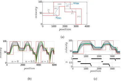
3. the set of non-dominated feasible points is called thePareto setPS, its image thePareto frontPF. A consequence of Definition2is that for each point that is contained in the Pareto set (the red line in Figure1(a)), one can only improve one objective by accepting a trade-off in at least one other objective. Figuratively speaking, in a two-dimensional problem, we are interested in finding the “lower left” boundary of the feasible set in objective space (cf. Figure1(b)).

(a)

0 5 10 15

J₁₍u₎ 0

5 10 15

J2

(

u

)

J∗

(b)

Figure 1. The red lines are the Pareto set (a) and Pareto front (b) of an exemplary multiobjective optimization problem (two paraboloids) of the form minu∈RJ(u),J:R2→R2. The pointJ

∗ _{= (0, 0)}>

is called the utopian point.

Similar to single objective optimization, a necessary condition for optimality is based on the gradients of the objective functions. The first order conditions were independently discovered by Karush in 1939 [13] and by Kuhn and Tucker in 1951 [14]. Due to this, they are widely known as the

Karush-Kuhn-Tucker (KKT)conditions:

Theorem 1([14]). Let u∗be a Pareto optimal point of problem (MOP)and assume that∇hj(u∗)for j = 1, . . . ,m, and ∇gs(u∗) for s = 1, . . . ,l, are linearly independent. Then there exist non-negative scalars

α1, . . . ,αk≥0with∑ki=1αi =1,γ∈Rmandµ∈Rlsuch that k

∑

αi∇Ji(u∗) + m

∑

γj∇hj(u∗) + l

∑

µs∇gs(u∗) =0,

hj(u∗) =0, j=1, . . . ,m,

gs(u∗)≤0, s=1, . . . ,l,

µsgs(u∗) =0, s=1, . . . ,l,

µs ≥0, s=1, . . . ,l.

(KKT)

2.2. Solution methods

Many researchers in multiobjective optimization focus their attention on developing efficient algorithms for the computation of Pareto sets. Algorithms for solving MOPs can be compiled into several fundamentally different categories of approaches. The first category is based onscalarization techniques, where ideas from single objective optimization theory are extended to the multiobjective situation. All scalarization techniques have in common that the Pareto set is approximated by a finite set of Pareto optimal points which are computed by solving scalar subproblems. Consequently, the resulting solution methods involve solving multiple optimization problems consecutively. Scalarization can be achieved by various approaches such as the weighted-sum method, thee-constraint method,

normal boundary intersection, or reference point methods [4,5,15].

Continuation methodsmake use of the fact that under certain conditions, the Pareto set is a smooth manifold of dimensionk−1 [16]. This means that one can compute the tangent space in each point of the set, and a predictor step is performed in this space. The resulting point then has to be corrected to a Pareto optimal solution using a descend method [17].

Another prominent approach is based onevolutionary algorithms[18,19], where the underlying idea is to evolve an entire population of solutions during the optimization process. Significant advances have been made concerning multiobjective evolutionary algorithms (MOEAs) in recent years [20,21] (see also [22] for a survey) such that they are nowadays the most popular choice for solving MOPs due to the applicability to very complex problems and being easy to use in a black box fashion. Since convergence rates can be relatively slow for MOEAs, they can be coupled with locally fast methods close to the Pareto set. These approaches are known asmemetic algorithms, see, e.g., [23–26].

Set-oriented methods provide an alternative deterministic approach to the solution of MOPs. Utilizing subdivision techniques, the desired Pareto set is approximated by a nested sequence of increasingly refined box coverings [27–29]. This way, a superset is computed which converges to the desired solution, even in situations where the Pareto set is disconnected. However, their complexity depends on both the dimension of the Pareto set as well as the decision space dimension. Due to this, one has to take additional steps to apply these algorithms for multiobjective optimal control problems. Depending on the method of choice, gradient information can be used to accelerate convergence. While this is widely accepted in scalar-valued optimization, this is less the case when multiple objectives are present [30]. Nonetheless, many approaches exist where gradients are exploited, for example in order to create sequences converging to single points [31–33], to compute the entire set of valid decent directions [30,34], to obtain superlinear or quadratic convergence [35,36], or in combination with evolutionary approaches (memetic algorithms) [37–41]. In many of the gradient-based methods, the descent direction for all objectives is a convex combination of the individual gradients:

q(u) = k

∑

ˆ

αi∇Ji(u). (1)

Here, ˆαis a fixed weight vector which is determined in such a way that

hq(u),∇Ji(u)i<0 ∀i=1, . . . ,k, (2)

see, e.g., [31,32]. In the unconstrained case, there exists nousatisfying (2) only ifkq(u)k=0 which implies thatuis substationary, cf. (KKT).

3. Surrogate models

The above-mentioned examples can all be described by ordinary differential equations with a finite-dimensional state spaceY. In contrast to these problems, many phenomena in physics such as mechanical strain, heat flow, electromagnetism, fluid flow or even multi-physics simulations are governed by partial differential equations. Using numerical discretization schemes for the approximation of the spatial domain (such as finite elements or finite volumes) results in a very large number of degrees of freedom and a heavy computational burden. For more complex systems (such as turbulent flows [49]), simulating the dynamics is already very costly. Consequently, optimal control of these systems is all the more challenging, and considering multiple objectives further increases the cost. Due to this reason, only few problems have been addressed directly, see, e.g., [50–53]. A method exploiting special structure in the system dynamics has been proposed in [54], and a special case of Pareto optimal solutions – namelyNash equilibria– have been computed in [55,56]1.

A very popular approach to circumvent the problem of prohibitively large computational cost is the use of surrogate models. Here, the exact objective function J(u)is replaced by a surrogate

Jr_{(u), where the superscriptrstands for reduced. In many situations, this surrogate function can} be evaluated faster by several orders of magnitude. The challenge here is to find a good trade-off between acceleration and model accuracy, and many approaches have been proposed over the past two decades.

In optimal control, there are two fundamentally different ways for model reduction. The first case – which is equivalently applicable to multiobjective optimization problems – is to directly derive a surrogate for the objective function, i.e., Jr : U →_Rk _{is constructed by polynomials, radial basis} functions or other means. In optimal control, an alternative way of reducing the computational effort is by introducing a reduced model for the system dynamics:

Jr(u) =Jˆr(u,y) =Jˆ(u,Sru),

where the reduced control-to-state operatorSr_{indicates that the model reduction is due to a surrogate} model for the system dynamics.

In both situations, we cannot expect thatJr_{(u) =J(u)holds for allu∈ U. Instead, we introduce an} error which has to be taken into account. This is closely related to questions concerning uncertainty and noise. In this context, many researchers have addressed inaccuracies. In [58], the notion ofe-efficiency

(cf. Definition3) was first introduced in order to handle uncertain objective values. Uncertainty has also been considered in the context of multiobjective evolutionary computation, see, e.g., [59–61]. Alternative methods such as probabilistic [62,63], deterministic [64] or set-oriented approaches [65,

66] have also been proposed. The special case of many-objective optimization is covered in [67], applications are addressed in [68,69]. A different approach to uncertainties is via robust algorithms. Several examples from multiobjective optimization as well as optimal control can be found in [43,70–

72].

3.1. Inaccuracies ande-dominance

When using surrogate models in order to accelerate the solution process, we have to accept an error both in the objective function as well as the respective gradients. Furthermore, inaccuracies may occur due to stochastic processes or due to unknown model parameters. In these situations, the objective function and the corresponding gradients are only known approximately which has to be taken into account.

Suppose now that we only have approximationsJr(u),∇Jr(u)of the objectives Ji(u)and the gradients∇Ji(u),i=1, . . . ,k, respectively. Furthermore, let us assume that upper boundse,κ∈Rk for these errors are known:

kJ_ir(u)−Ji(u)k2≤ei ∀u∈ U, (3) k∇Jr_i(u)− ∇Ji(u)k2≤κi ∀u∈ U. (4) In this situation, we need to replace the dominance property2by an inexact version, also known ase-dominance (see also [58,69]):

Definition 3([66]). Consider the multiobjective optimization problem(MOP)where the objective function J(u)is only known approximately according to(3). Then

1. a point u∗confidently dominatesa point u, if Jr(u∗) +e≤Jr(u)−eand Jr_i(u∗) +ei< Jir(u)−ei

for at least one i∈1, . . . ,k.

1 _{When not using a priori selection methods such as scalarization or Nash equilibria, a decision maker to select the appropriate}

solution. This is calledMulticriteria Decision Making (MCDM)[57] and is an entire area of research of its own. Thus, we will not go into further details about the decision making process here.

(a) (b)

(c) (d) (e)

2. Theset of almost non-dominated pointswhich is a superset of the Pareto setPSis defined as: P_S,e =nu∗∈ U

@u∈ Uwhich confidently dominates u

∗o

. (5)

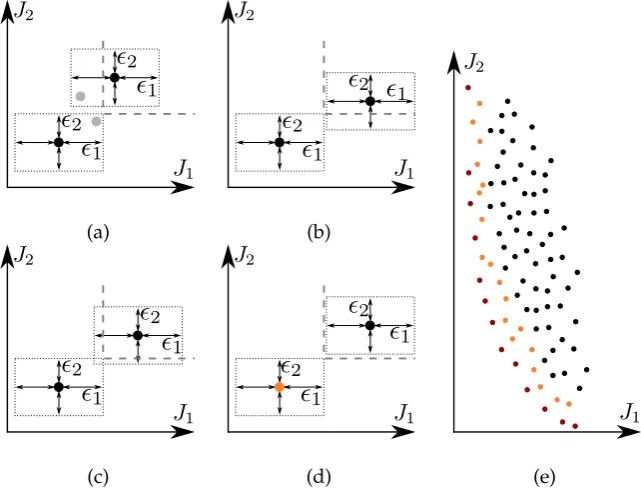
The concept ofe-dominance is visualized in Figure2. Theoretically, the true point could be

anywhere inside the box defined byesuch that in the cases (a) to (c), the lower left point does not

confidently dominate the other point. The necessary condition is violated for one component in (a) and (b), respectively, and for both components in (c). The gray points in2(a) show a possible realization of the true points in which no point is dominated by the other. In (d) the orange point confidently dominates the black one and in (e) we see the implications for the computation of Pareto fronts. Due to the inexactness, the number of points that are not confidently dominated is larger than in the exact case. This is also evident in Figure3, where the exact and the inexact solution of an example problem from production [32] have been computed with an extension of the subdivision technique presented in [27], cf. [66] for details. Here, inexactness is introduced due to uncertainties in pricing. e-dominance

can be used for the development of algorithms for MOPs with uncertainties [59,61–63,65,67,68], for accelerating expensive MOPs [60,66,73] as well as for increasing the number of compromise solutions for the decision maker [63–65,69].

When considering gradient-based methods, inaccuracies in the gradients (Equation (4)) have to be taken into account. Since only approximations of the true gradient are known, these result in an inexact descent directionqr(u). The inaccuracy in the gradients introduces an upper bound for the angle between the individual gradients∇Jr_i(u)and the descent directionqr(u). This is equivalent to a lower bound ˆαminfor the weight vector, i.e., ˆαi∈[0, 1]in Equation (1) has to be replaced by ˆαr_i ∈[αˆmin,i, 1]for

i=1, . . . ,k:

qr(u) = k

∑

ˆ

αr_i∇J_ir(u), (6)

see [66] for a detailed discussion. The additional constraint ensures that ifqr_{(u)is a descent direction} for the inexact problem, it is also a descent direction for the true problem. Furthermore, we obtain a criterion for the accuracy up to which we can computeP_S,subbased on inexact gradient information:

0 40 20

u

3

40

u₂

40 20

u₁ 20 0 0

5 10 15 20 25 30 35

(a) (b)

Theorem 2 ([66]). Consider the multiobjective optimization problem (MOP)without constraints. Only approximate gradients according to(4)are available and consequently, the descent direction is also only known approximately according to Equation(6). Assume thatkqr(u)k26=0andk∇Jir(u)k26=0for i=1, . . . ,k. Let

ˆ

αmin,i= 1 k∇J_ir(u)k2

2



  

kqr(u)k2κi− k

∑

j6=i ˆ

αj(∇Jir(u)· ∇Jir(u))



  

, i=1, . . . ,k.

Then the following statements are valid:

(a) If∑k_i=1αˆmin,i>1then there exists no direction q(u)with

hq(u),∇Ji(u)i<0 ∀i=1, . . . ,k,

i.e. no descent direction for the exact problem. (b) All points u with∑k

i=1αˆmin,i =1are contained in the set P_S,κ =

(

u∈_Rn k

∑

ˆ

αi∇Ji(u)

2≤2kκk∞

)

. (7)

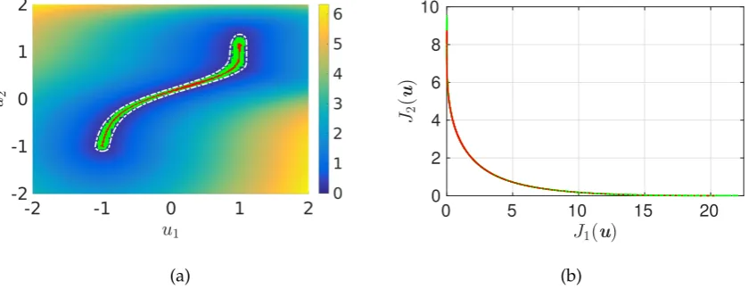
A combination of Theorem2with the subdivision algorithm from [27] is shown in Figure4. The algorithm constructs a nested sequence of increasingly refined box coverings which converges to the set of substationary points where in the unconstrained case,kq(u∗)k = 0 holds for allu∗ ∈ PS,sub.

The setP_S,subis shown in red in Figure4(a). Due to the inexactness, we can no longer guarantee kq(u∗)k =0. Instead, we obtain the setPS,κ which is shown in green. The background is colored according to the optimality conditionkq(u)kof the exact problem and the dashed white line indicates the error bound (7) from the above theorem.

(a)

0 5 10 15 20

J

u

)

0 2 4 6 8 10

J

(

u

)

Figure 4.Exact and inexact solution (P_SandP_S,κ) for a simple example withJ:R2→R2, cf. [66] for

details. (a) The setsP_SandP_S,κ(for a random error withκ= (0.01, 0.01)>) are shown in red and green, respectively. The background is colored according to the optimality conditionkq(u)kwhich has to be 0 for all substationary points. The dashed white line shows the error bound as derived in Theorem2. (b) The corresponding Pareto fronts.

3.2. Surrogate models for the objective function

is covered whereas internal states as well as the system dynamics are neglected. Using such ameta model, one can very quickly obtain the objective function value for everyu. This approach is equally applicable in finite-dimensional multiobjective optimization and has been used extensively in this context. To this end, we will only briefly cover the main questions that have to be addressed when using such models.

In special cases, one can exploit some structure in the problem formulation which yields a simplified analytic expression. However, in most cases, even if the equations can be written down in closed form, this approach requires a deep understanding of the underlying system which is often hard to get by. Moreover, small changes in the problem setup may result in having to repeat this tedious process all over. Due to these reasons, data-based approaches are used much more frequently. They are often easy to apply and much more general. In these approaches, the original objective function (or even a real-world experiment) is evaluated for a small number of inputs which are contained in the setU_ref ={u1, . . . ,up}, wherepis the number of function evaluations (orexperiments). The data pointsJ(u1_)toJ(up_{)are then used to fit the meta model such as, e.g., the coefficients of a polynomial} basis. Obviously, the choice of suitable ansatz functions is essential for the success of a meta modeling strategy. Popular choices are

• response surface models (RSM), • radial basis functions (RBF),

• statistical models such as Kriging or Gauss regression,

• machine learning methods such as Artificial Neural Networks or Support Vector Machines,

see [1] for an extensive survey in the context of multiobjective optimization. Additional surveys can be found in [74], where different statistical methods are compared, in [3,75] in relation to MOEAs, or in [76], where RSM and RBF are compared for crashworthiness problems.

Besides selecting the correct meta model, questions concerning the training data set have to be answered:

1. how large does the setUrefhave to be?

2. how can we pick the correct elements forU_ref?

3. do we defineU_refin advance or online during the model building process?

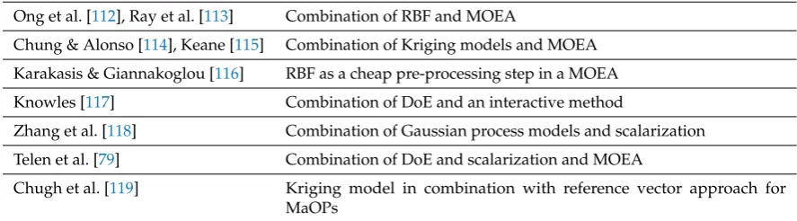
In addition to the meta model, point 1 significantly depends on the problem under consideration. The more non-linear a problem is, the more data points are generally required to accurately construct a meta model. Obviously, the number also depends on point 2, the locationsu1_touk_{of these evaluations.} The question of choosing the correct location is closely related to the field ofoptimum experimental designordesign of experiments (DoE), see, e.g., [77,78]. The relevant question there is how to optimally pick a set of experiments such that the overall approximation error becomes minimal. Such approaches have successfully been coupled with multiobjective optimization in [79,80]. Point 3 depends both on the meta modeling approach as well as the problem under consideration. In some situations (e.g., for real-world experiments), it may not be possible to iteratively determine the experiments. Instead, abatchapproach has to be used. In computer experiments, flexibility is often higher such that an interplay between model building and high-fidelity evaluations can help to further reduce the number of experiments. In the context of machine learning, this process is also known asactive learning[81,82]. Many algorithms combining multiobjective optimization and meta modeling have been proposed and there exists a vast literature concerning this topic. Table1on page17mentions both survey articles and a (non-exhaustive) selection of popular methods.

3.3. Surrogate models for the dynamical system

of the computational effort is due to solving the dynamical system, by this the reduced cost function

Jr(u) =Jˆr(u,y) =Jˆ(u,Sr_{u)is also much cheaper to evaluate.}

The use ofreduced order models (ROMs)is not limited to control but has been used successfully in a large variety of multi-query problems [12], and several extensive surveys have been written on reduced order modeling and using ROMs in prediction, uncertainty quantification or optimization, see [83–85]. For nonlinear problems, the two most widely-used approaches are thereduced basis method

andProper Orthogonal Decomposition (POD)(also known asPrincipal Component Analysis (PCA)or

Karhunen-Loève Decomposition).

3.3.1. ROMS via Proper Orthogonal Decomposition or the reduced basis method

Numerically solving a PDE is generally realized by discretizing the spatial domain with a numerical mesh using finite differences, finite elements or finite volumes. By this, the infinite-dimensional state spaceY is transformed into a finite-dimensional spaceYN _{via Galerkin} projection:

y(x,t)≈yN(x,t) = N

∑

zN_i (t)φi(x). (8)

Here,Ndenotes the number of degrees of freedom andφi(x)are basis functions with local support such as indicator functions or hat functions. This transforms the PDE into anN-dimensional ordinary differential equation for the coefficientsz. For complex domains as well as complex dynamics, the dimension can easily reach the order of millions such that solving the problem inYN _{can quickly} become very expensive which is particularly challenging in the multi-query case.

The general concept in projection-based model reduction is therefore to find an appropriate spaceYr _{with dimension` Nin which the system dynamics can nevertheless be approximated} with sufficient accuracy. The two most common approaches to do this are thereduced basis (RB) methodandProper Orthogonal Decomposition (POD). In both cases, we computesso-calledsnapshots

of the high-dimensional system and then use the data set{yN

1, . . . ,yNs }to construct a reduced basis

ψ={ψ1, . . . ,ψ`}such that

y(x,t)≈yN(x,t)≈yr(x,t) = `

∑

z`_i(t)ψi(x).

The following example describes this approach in more detail. For an extensive introduction, the reader is referred to [86,87].

Example 1(Heat equation). Suppose we want to solve the time-dependent heat equation on a domainΩwith homogeneous Neumann conditions on the boundaryΣ:

yt(x,t)−λ∆y(x,t) =0, (x,t)∈Ω×(t0,te],

y(x, 0) =y0(x), x∈Ω,

yn(x,t) =0, (x,t)∈Σ×(t0,te].

(9)

Here, y is the temperature andλis the heat conductivity. The subscripts t and n indicate the derivatives with respect to time and the outward normal vector of the boundary, respectively. We now derive the weak form of(9)

by multiplying with a test functionϕand integrating over the domainΩ. Using Gauss’s theorem, we obtain the following equation:

Z

If we want to solve(10)using the finite element method, we have to insert the Galerkin ansatz(8)into(10)

and individually take each of the basis functions as a test function. By this, we obtain the following system of equations:

Z

Ω

N

∑

zN_i,t(t)φiφj−λzNi (t)∇φi· ∇φjdx=0, j=1, . . . ,N. (11)

Introducing themass matrixM∈_RN×N_{and thestiffness matrixK∈}

RN×Nwith

Mi,j =

Z

Ωφiφjdx, Ki,j =

Z

Ω∇φi· ∇φjdx,

this yields the following N-dimensional linear system:

MztN(t)−λKzN(t) =0.

If we now want to compute a reduced order model instead of a high-dimensional finite element approximation, we can apply the same procedure except that now we have to use the reduced basis in the Galerkin ansatz as well as for test functions.

The most important difference between RB and POD is the area of application although this is not a strict separation. RB is mostly applied to parameter-dependent yet time-independent (i.e. elliptic) problems whereas POD (introduced in [88]) is applied to time-dependent problems described by parabolic or hyperbolic PDEs. Consequently, in RB the snapshots {yN

1, . . . ,yNs }are solutions corresponding to parameters{u1, . . . ,us}and in POD they are snapshots in time, collected at the time instants {t0, . . . ,ts−1}. Using an equidistant time grid h, the snapshots are taken at

{t0,t0+h. . . ,t0+ (s−1)h}. In RB, the snapshots{y₁N, . . . ,ysN}often directly serve as the basisψ.

For time-dependent problems, this can cause numerical difficulties since some snapshots might be very similar (e.g., for very slow systems or periodic dynamics) such that the snapshot matrix

S= (yN₁, . . . ,yNs )is ill-conditioned. Due to this, asingular value decompositionis performed onSand the`leading left singular vectors are taken as the basisψ. This results in an orthonormal basis which

can be shown to be optimal with respect to theL2projection error [87,88]. Furthermore, the truncation error is given by the sum over the neglected singular values:

e`= ∑ s i=`+1σi ∑s

j=1σj .

Whereas the error between the infinite-dimensional solution and the solution via a standard discretization approach can be neglected in many situations, the error of the ROM depends on several factors such as the reference data, the basis size and the parameter or control for which the ROM is evaluated. Consequently, this error can be significant such that proper care has to be taken. The most common approach is to derive bounds either for the error of the reduced statekyr−yNkor – in the case of optimal control – of the optimal solutionkur−uNkobtained using the ROM, see, e.g., [89–93] for POD or [94–97] for RB methods. In addition, there are other measures that can be taken such as deriving balanced input-output behavior [98,99] or introducing additional terms [100] or modifications [101] in the POD-based ROM. For more detailed introductions to RB and POD, the reader is referred to [97] and [87,88], respectively.

3.3.2. Optimal control using surrogate models

There is a rich literature on optimal control of PDEs using surrogate models. The approaches can be summarized in three main categories:

1. build a model once,

3. construction of regular updates using error estimators.

Whereas the first category is the most efficient one (see, e.g., [102] for optimal control of the Navier–Stokes equations), it is in general not possible to prove convergence of the resulting algorithm.

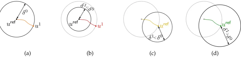
In the second approach (which was developed by Fahl [103] for POD-based ROMs and one objective), one defines a trust region within which the current surrogate model is considered as trustworthy, see Figure5for an illustration. The ROM-based optimal control problem is then solved with the additional constraint that the solution has to remain within the trust region, i.e.kui−urefk ≤δi,

whereiis the current step of the iterative optimization scheme andδiis the current trust region radius.

After having obtainedui, the high-dimensional system is evaluated and the improvement of the full system is determined:

ρ= |J

N_(ui_)−JN_(ui−1_)|

|Jr_(ui_)−Jr_(ui−1_)| .

Ifρis close to 1, then the ROM is sufficiently accurate and the iterateuiis accepted. We then use the

high-dimensional solution to construct the next ROM aturef =ui. If, on the other hand,ρis close to

0, then the ROM accuracy was bad and the iterateuiis rejected. Instead, the trust region radiusδiis

reduced and the optimal control problem is solved again. Using the trust region (TR-POD) approach, one can ensure convergence to the optimal solution of the high-dimensional problem. In case of the Navier–Stokes equations, this has been shown for different problem setups [103,104].

(a) (b) (c) (d)

Figure 5.Trust region method. (a) The ROM-based optimal control problem is solved within the trust regionδ0. (b) If the improvement is poor for the full system (i.e.,ρis small), then the trust region radius is reduced and we repeat the computation with the same problem. (c) If the improvement is acceptable (intermediate values ofρ), then we compute a new model and proceed with a smaller trust region

δ1<δ0. (d) If the improvement is good (i.e.,ρ≈1), then the trust region radius is increased.

In the third approach, error estimators∆J_{for the current iterateu}i_{are required. By evaluating} ∆J_(ui_{)it is possible to efficiently estimate the error between the high- and the low-dimensional solution,} since

|Jr(ui)−JN(ui)|<∆J.

If this error estimate is larger than some prescribed upper bounde, then the ROM has to be updated

using data from a high-dimensional solution. Detailed information on error estimates can be found in, e.g., [91–97].

3.4. ROM-based multiobjective optimal control of PDEs

(a) (b)

Figure 6.Reference point method. (a) Determination of a Pareto optimal solution by solving (13). (b) Determination of the consecutive point on the Pareto front by adjusting the target and solving the next scalar problem.

3.4.1. Scalarization

A natural and widely used approach to MOPs is via scalarization. By this, the vector of objectives is synthesized into a scalar objective function and the MOP is transformed into a sequence of scalar optimization problems for different scalarization parameters. In terms of ROM-based optimal control, this is advantageous because many techniques from scalar-valued optimal control can be extended. The main difference is now that the objective function may have a more complicated structure. In [105,106], theweighted sum methodhas been used in combination with RB in order to solve MOPs constrained by elliptic PDEs. In the weighted sum method, scalarization is achieved via convex combination of the individual objectives using the weight vectorα:

min

u∈U J(u) =minu∈U k

∑

αiJi(u). (12)

The weighted sum method is probably the most straight-forward approach for including ROMs in MOPs. However, the method has strong limitations in the situation of non-convex problems, where it is impossible to compute the entire Pareto set [5].

A more advanced approach is the so-calledreference point method[5] (cf. Figure6for an illustration), where the distance to an infeasibletarget point TwithT< J(u)has to be minimized:

min

u∈UJ(u) =minu∈UkT−Ji(u)k. (13)

By adjusting the target, we can move along the Pareto front and hence obtain an approximately equidistant covering of the front. The reference point method has been coupled with all three of the above-mentioned ROM approaches. In [107], it was used for multiobjective optimal control of the Navier–Stokes equations using one reduced model (cf. Figure7(a)). Here, the objectives are to stabilize a periodic solution – the well-knownvon Kármán vortex street– and to minimize the control cost at the same time. In [73] the trust region framework by Fahl (TR-POD, [103]) was extended (cf. Figure7(b)–(c) for a heat flow problem with a tracking and a cost minimization objective). The third ROM approach was used in [108,109]. The difficulty here is that the minimization of the distance to the target point results in a more complicated objective function which has to be treated carefully.

75 80 85 90 95 Jr 1 0 10 20 30 40 50 J r ₂ ROM Navier-Stokes Equations (a)

2 4 6 8 10 12

J₁ 0 500 1000 1500 2000 2500 J2 FEM ROM (b)

0 500 1000 1500

Pareto optimal points

100 101 102 103 F u n c ti o n E v a lu a ti o n s FEM (Direct) FEM (Trust Region)

ROM (Trust Region)

(c)

Figure 7. (a) Pareto front for an MOCP involving the Navier–Stokes equations (flow stabilization vs. cost), solved by coupling of a ROM (created once in advance) with the reference point method. Although we observe acceptable agreement, convergence cannot be guaranteed. (b) Pareto front for a heat flow MOCP (reference tracking vs. cost), solved by the TR-POD approach coupled with the reference point method. Convergence is achieved while reducing the number of expensive finite element (FEM) evaluations by a factor of≈22, cf. (c).

3.4.2. Set-oriented approaches withe-dominance

In contrast to scalarization, in set-oriented techniques the Pareto set is approximated by a box covering [27–29]. Here the limitations are contrary, meaning that the dimension of the decision space is rather limited while the number of objectives does not pose any problems for the algorithms. In practice however, the computational cost increases exponentially with the number of objectives (i.e. the dimension of the Pareto set) such that we are still limited to a moderate number of objectives.

First results coupling the subdivision algorithm developed in [27] with error estimates for POD-based ROMs have recently appeared [110,111]. In the subdivision algorithm, the decision space is divided into boxes which are alternatinglysubdividedandselected. In the subdivision step, each existing box is subdivided into two smaller boxes. In the selection step, all boxes are eliminated which are dominated, i.e., they do not cover any part of the Pareto set. Numerically, this is realized by representing a box by a finite number of sample points and then marking a box as dominated if all sample points are dominated by samples from another box in the covering, see [27] for details.

The subdivision algorithm can be extended to inaccuracies by replacing the strict dominance test by ane-dominance test as presented in Section3.1(see also Figure3). After fixing an upper bounde,

(a) (b)

(c) (d)

Figure 8.(a) Pareto set of a semilinear heat flow MOP with four controls (coloring according tou4), solved directly including an FEM model in the subdivision algorithm. (b) Pareto set of the same problem, solved with localized ROMs. (c) The reference controls for which the local ROMs have been computed are shown in black, the colored dots are sample points at which the objective function was evaluated. The colorings denote assignments to a specific ROM. (d) The corresponding Pareto fronts, where the FEM solution is shown in green and the ROM solution in red.

be reduced significantly. A comparison between the exact and the ROM-based solution is shown in Figure8for a semilinear heat flow MOCP with two tracking type objectives and a cost minimization objective. Due to the ROM approach, the number of evaluations of the FEM model could be reduced by a factor of≈1000.

3.5. Summary

Before moving on to feedback control, a summary of the relevant publications where multiobjective optimization and meta modeling interact is given in Table1. The references are categorized into surveys, algorithms using surrogate models for the objective function, the system dynamics, and specific reduction approaches for MOPs. Furthermore, some applications are referenced.

4. Feedback control

Table 1. Overview of publications (in chronological order) where surrogate modeling and multiobjective optimization are combined.

Surveys

Tabatabei et al. [2], Chugh et al. [3] Extensive surveys on meta modeling for MOEAs

Voutchkov & Keane [74], Surveys on meta modeling approaches from statistics (RSM, Knowles & Nakayama [1], Jin [75] RBF) and machine learning in combination with MOEAs

Benner et al. [83], Taira et al. [85], Surveys on reduced order modeling of dynamical systems Peherstorfer et al. [84]

Algorithms using meta models for the objective function

Ong et al. [112], Ray et al. [113] Combination of RBF and MOEA

Chung & Alonso [114], Keane [115] Combination of Kriging models and MOEA

Karakasis & Giannakoglou [116] RBF as a cheap pre-processing step in a MOEA

Knowles [117] Combination of DoE and an interactive method

Zhang et al. [118] Combination of Gaussian process models and scalarization

Telen et al. [79] Combination of DoE and scalarization and MOEA

Chugh et al. [119] Kriging model in combination with reference vector approach for MaOPs

Meta models specifically tailored to multiobjective optimization

Shimoyama et al. [120] Kriging surrogate for hypervolume approximation (MOEA)

Pan et al. [121] Surrogate model for dominance relations with uncertainties

Algorithms using surrogate models for the system dynamics

Iapichino et al. [105] Combination of POD and weighted sum

Banholzer et al. [108,109] Combination of POD and reference point method

Iapichino et al. [106] Combination of RB and weighted sum

Peitz [73] Combination of TR-POD and reference point method

Beermann et al. [110,111] Combination of POD and set-oriented method

Applications

Albunni et al. [53] POD and MOEA applied to Maxwell equation

Ma & Qu [80] MO of a switched reluctance motor by coupling RSM and MOEA (particle swarm optimization)

Peitz et al. [107] POD-based multiobjective optimal control of the Navier– Stokes equations via scalarization and set-oriented methods

Wang et al. [122] MOEA with multifidelity surrogate-management and offline-online decomposition applied to a Trauma system

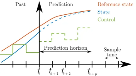
In MPC, an optimal control problem is solved on a short time horizon (theprediction horizon) while the real system (theplant) is running. Then the first entry of the optimal control is applied to the plant and the process is repeated with the time frame moving forward by onesample time h, see Figure9

Figure 9.Sketch of the MPC method. Due to the real-time constraints, the optimization problem has to be solved faster than the sample timeh.

In many MPC problems, stabilization of the system with respect to some reference state is the most important aspect. Nevertheless, there exist variations where stability is not an issue such that other (more economic) objectives can be pursued. These methods are known aseconomic MPC[126,127]. Another variation is the so-calledexplicit MPC[128], where the optimal control is computed in advance for a large number of different states and stored in a library. This way, the computational effort is shifted to an offline phase and during operation, we only have to select the optimal control from the library.

As in multiobjective optimal control, there are numerous applications where multiple objectives are interesting in feedback control. This means that we would have to solve the problem (MOCP) witht0 = ts andte = ts+prepeatedly within the sample timeh. It is immediately clear that even the simplest MOCPs cannot be solved fast enough to allow for real-time applicability. Consequently, efficient algorithms have to be developed which can be divided into approaches where one Pareto optimal solution is computed online and approaches with an offline phase during which the MOCP is solved2.

When implementing a MOMPC algorithm, one should keep in mind that – regardless of the algorithm used – the resulting trajectory need not be Pareto optimal, even if each single step is, cf. [129]. A remedy to this issue is presented in [130], where the selection of compromise solutions is restricted to a part of the Pareto front which is determined in the first MPC step. Due to this, upper bounds for the objective function values can be guaranteed.

4.1. Online multiobjective optimization

In the classical MPC framework, the optimal control problem is solved online within the sample timeh. Since it is in general impossible to approximate the entire Pareto set sufficiently accurately within this time frame, there are three alternatives:

1. compute a single Pareto optimal solution according to some predefined preference, 2. compute only a rough approximation of the Pareto set,

3. compute an arbitrary Pareto optimal control which satisfies additional constraints (e.g., stability).

In the first approach, the objective function is scalarized using, for instance, the weighted sum method (12) or the reference point method (13). In this situation, well-established approaches from scalar-valued MPC exist which one can build on. First results using the weighted sum method have appeared in [131]. In [132,133], the authors use the same scalarization for an MPC problem with convex objective functions. In this situation, it is guaranteed that any Pareto optimal solution can

2 _{In this article, algorithms where Artificial Neural Networks (ANN) have to be trained beforehand are nonetheless assigned}

be computed using weighted sums, and the weights can be adapted online according to a decision maker’s preference. Due to the convexity, stability can be proved for the resulting MPC algorithm. In [134], this approach is extended by providing gradient information of the objectives with respect to the weight vectorα. This way, the weights can be adapted in such a way that a desired change in

the objective space is realized. For non-convex problems, the weighted sum method is incapable of computing the entire Pareto set. Therefore, in [135], a variation of the reference point method is applied, where the targetTis the utopian point J∗, i.e. the vector of the individual minima. This way, also non-convex problems can be treated. In fact, due to the reference point method, the objective function is always convex [109] which can be exploited during the optimization. Alternative scalarization methods are thee-constraint method[136] orlexocographic ordering[137].

A disadvantage of a priori scalarization is that it is often difficult to select the scalarization parameter in such a way that a desired trade-off solution is obtained, and the remedy proposed in [134] is only applicable to a specific class of problems. Therefore, an alternative approach is to quickly compute a rough approximation of the entire Pareto set and then select the desired control online. Such methods have been proposed by many authors. The general approach is to us a MOEA and stop the computation after few iterations. In the next step, one of these suboptimal solutions is selected. This selection is realized by specifying a weight vector for the objectives in [138–141] and by the satisficing trade-off method in [142].

As a third option, we can compute a single Pareto optimal point without specifying which one we are specifically interested in as long as it satisfies additional constraints such as the stability of the system. Approaches of this type have been developed in [136] and [143], where a game theoretic approach is used.

4.2. Offline-Online decomposition

A well-known trick to avoid heavy online computations is to introduce an offline-online decomposition (very similar to meta modeling approaches where surrogate models are constructed before solving the MOCP). This means that the Pareto set is computed beforehand and in the online phase, an optimal compromise is selected according to a decision maker’s preference or some heuristic based on the system state or the environment.

Many of the approaches which fall in this category use a standard feedback controller instead of MPC, see [144] for a short review concerning methods using scalarization and offline PID controller optimization. In the offline phase, a Pareto set is computed for the controller parameters. Possible objectives are – among many others – overshooting behavior, energy efficiency or robustness. Algorithms of this type have been proposed in [145–147] using MOEAs and in [148–150] using set oriented methods.

An alternative approach is motivated by explicit MPC, i.e., the idea to solve many MOPs offline such that the correct solution can be extracted from a library in the online phase. Such a method has been proposed in [48]. In the offline phase, one has to identify all possible scenarios which can occur in the online phase. Such a scenario consists of both system states as well as constraints. This results in a large number of MOPs which have to be solved. In order to reduce this number, symmetries in the problem are exploited. To this end, a concept known asmotion primitives[151,152] is extended. In short, this means that if

arg min

u∈UMOP1=arg minu∈UMOP2,

where MOP1and MOP2are two problem instances from the offline library, then we only have to solve

0 1000 2000 3000 4000

p [m]

0 50 100

v

[k

m

/h

]

(i)

(i)

(i) (ii) (iii)

(iv) amin

amax

(a)

0 2000 4000 6000

p [m] 0

50 100

v

[

km h

]

ρ= 1

ρ= 0 ρ= 0.5

(b)

0 1000 2000 3000

50 100

v

[

km h

]

0 1000 2000 3000

p [m] 0

0.5 1

ρ

(c)

Figure 10.Results for the offline-online MPC approach from [48]. (a) Different constraint scenarios ((I)to(V I)), i.e., constant velocity, acceleration, deceleration, stopping. (b) Example track driven with the MPC algorithm. The red lines define the velocity bounds, the black dashed lines are trajectories corresponding to a constant weightα, and the green line is a trajectory where the weight is changed from 0 (energy efficient) over 0.5 (average) to 1 (fast). (c) Comparison between the MPC algorithm (coupled with a simple heuristic for the weighting) and the global optimum obtained via dynamic programming.

solutions which can be computed in explicit MPC for linear-quadratic problems, one has to rely on interpolation between solutions in the nonlinear setting.

4.2.1. Example: Autonomous driving

We here want to demonstrate the superiority of multiobjective approaches over scalar-valued MPC using the example of autonomously driving electric vehicles [47,48,153]. The problem there is to find the set of optimal engine torque profiles such that the velocity is maximized while the energy consumption is minimized. Additional constraints have to be taken into account such as speed limits or stop signs. The system dynamics are described by a four-dimensional, highly nonlinear ODE for the vehicle velocity, the battery state of charge and two battery voltage drops, cf. [153] for details. Numerical investigations reveal several symmetries in the system such that the only relevant state for a scenario is the current velocity whereas all other states only have a minor influence on the solution of the MOP. Consequently, the velocity as well as the constraints form the above-mentioned scenarios, see Figure10(a) for an illustration. For example, a scenario could be that the current velocity is 60 km/h and that the speed limit is currently increasing from 50 to 100 km/h, cf. scenario(I I)in Figure10(a). We then solve the MOP for this scenario and store the Pareto set in a library. By discretizing the velocity into steps of 0.1 (i.e.,v(t0) =. . . , 59.9, 60.0, 60.1, . . .), we have to solve 1727 MOPs in total in the offline

phase.

Table 2.Overview of publications (in chronological order) for multiobjective feedback control.

Algorithms without offline phase - computation of single points

Kerrigan et al. [131], Scalarization via weighted sum (WS) Wojsznis et al. [154]

Kerrigan & Maciejowski [155], Scalarization via lexicographic ordering He et al. [137]

Bemporad & Muñoz Scalarization via WS for convex objectives, guaranteed stability for de la Peña [132,133] large gain vs. noise robust stabilizing objectives

Geisler & Trächtler [134] WS, online adaptation of weights using gradient information

Maestre et al. [143] Scalarization via game-theoretic approach

Zavala & Flores- Scalarization via reference point approach Tlacuahuac [135]

Hackl et al. [129] Scalarization via WS for linear time-invariant (LTI) systems

Zavala [136] Scalarization viae-constraint: economic objective, stability as constraint

Grüne & Stieler [130] Economic objectives, performance bounds via selection criterion

Algorithms without offline phase - approximation of entire Pareto set

Laabidi et al. [138,140], Artificial neural network (ANN) for state prediction, optimization via Garcìa et al. [141] MOEA, selection of Pareto point via WS

Bouani et al. [139] ANN for state prediction, comparison of two MOEAs and WS for MOP

Nakayama et al. [142] Few MOEA iterations online, selection via satisficing trade-off method

Algorithms with offline phase

Fonseca [145], Offline computation of Pareto optimal controller parameters Herreros et al. [146] using MOEA

Scherer et al. [156] Robust control using a common Lyapunov function for multiple stability criteria

Ben Aicha et al. [147] Offline computation of Pareto optimal controllers parameters via EA and WS, online selection according to geometric mean of objectives

Krüger et al. [148] Offline computation of Pareto optimal controllers parameters via Set oriented methods, parametric model reduction for increased efficiency

Hernández et al. [149] Offline computation of Pareto optimal controllers parameters via Xiong et al. [150] simple cell mapping

Peitz et al. [48] Offline-online decomposition similar to explicit MPC

Applications

Zambrano & Camacho [157] MOMPC of a solar refrigeration plant via scalarization

Porfírio et al. [158] MOMPC of an industrial splitter using a min-max reformulation

Pedersen & Yang [159] MO PID controller design for magnetic levitation systems via MOEA

Li et al. [160] Multiobjective adaptive cruise control for vehicles

Hu et al. [161] MOMPC of high-power converters via WS

Núñez et al. [162] MOMPC of dynamic pickup and delivery problems using MOEA

green line corresponds to a varying weight. This way, a flexible cruise control is established where the driver can quickly adapt, for instance, to changing energy requirements.

As has been mentioned before, an alternative to interactively choosing a weight is to implement some heuristic which automatically chooses a weight based on the current situation. Such an approach is visualized in Figure10(c), where the weighting depends on the vehicle velocity as well as on current and future velocity constraints. For a simpler track it is possible to compute a globally optimal solution for a scalarized objective using dynamic programming. We see that with the heuristic, the MOMPC approach yields trajectories close to the global optimum while only having finite horizon information.

4.3. Summary

We again conclude the section by giving a summary of publications where multiobjective optimization is applied in a real-time context. The publications are divided into four categories. The first two contain algorithms where the MOP is solved online. The categories differ in whether a single point is computed or the entire set is approximated. Consequently an offline phase is not required except in the case where surrogate models are trained in order to accelerate the online computations. The third category then contains the methods with an offline optimization phase, and some applications are mentioned in the fourth category.

5. Reduction techniques for many-objective optimization problems

Another important restricting factor in multiobjective optimization is the number of objectives [164]. For MOPs with four or more objectives, the termmany-objective optimization (MaOP)has been coined and over the past years, many researchers have dedicated their work to address MaOPs and the issues arising from thecurse of dimensionality, cf. [165] for an overview, [166,167] for new concepts for identifying non-dominated solutions and [168–172] for evolutionary approaches.

A popular approach for MaOPs are interactive methods [173–178]. These methods do not compute the entire set of optimal compromises but instead interactively explore the Pareto set. Starting at the current Pareto optimal solution, adecision makercan choose in which direction to proceed, i.e., which objective to improve at the expense of some other, currently less important objective. The approach in [178], for example, allows for Pareto optimal movements both in decision and objective space. One of the main advantages of interactive methods, is the reduced computational effort – especially in the presence of many criteria – since it is not affected significantly by the dimension of the Pareto set. Moreover, this way decision making from a vast number of Pareto optimal solutions is avoided which can be overwhelming for a decision maker. Consequently, interpretability and usability are increased.

Besides interactive methods, several reduction techniques have been proposed in the context of many-objective optimization and although it is not the main theme of this review article, we want to give a brief overview of these reduction approaches since they also aim at increasing the efficiency of solving MOPs. These reduction techniques can be divided into two main categories. The first one isobjective reduction, where the aim is to reduce the number of objectives while (approximately) preserving the Pareto set. The observation behind this is that not all objectives are of equal importance to the structure of the Pareto set, which is measured by thedegree of conflict[179]. Consequently, when it is possible to identify the main contributors to the Pareto set, then one can solve a reduced problem taking into account only these most important objectives. Different approaches have been proposed for this identification step, all of which use a set of sample points. In [179], both exact and inexact algorithms are proposed for selecting a subset of objectives such that only those points in the Pareto set are lost which are worse in all remaining objectives by a constantδor more. This approach is also

(a) (b) (c)

Figure 11.Visualization of the hierarchical structure of Pareto sets. (a) Pareto set of an example problem withJ:R3→R4. (b) The four Pareto sets taking only three objectives into account form the boundary

of the original Pareto set. (c) The Pareto sets in (b) are again bounded by the respective bi-objective subproblems.

The method proposed in [187] possesses characteristics of the first category – namely objective reduction – as well as of the second category which is the exploitation of the structure of Pareto sets and front. Therein, first thecornersof the Pareto front are identified and this information is used to select the relevant objectives. Algorithms of the second type all exploit this hierarchical structure. This means that in under certain assumptions, the Pareto front is bounded by the Pareto fronts of subproblems where one or more objectives have been neglected, cf. [188,189]. This way, the solution can be computed by a hierarchical approach where – starting with scalar problems – the boundary is computed before finally the interior is obtained. Very recently, results about the hierarchical structure of the Pareto set, i.e., in decision space, have appeared, see [73,190] for details. This approach is illustrated in Figure11where the solution to an MOP with four objectives is shown as well as the Pareto sets of the subproblems with three and two objectives, respectively.

6. Future directions

This survey has given an overview over recent advances in the context of accelerating multiobjective optimization. These are surrogate models, feedback control and objective reduction techniques. Similar to almost every other field of science, it can be expected that the immense developments in data-based methods will also have a major impact on research in multiobjective optimization, in particular in the context of surrogate modeling. A very large number of researchers from the dynamical systems community is working on data-based methods using theKoopman operator, which is an infinite-dimensional but linear operator describing the dynamics of observables [191,192]. Significant effort has been put into the development of numerical methods for approximating this operator from data, see, e.g., [193,194]. This way, the dynamics of observations can be reconstructed entirely from data and without any knowledge of the underlying system dynamics. In a way, this allows is to merge the two surrogate modeling categories from Sections3.2and3.3since we can approximate the dynamics not only of the state but directly of the objectives. Several methods have recently been proposed to use the Koopman operator for data-based controller design, both in simulations [195–198] as well as experiments [199,200]. The results are very promising such that it is just a matter of time until these methods are utilized for multiobjective optimal control.

In the same manner, machine learning techniques [201] will very likely gain more and more attention, both in multiobjective optimization as well as optimal control. There are already many papers on this topic or related ones and the number is growing quickly.

Reference

1. Knowles, J.; Nakayama, H. Meta-Modeling in Multiobjective Optimization. InMultiobjective Optimization: Interactive and Evolutionary Approaches; Branke, J.; Deb, K.; Miettinen, K.; Slowinski, R., Eds.; Springer Berlin Heidelberg, 2008; pp. 245–284.

2. Tabatabaei, M.; Hakanen, J.; Hartikainen, M.; Miettinen, K.; Sindhya, K. A survey on handling computationally expensive multiobjective optimization problems using surrogates: non-nature inspired methods. Structural and Multidisciplinary Optimization2015,52, 1–25.

3. Chugh, T.; Sindhya, K.; Hakanen, J.; Miettinen, K. A survey on handling computationally expensive multiobjective optimization problems with evolutionary algorithms.Soft Computing2017, pp. 1–30. 4. Miettinen, K.Nonlinear Multiobjective Optimization; Springer Science & Business Media, 2012. 5. Ehrgott, M.Multicriteria optimization, 2 ed.; Springer Berlin Heidelberg New York, 2005.

6. Hindi, H.A.; Hassibi, B.; Boyd, S.B. MultiobjectiveH₂/H_∞-Optimal Control via Finite Dimensional Q-Parametrization and Linear Matrix Inequalities. Proceedings of the American Control Conference, 1998, pp. 3244–3249.

7. Zhu, Q.J. Hamiltonian Necessary Conditions for a Multiobjective Optimal Control Problem with Endpoint Constraints. SIAM Journal on Control and Optimization2000,39, 97–112.

8. Gambier, A.; Badreddin, E. Multi-objective optimal control: An overview. 16th IEEE International Conference on Control Applciations, 2007, pp. 170–175.

9. Tröltzsch, F. Optimal Control Of Partial Differential Equations. Graduate studies in mathematics2010,112. 10. Hinze, M.; Pinnau, R.; Ulbrich, M.; Ulbrich, S.Optimization with PDE Constraints; Springer Science+Business

Media, 2009.

11. Ober-Blöbaum, S. Discrete Mechanics and Optimal Control. PhD thesis, University of Paderborn, 2008. 12. Schilders, W.H.A.; van der Vorst, H.A.; Rommes, J. Model Order Reduction; Springer Berlin Heidelberg,

2008.

13. Karush, W. Minima of Functions of Several Variables with Inequalities as Side Constraints. Master thesis, University of Chicago, Illinois, 1939.

14. Kuhn, H.W.; Tucker, A.W. Nonlinear programming. Proceedings of the 2nd Berkeley Symposium on Mathematical and Statsitical Probability. University of California Press, 1951, pp. 481–492.

15. Romaus, C.; Böcker, J.; Witting, K.; Seifried, A.; Znamenshchykov, O. Optimal energy management for a hybrid energy storage system combining batteries and double layer capacitors. Energy Conversion Congress and Exposition, 2009. ECCE 2009. IEEE. IEEE Xplore Digital Library, Los Alamitos, 2009, pp. 1640–1647.

16. Hillermeier, C.Nonlinear Multiobjective Optimization: A Generalized Homotopy Approach; Birkhäuser, 2001. 17. Schütze, O.; Dell’Aere, A.; Dellnitz, M. On Continuation Methods for the Numerical Treatment of

Multi-Objective Optimization Problems. Dagstuhl Seminar Proceedings, 2005.

18. Deb, K.Multi-objective optimization using evolutionary algorithms; Vol. 16, John Wiley & Sons, 2001. 19. Coello Coello, C.A.; Lamont, G.B.; Van Veldhuizen, D.A.Evolutionary Algorithms for Solving Multi-Objective

Problems; Vol. 2, Springer Science & Business Media, 2007.

20. Zitzler, E.; Laumanns, M.; Thiele, L. SPEA2: Improving the Strength Pareto Evolutionary Algorithm. TIK-Report 1032001.

21. Deb, K.; Pratap, A.; Agarwal, S.; Meyarivan, T. A Fast and Elitist Multiobjective Genetic Algorithm: NSGA-II.IEEE Transactions on Evolutionary Computation2002,6, 182–197.

22. Zhou, A.; Qu, B.Y.; Li, H.; Zhao, S.Z.; Suganthan, P.N.; Zhang, Q. Multiobjective evolutionary algorithms: A survey of the state of the art.Swarm and Evolutionary Computation2011,1, 32–49.

23. Ong, Y.S.; Lim, M.H.; Chen, X. Memetic Computation—Past, Present & Future. IEEE Computational Intelligence Magazine2010,5, 24–31.

24. Neri, F.; Cotta, C.; Moscato, P.Handbook of memetic algorithms; Vol. 379, Springer, 2012.

25. Schütze, O.; Alvarado, S.; Segura, C.; Landa, R. Gradient subspace approximation: a direct search method for memetic computing. Soft Computing2016.