3D Full-Wave modelling and EC mode conversion in realistic plasmas
PavelAleynikov1,∗and Nikolai B.Marushchenko1
1Max-Planck-Institut für Plasmaphysik, Greifswald, Germany
Abstract.The wave physics of O-X conversion in overdense W7-X plasma is discussed. For this study, a new 3D, cold plasma full-wave code has been developed. The code takes advantage of massive parallel computations with Graphics Processing Units (GPU), which allows for up to 100 times faster calculations than on a single-CPU. A 3D calculation of the O-X conversion is demonstrated. We discuss limitations of the mode conversion scenario within the capabilities of the existing ECRH system in W7-X, and demonstrate an optimised conversion scenario in which the launching antenna location is altered. The conversion efficiency of the optimised scenario is predicted to be>85%.
1 Introduction
Electron Cyclotron Resonance Heating (ECRH) is the main plasma heating mechanism in Wendelstein 7-X (W7-X) Stellarator. It is provided by 10 gyrotrons at 140 GHz (corresponding to the second harmonic cyclotron reso-nance at 2.5 T) with the power of 1 MW each. X- and the O-modes were successfully used in a wide range of operation scenarios: X-mode for low and moderate den-sities (up to the cutoff at 1.2·1020m−3), and O2-mode
for higher densities (up to 2·1020m−3). Possible
opera-tion at yet higher densities would involve double mode-conversion from O- to slow X- and to Bernstein-mode, i.e. an OXB-scenario. The physics of O-X conversion is out-side of applicability of the routinely used geometrical op-tics approximation (WKB-theory) and should be consid-ered within a full-wave approach.
This work reports on the development of a new 3D cold plasma full-wave code, named CUWA. The code uti-lizes the Finite Difference Time Domain (FDTD) tech-nique [1, 2] and has an interface with the ray-tracing code TRAVIS [3]. The computation domain is “minimized” around the WKB-trajectory obtained from the ray-tracing code by means of the Convolutional Perfectly Matched Layer (CPML) technique [4]; the background magnetic field is recovered from pre-computed 3D equilibrium data. The code takes advantage of massive parallel computa-tions with Graphics Processing Units (GPUs), which al-lows for up to×100 acceleration over a single-CPU.
2 Numerical model
FDTD (also known as Yee’s method) is a standard tech-nique for full-wave simulations in various branches of physics [1, 2]. In fusion plasmas, it has been successfully applied to study wave propagation, O-X conversion [5], re-flectometry [6] and the scattering of EC waves on plasma
∗e-mail: [email protected]
turbulence [7]. In this work we mostly follow the FDTD method as given in Chapter 11.3 of [2], with two impor-tant differences: first, we modify the current discretisation scheme and, second, we amend the differential operators of Maxwells equations in the boundary layers in accor-dance with the CPML technique [4] (see below).
The system of equations been solved is Maxwell’s equations with addition of a “cold plasma” response cur-rent equation (J) given by the electron law of motion:
∂
∂tB=−∇ ×E,
∂ ∂tE=c
2∇ ×B−J/ε
0,
d
dtJ+νJ=ε0ω
2
pE−J×ωc,
(1)
whereω2p =nee2/ε0meis the plasma frequency,νis
elec-tron collisional frequency and ωc = |e|B0/me is the
cy-clotron frequency corresponding to the background mag-netic field,B0.
In the FDTD method the field components are discre-tised on staggered grids in space and time. Note that is it common to discretize the plasma-response curren,J, in such a way that itsJx,JyandJzcomponents are co-located
in space [2, 5]. This facilitates the current update calcu-lation. However, we find the stability of this scheme to be unsatisfactory, in particular when applied to the CMPL region. Therefore we have implemented a slightly more computationally demanding but more stable scheme where
Jis discretized in the same way as the wave electric field,
E. This implies that the the current update equation will involve interpolation of its components.
3 Perfectly matched layer
domain [5, 7]. In such a case one would need to amend the computation domain with layers of “many-wavelengths” thickness at each boundary ensuring smallness of reflected signals. This may become problematic in 3D calculations when the domain of interest itself has the size of a few wavelengths. Amending such a domain with six boundary layers may significantly reduce the overall efficiency.
A so-called CPML boundary [4] is instead imple-mented in our full-wave code to truncate the computation domain. An efficient CPML requires only a few extra Yee cells in each direction - i.e. a fraction of a single “wave-length”. CPML also requires two auxiliary (virtual) 3D fields (ψ) for each component ofEandB, i.e. 12 auxiliary fields in total. However, these auxiliary fields are defined only within the narrow CPML layers, resulting in a negli-gible overhead in the practical setup.
The conceptual idea behind CPML [4] can be sum-marised in the following way (further details and a rather complete overview of various PMLs can be found in the book [8]). CPML is an efficient numerical implementa-tion of Complex Frequency Shifted PML [9], in which the differential operators in Eqs. (1) are replaced with the con-volution:
∂ ∂u → L
−1
(
1 κu+αu+σiuωε0
) ∗ ∂
∂u,(u=x, y,z), (2)
whereL−1{F(ω)}denotes inverse Laplace transform and
(κu, αu, σu) are free parameters accounting for
coordi-nate stretching in real and complex plains and an “effective conductivity”. PML given by Eq. (2) introduces no reflec-tions because it can be viewed as a vacuum with complex-stretched coordinates. In other words, with Eq. (2) the so-lution of Eq. (1) isanalyticallycontinued into the complex plain with a subsequent mapping of the complex coordi-nates back to real space but with a “complex material”.
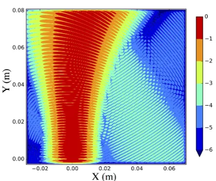
In order to demonstrate CPML performance for the FDTD realisation described above we design a benchmark which represents a general anisotropic scenario. In this scenario, a divergent Gaussian beam propagating through the plasma escapes from the computation domain through a strongly nonuniform boundary. The entire computation domain is surrounded by the narrow CPML layer. This is shown in Fig. 1, the wave is launched vertically from the origin (0,0). The plasma density ranges from 0 to ap-proximately 80% of the O-mode cut-off with a gradient directed diagonally (bottom right to top left). It can be seen that at the top PML layer the wave-front incident an-gle varies from almost normal to quite oblique, ensuring extended benchmarking. The resulting reflection error is estimated as a maximum value of the electric field ampli-tude recorded in the bottom-right quarter of the domain. Note that the maximum relative error reported in the orig-inal work [4] is≈5·10−4. Similar reflection is observed
in our benchmark case (a wave with the cyan contours [10−4; 10−3]). Note the presence of another wave going
out through the top right corner (contours [10−5; 10−4]).
This spurious wave is associated with an inaccuracy of the Gaussian beam setup at the bottom boundary. Frequently, CPML outperforms the initial condition accuracy (for in-stance in a typical case where PML lies in vacuum) then
Figure 1. A snapshot of the decimal logarithm of the waveE
-field magnitude for a CPML benchmark case.
the latter becomes the dominant noise source (i.e. intro-duces∼10−4error in field amplitude). Note that the rela-tive errors are squared when the intensity or mode power is of interest. The above example is calculated with the resolution of 12 Yee cells per vacuum wavelength and a CPML size of 12 cells.
4 Mode conversion examples
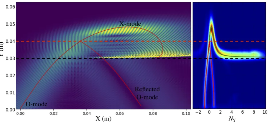
One of the applications of our code is the calculation of the O- to X-mode conversion efficiency in 3D plasmas.
Figure 2.An example of an O-X mode conversion calculation. Left plot: snapshot of the wave electric field (color-coded), ray tracing (solid red). The antenna is located in the bottom left corner. The O-mode cutoffand Upper Hybrid resonance layers are indicated with red and the black dashed lines, respectively. Right plot: windowed Fourier transform of the wave field, i.e wave refractive index (color-coded) and the refractive index predicted by ray-tracing (solid).
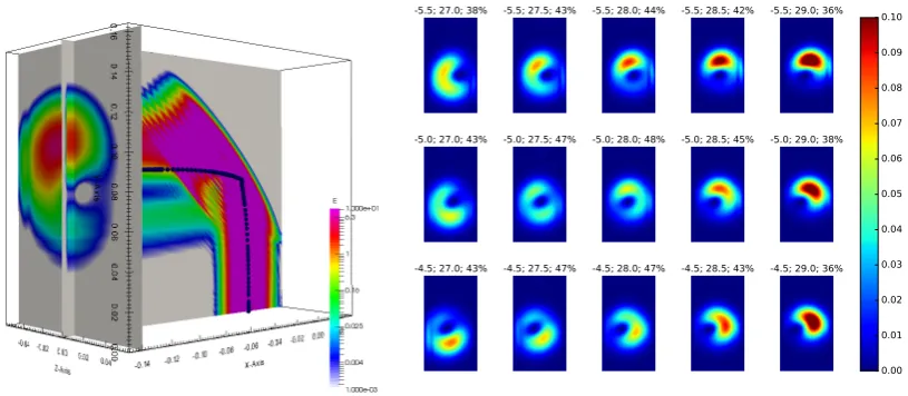
contained within the computation domain, the reflected O-mode power distribution is shown on the planex=const). The decimal logarithm of the time-averagedE2 is colour-coded. The sequence of dark-colored points represents the corresponding WKB trajectory for the reference ray. It is evident from the peculiar cross-section of the reflected wave that the 3D geometry needs to be appropriately ac-counted for.
To estimate the power conversion efficiency, we com-pute surface integrals of the time-averaged Poynting vector (i.e. the intensity) over every boundary of the computation domain. In the above case, the OX conversion efficiency can be calculated as the difference between the intensities of the input (Sin) and reflected (Sref) waves. An
estima-tion of the OX conversion efficiency is made as follows for W7-X-relevant ECRH beam parameters and plasma geometry. A Gaussian beam approximation is used as an initial condition. A beam of 2 cm radius and a phase front curvature of 1 m approximates the ECRH beam at the plasma entrance. The density profile is chosen arbi-trarily (with a normalized gradient of ≈ 20m−1 near the
cutoff). The antenna launcher location was fixed, corre-sponding to the upper port “A, C1” in W7-X nomencla-ture. Then, the launcher azimuth and altitude angles were varied to find direction for highest OX conversion. We find that for the given conditions (equilibrium, density profile, launcher position and beam focusing) the maximum con-version (Sin −Sref)/Sin reaches 48% (the middle tile in
Fig. 3 (right)).
5 Optimised conversion scenario in W7-X
It appears that∼50% is a typical maximimum conversion fraction for realistic W7-X beam parameters (focusing and
width were optimized) and launcher positions. Refs. [10– 12] suggest that conversion can be improved by a careful design of the beam wavefront. In this report we pursue an alternative optimisation strategy.
We take advantage of the fact that stellarator equilib-rium “offers” a wide variety of magnetic field curvatures on a cutoffsurface (flux surface), and we search for a loca-tion which would minimise the thickness of the evanescent layer, weighted over the beam radial profile. The thickness of the evanescent layer at the O-mode cutoffsurface is esti-mated using the results of analytical theory [13], where the thickness is taken to be the distance (in wave-vector space) between the WKB solutions of the two modes. This esti-mate is known to agree very well with calculations in a flat 2D case [5].
The result of this calculation is demonstrated in Fig. 4 (left). The function representing the Gaussian-weighted gradient of the thickness of the evanescent layer is plot-ted on the cutoff surface, which is parametrized by the poloidal and the toroidal angles. A few minima of this function are marked with red dots. A different opti-mal value of parallel refractive indexN||opt corresponds to each minimum due to the variation of the magnetic field strength on the surface.
It is easy to understand the “meaning” of these spe-cial points. We recall that the efficient conversion occurs when the “turning” points for the wave-packets of the two modes (O- and slow X-) are close to each other. For-mally, the conversion condition is satisfied at the intersec-tion of two surfaces: the O-mode cutoffsurface and the X-mode turning surface parameterised by the plasma fre-quency (ωp), the cyclotron frequency (ωc), and the wave
in--5.5; 27.0; 38% -5.5; 27.5; 43% -5.5; 28.0; 44% -5.5; 28.5; 42% -5.5; 29.0; 36%
-5.0; 27.0; 43% -5.0; 27.5; 47% -5.0; 28.0; 48% -5.0; 28.5; 45% -5.0; 29.0; 38%
-4.5; 27.0; 43% -4.5; 27.5; 47% -4.5; 28.0; 47% -4.5; 28.5; 43% -4.5; 29.0; 36%
0.00 0.01 0.02 0.03 0.04 0.05 0.06 0.07 0.08 0.09 0.10
Figure 3.3D calculation of the scenario similar to the one described in Fig. 2 (left). Reflected O-mode shape for various aiming angles
of the launched beam (right).
0 5 10 15 20 25 30 35
ϕ 0
100 200 300
θ
Figure 4.Left: Location of the optimal conversion regions (red dots) on the cutoffsurface (φandθare toroidal and poloidal angles).
The function representing the weighted gradient of the thickness of the evanescent layer is colorcoded. Middle: Conversion region for N||opt≈0.564. Right: Optimised efficient conversion region forNopt|| ≈0.5632 (φ≈3.5 andθ≈190 on the left plot).
tersection curve (3D-shaped, in general) will vary withN||. Fig. 4 (middle) shows this intersection forN||opt ≈0.564, where the surfaces cross each other obliquely and thus the evanescent layer is narrow only close to the intersection (if the beam has a constantN||structure). WhenN|| corre-sponds to one of the optimised locations, the intersection has a more complex structure (a saddle point in an example of Fig. 4 (right)), ensuring minimisation of the evanescent layer weighted over a finite Gaussian beam.
The location of the conversion region in plasmas (and thusNopt|| ) uniquely defines the O-mode ray which arrives to this point within the WKB approximation. Therefore the beam launching location and angles can be computed with a backward ray-tracing calculation (staring from the conversion region). When the initial conditions for the beam outside of plasma are known, the full-wave calcu-lations are done to predict the conversion efficiency. The maximised conversion efficiency predicted with our full-wave code for a case of Fig. 4 (right) reaches a remarkable 85%.
Note that such an algorithm for an identification of an optimised conversion scenario implies that the wave launcher location can be chosen freely. This is generally not the case in W7-X. Therefore our future plans include a study in which various W7-X equilibria are analysed in or-der to identify those where the optimal conversion regions are accessible within the capabilities of the existing ECRH system.
References
[1] A. Taflove, S.C. Hagness,Computational Electrody-namics: The Finite-Difference Time-Domain Method (ARTECH HOUSE INC, 2005), ISBN 1580538320, [2] U.S. Inan, R. A.Marshall, Numerical Electromag-netics: The FDTD Method (Cambridge University Press; 1 edition, 2011), ISBN 052119069X,
[3] N. Marushchenko, Y. Turkin, H. Maassberg, Com-puter Physics Communications185, 165 (2014) [4] J.A. Roden, S.D. Gedney, Microwave and optical
[5] A. Köhn, Á. Cappa, E. Holzhauer, F. Castejón, Á. Fernández, U. Stroth, Plasma Physics and Con-trolled Fusion50, 085018 (2008)
[6] J.H. Irby, S. Horne, I.H. Hutchinson, P.C. Stek, Plasma Physics and Controlled Fusion 35, 601 (1993)
[7] T.R.N. Williams, A. Köhn, M.R.O. Brien, R.G.L. Vann, Plasma Physics and Controlled Fusion 56, 075010 (2014)
[8] J.P. Berenger, Perfectly Matched Layer (PML) for Computational Electromagnetics(Morgan and
Clay-pool Publishers, 2007), ISBN 1598290827,
[9] M. Kuzuoglu, R. Mittra, IEEE Microwave and Guided wave letters6, 447 (1996)
[10] A.G. Shalashov, E.D. Gospodchikov, Plasma Physics and Controlled Fusion52, 115001 (2010)
[11] E.D. Gospodchikov, T.A. Khusainov, A.G. Sha-lashov, Plasma Physics and Controlled Fusion 54, 045009 (2012)