Deep Learning vs Templates Attacks in front of
fundamental targets: experimental study
Yevhenii Zotkin, Francis Olivier, Eric Bourbao
GEMALTO Hardware Security Labs, La Ciotat, France
francis.olivier,[email protected]
December 20, 2018
Abstract
This study compares the experimental results of Template Attacks (TA) and Deep Learning (DL) techniques called Multi Layer Perceptron (MLP) and Convolutional Neural Network (CNN), concurrently in front of classical use cases often encountered in the side-channel analysis of cryptographic devices (restricted to SK). The starting point regards their comparative effectiveness against masked encryption which appears as intrinsically vulnerable. Surprisingly TA improved with Principal Com-ponents Analysis (PCA) and normalization, honorably makes the grade versus the latest DL methods which demand more calculation power. An-other result is that both approaches face high difficulties against static targets such as secret data transfers or key schedule. The explanation of these observations resides in cross-matching. Beyond masking, the effects of other protections like jittering, shuffling and coding size are also tested. At the end of the day the benefit of DL techniques, stands in the better resistance of CNN to misalignment.
1
Introduction
1.1
The advent of Deep Learning in supervised methods
Supervised attacks consider 2 phases called learning phase (a.k.a profiling) and a test phase (a.k.a matching). In the learning phase the cryptographic Device Under Test (DUT) is assumed open. So the secrecy chunks can be set freely with every values and the traces associated accordingly in order to build up a -hopefully bijective- model that maps the value onto the signal. The test phase applies this model on the locked twin DUT to be attacked: its aims at identifying the chunks of secret values by submitting to the model the signal produced while playing a comparable process as in learning phase. The portability issues regards the difficulty of reproducing the same measurement conditions in both phases so as to preserve the signals compatibility and keep them comparable.
Template attacks (TA) are well knwon for 20 years now and based upon sound classical statistics [13, 7]. They are based upon Bayesian inference and multivariate Gaussian behavior (see formulation inappendix A). Some improve-ments have been proposed in 2006 by Archambeau et al. [2] with Principle Components Analysis (PCA) originally introduced to facilitate the identifica-tion and management of thepoints of interest (POI) within the signals. TA are seen as theoretically optimal [35] but perceived as poorly effective on the field: they are difficult to implement in practice; their requirements are seldom encountered because open DUTs are not often available for learning and the portability remains as a hard point (when profiling and matching are not con-ducted on the same DUT). Besides they are considered as easily thwarted with some well-known countermeasures that will be discussed in this paper.
New techniques derived from Artificial Intelligence, Machine Learning, Neu-ral Networks have recently been introduced into the scope of supervised SCA [23, 24]. With the help of important computational resources (memory and cal-culation power), they prove to be applicable, generic and effective. Following Benadjila et al. [4] two of them are implemented in this study and designated by MLP (MultiLayer Perceptron) and CNN (Convolutional Neural Network). These methods are interesting and challenging for classical TA methods because have been presented as capable of circumventing some known protections that defeat TA such as random boolean masking and jittering.
An important remaining issue regards the portability referring to the fact that the learning and test phases might have not been conducted against the same device and/or under the same measurement conditions. Moreover a basic issue in test/matching phase remains the amount of the candidate traces. We will see in this study that, as the DL techniques, TA can also apply some preprocessing to the traces such as normalization and PCA.
1.2
Typology of targets
new targets: secret transfers (key loading), key scheduling or poorly exposed encrypted data (secret codes or cryptograms). We designate thesef(K) cases asstatic targetsbecause the secret data do not change during the test phase. Conversely encryption f(K, M) can be designated as a potentially dynamic target because the message varies in test phase. For sake of simplicity we follow many papers and target the firstSubByte function at the beginning of the AES algorithmSBox(Ki⊕Mi) to illustrate this kind of target although the DES first round could be considered as well. These are typically the targets of non-profiled attacks DPA/CPA [21, 5, 20] but they are often addressed by the supervised ones for the following reasons:
• Regardless of their applicability, supervised attacks may succeed with less traces during the test phase than the amount required for statistical esti-mation as in CPA for instance.
• The message variability can be considered as a workaround to relieve the open device requirement of the learning phase. As long as only the leakages ofKi⊕Mi(input) and SBox(Ki⊕Mi) (output) are observed, no need to vary the key anymore, only to know it! Key loading and scheduling are excluded.
1.3
Cross matching
Let’s take this opportunity to introduce the notion of cross-matchingwhich is specific todynamic targets. Of course if the classes are labelled at profiling according to the exclusive-OR valueK⊕M, the matching will have to redirect the comparisons labels throughK∗=M∗⊕K⊕M , ifK∗ (the unknown) and
M∗ (supposedly known) designate the variables in test phase.
1.4
Classical protections
1.4.1 Jittering
Traces jittering designates a random misalignment implemented by any kind of hardware and software means (clock instability, fake cycles, additional random code insertion). It must be implemented as a minimal countermeasure. But if too simplistic its effect can sometimes be cancelled by the attacker with signal preprocessing and pattern matching. If not fixed it is effective against many kinds of SCA. But some most recent techniques show to be insensitive to it and designed in that purpose.
1.4.2 Shuffling
but unfortunately less used in data transfers routines. Here again some new analysis techniques aim at mitigating it.
1.4.3 Masking
Boolean masking [11] replaces natural encryption functions by randomized vari-ables such asSBox0(Ki⊕Mi⊕u) =SBox(Ki⊕Mi)⊕v with modifiedlook-up
tables(LUT) and random masksuandvinternally refreshed at each execution. The objective is to make variables unpredictable (It is also used in key schedul-ing but rather poorly in data transfers). It is well known in the domain of non-profiles attacks that this sort of implementation is prone to second order analyses [27, 14, 12] the secret key can be inferred if the random mask and the masked variable leakages are observed jointly soas to exploit their mutual dependence. But so far data masking undermined TA methods except is very unrealistic conditions (simplistic and noise free leakages, known mask at profil-ing!). As a matter of fact masking requires 2ndorder DPA for POI identification (SNR, SOST become powerless). The variable leakage turns multifaceted for each value and the templates all equivalent!
1.4.4 Coding size
Coding size refers to the size of the machine words or registers that host the internal variables (from 8, 16, 32, 64, 128 bits to more exotic values in hardware coprocessors). Splitting the data into words as imposed or proposed by the hardware architecture has a major impact on the applicability of supervised attacks. This topic is insufficiently discussed in papers that mainly deal with 8 bits implementations. It will be addressed along with the static targets. In 2014 an interesting and daring study has been proposed by Choudary and Kuhn [9] aiming at a full extension to 16 bits, with partitioning over 65536 classes! Unfortunately they deal with a couple of successive bytes that leak successively and not simultaneously. Beyond the digital acquisitions and data management difficulties, working with numerous classes raises estimation problems. So this paper will just consider the realistic case of 8 bits partitioning (which could be extended to 10 or 12) whereas the leakage is due to 16 bits (or 32) at the same time.
1.5
Experimental purpose of this paper
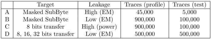
Target Leakage Traces (profile) Traces (test) A Masked SubByte High (EM) 45,000 5,000 B Masked SubByte Low (EM) 900,000 100,000 C 8 bits transfer High (power) 900,000 100,000 D 8, 16, 32 bits transfer Low (EM) 500,000 500,000
Table 1: Designation of the datasets.
Concurrent analyses of TA and DL (MLP and CNN) will be experienced against 4 targets all operated in favorable experimental conditions, free of any portability issue: the acquisitions set-up are the same and consistent for both learning and test phases.
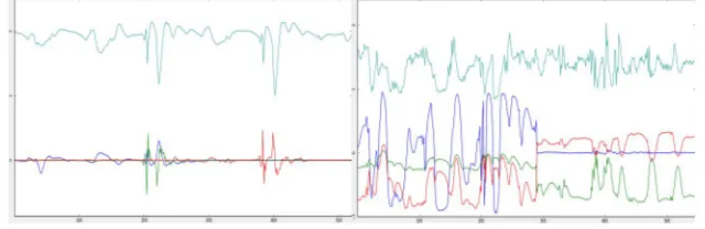
Target A refers to the public ASCAD dataset (MNIST dataset from [4]). It consists of 50,000 training and 10,000 testing traces of 700 electromagnetic (EM) samples from an ATMega8515 microcontroller performing the first round of AES encryption. Target variable is an output of the second byte masked AES SBox. Therefore dataset poses 256-class classification problem. For testing purpose the mask is also known with the message and can be used or not. There exist 3 versions of dataset: one without jittering and 2 with jittering simulated by randomly shifting. Jittering effects will be testes on this special implementation. Target B refers to another hardware implementing also masked AES substi-tution. Two sets of data are available with or without shuffling (but no jittering) and monitored through both EM and power signals. The leakage is much weaker but 1 million traces are available in each set.
Target C is a simplistic 8 bit data transfer implemented on a old chip for smart card and strongly leaking the data through its power reaching CPA rates up to 0.6.
Target D is a realistic chip for smart card monitored with EM and imple-menting data transfers with various word sizes: 8, 16, 32 bits, with or without shuffling. CPA leakage rates stand between 0.1 to 0.15.
This paper starts with a bibliographic overview of the supervised methods applied to the SCA problems. Then DL-MLP and DL-CNN techniques are experienced on dynamic targets A and B. The following section does the same with TA improved by PCA and normalization. Thenstatic targetsare tested with both DL and TA methods before a final synthesis of the results draws some basic practical lessons out of these experiments.
2
Literature overview
2.1
Template attacks
Template attacks are the profiling attacks holding the assumption that attacker is in possession of an identical copy of the cryptographic device being attacked (DUT). TA consists in collecting a large time signal made of N samples for each operationOi(which in machine learning terminology would correspond to classification problem with|O|=K classes). By the way the classical gaussian formulation of TA (textitappendix A) is named Quadratic Discriminant Analysis (QDA) in regular statistics (and used in machine learning terminology).
Typically, classical papers consider operations processed by a 8-bit micro-controller for which there areK = 256 possible values. Surprisingly the issue related to the size of the selection variable has been very lately addressed in literature for data transfers [9] and key schedule [36]. The other types of pro-tections are considered as rather weak but relatively effective when combined jointly. Let’s notice that from 2007 Oswald et al. [29] have addressed the issue of TA against boolean masking but under so unrealistic assumptions (profil-ing with known mask!) that mask(profil-ing is generally also recommended as a good protection.
2.2
Principal component analysis
A major problem of the template attacks is the dimensionalityN of the input samples. Typically N is O(105) depending on the sampling rate of an oscil-loscope. A lot of research effort has been invested to find the optimal way to project data in low dimensional subspaces while maximizing the predictive power of the features. To address this issue Archambeau et al. [2] proposed to perform attacks in principal subspaces, using PCA [18] projection both as the dimensionality reduction tool and as an automated way to more efficiently select the points of interest POI (see appendix B). They performed successful attacks against secret key ciphers. In the case of AES, the attack was conducted on a non-masked implementation of the algorithm. To our best knowledge, there is no published literature on the use of the template attacks with PCA on masked implementations.
Prior to likelihood computation, PCA projects the vectors and matrices (see
appendix B) into a linear sub-space. The projection matrix results from an Eigen problem applied to the inter-classes scatter matrix S =E[(Tk−T)(Tk−T)T] which is the related to the global and classes covariance matrices byR=E[Rk]+
S (literally the ”variance of the average templates” plus the ”average of the covariances” taken over all classesk). Furthermore it may also apply toR−1Sas a kind of SNR criterion maximizing inter-classes scattering over global scattering and noise (a.k.a Linear Discriminant Analysis LDA [33]). The choice of matrix
2.3
Machine Learning based methods
The first attempt of using Machine Learning methods dates from 2002 [31], where authors were using Kohonen Neural Networks to learn from electromag-netic signatures. Later in 2012, people were using Support Vector Machine (SVM) instead of TA to get rid of the issue of the underlying Gaussian hypoth-esis of the latter [1]. Other non-parametric approaches have also been shown to be competitive with TA [16, 24]; drawbacks have been highlighted though, such as increased computational power or other non-decidable issue as the choice of the hyper parameters. More recently, neural network approaches showed up to attack an AES implementation [26].
2.4
Deep learning based methods
To our best knowledge, the first publication on using Deep Learning models for side-channel attacks is by E. Cagli et al. in 2017 [6]. The authors use Convolutional Neural Networks [22] to perform an attack on a non-masked im-plementation of AES. In their perspective, primal interest in using CNN comes from the problem of traces alignment. Raw traces always come with some form of random misalignment from one trace to the other due to natural jittering, hardware countermeasures or software desynchronization. Post-alignment is a non-trivial and costly procedure; there are no common techniques to perform it. Traces cannot be exploited by most of the classical SCA techniques (e.g CPA) if they cannot be realigned before.
The authors find that translation invariance properties of CNN can help deal with cases of misalignment. In their tests, they use the Hamming Weight of un-masked SBox output as their target variable, which in this case corresponds to 9 classes classification problem. They also test some common protection mech-anisms such as jittering and random delays. With random delay they are able to achieve 0.78 accuracy and it takes 7 traces to achieve constant key entropy of 1 using a training set of 500,000 examples. With real jittering, the achieved results are below random benchmark. Timon in a 2018 paper [34] studies the topic of non-profiled side-channel attacks using deep learning methods. In this setting, an attacker only has access to the limited number of traces without knowing the key so he uses the following approach for the attack: train some k models using each possible Hamming Weight of key hypothesis, then, the correct key hypothesis should give the good results in terms of a chosen metric, while incorrect hypotheses would not converge. Timon conducts his experiments on an unmasked implementation of AES. This method is suboptimal since the dif-ference in validation accuracy between true key hypothesis and predicted key is 0.02 points, which does not give confidence to prediction.
questions about the method’s robustness. Nevertheless, the issue of learning in a non-profiled setting is important and motivates the replay of the methods provided in the publication.
2.5
Metrics
In DL there are two funcdamental metrics: the loss function (minimized by the learning algorithm) and theaccuracy which assesses the model efficiency (seeappendix C). Applied to side-channel, theaccuracymetric corresponds to
single trace matching, i.e. the situation when only one trace is available to recover the key. While this metric is perfectly valid for the non-masked case, in case of masked implementation of AES it is seldom possible to achieve a level of accuracy which will permit to perform the attack in a single trace. When possible in test phase, it becomes interesting to exploit multiple challenges to recover the key. Experiments conducted in the present paper will show (on targets A and B) that single trace matching results in the level of accuracy of random guessing. But if multiple presentations are combined, the correct key is recovered in most cases or at least ranked significantly so as to reduce the brute-force search space and keep the attack feasible. Thusrankingis used for calibrating multiple traces matching and the average rank is a primary metric along with accuracy.
Rank is a common metric in side-channel and crytographic community often used to simulate an attack withknown keysand evaluate its effectiveness. Hav-ing the datasetsDtrainandDtest(containingLexperimentsXi), to respectively adjust and validate the model ˆg, a single rank is formally defined as 1 plus the amount of hypothetical key valuesk∈K providing with higher probability (or log-likelihood score) than the true keyk∗:
rank(ˆg, Dtrain, Dtest, i) = 1 +|{k∈K/p(k|Xi)> p(k∗|Xi)}|
Less formally the rank is seen by DL methods as a distance between the predicted and true key value. This definition slightly differs from the one of [4] with the +1 added for cryptanalytic reasons. For Lmultiple traces challenges the mean rank is also considered:
RAN KL(ˆg) =E[rank(ˆg, Dtrain, Dtest, i)]
3
DL results against protected dynamic targets
A and B
Prouff et al. [4] in their extended paper make an overview of different deep learning techniques (mainly CNN and MLP), present ASCAD dataset, and fi-nally propose several models as a benchmark for this dataset. This section follows their steps in view of replaying their analysis on enlarged cases for our own understanding and possible improvements.
3.1
Implementation on target A
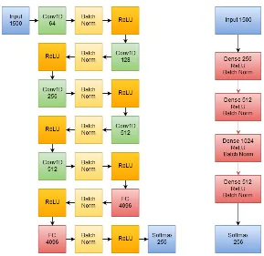
The authors propose a couple of neural network architectures namedMLP best
andCNN best. The latter is a variation of a network called VGG16 [32] with changes on input and classification layers. The former is an MLP architecture with 4 hidden layers, 200 nodes each. These architectures have been taken in the present study as a replay baseline on this dataset. The authors come up to the conclusion that MLP architecture performs better than CNN except in presence of random shifting where CNN prevails.
Both in the reference paper and in the present replica, the results produce a apparently low level of accuracy (0.007, random guessing accuracy is 0.004). Despite the intuitive idea that the model does not learn anything at all, accept-able results are obtained in terms of ranking. The explanation hypothesis is that despite performing extremely poor in terms of single trace matching, the model achieves to approximate the distribution enough for allowing multiple traces matching. More theoretical research in this domain is required to drive some concrete conclusions.
Investigating further into the code provided by the authors it can be seen that despite the rigorous use of 10-fold for choosing the hyperparameters, they do not use the validation set for checking during the training. Moreover, they do not implement any form of regularization either.
3.2
Bias-variance trade-off
During the learning phase we investigated classical methods of network opti-mization. On the one hand some like batch normalization aim at improving the learning capabilities with variance reduction. But on the other hand some others generate variance in order to fight against overfitting: dropout, regularization, data augmentation. Our first intention on the provided model was to fight the overfit. Empirically, in order to go to the extreme, with given complexity of the network it is possible to achieve 100% accuracy on the train set while reducing the learning rate to 10−5. But the difficulty is to find a satisfactory trade-off between these antagonist effects.
Figure 1:Left: Base Convolutional architecture; Right: Base MLP Architecture
rigorous explanation of this phenomenon. While Batch Normalization reduces the internal variance, Dropout with its stochastic properties does exactly the opposite, inducing randomness in weights distribution.
We also tested regularizations based on bothL1 andL2 norms. During the optimization, the best results were achieved usingL2regularization in combina-tion with Batch Normalizacombina-tion. This showed better performance than Dropout. Data augmentation has also been experienced as a regularization tool. To conduct our experiment, we used 2 control groups: original dataset and dataset with 30,000 training examples. For the remaining (augmented) data we took 30,000 original curves and oversample 20,000 from it. We used shifting by some
3.3
Results on target A
On target A data the key has been retrieved in 42 challenge traces using much smaller MLP network with only one hidden layer and 512 units,L2 regulariza-tion and Batch Normalizaregulariza-tion. This validates the replica of the reference paper that left room for improvement since the authors needed around 200 challenges to succeed.
3.3.1 Jittering:
Then the jittering protection has been simulated with random shifting on the signals in order to test the CNN architecture. Due to the presence of translation invariance properties of convolutional networks, the model is able to find the information even when it is shifted randomly as long as it is still present in a vector. For the same reason, the MLP architecture was not tested at all. The results confirm that the performances are not particularly influenced. In the extreme cases (max shift 500 samples) it takes more time to converge and also requires to decrease the learning rate more often during the training. But a mean rank of 20 is still achievable.
Another protection test consisted in rotating randomly by 0 to 3 clock cycles, the 12 last clock cycle patterns (amongst 20) where the masked variable is supposed to be. Contrary to expectations the MLP architecture performed quite well reaching rank 1 in only 46 traces, quicker than non-optimized CNN that needed 250.
3.4
Results on target B
On target B the key could be retrieved in 150 challenge traces with CNN archi-tecture.
3.4.1 Jittering:
In non-masked case (unmasking with the knowledge of the mask) the observable level of accuracy is above 0.95 for all cases which allows single trace matching. If artifical jittering is injected the accuracy is lightly lowered and the fitting time increased due to the higher dimensionality of the traces. In the end the same trend can be observed and the model resists to the shifting.
3.4.2 Shuffling:
Figure 2: Validation accuracy during training CNN on electromagnetic traces with random shifting [0,500].
N Traces N Epochs Accuracy 100,000 50 0.32 500,000 40 0.51 1000,000 40 0.55
Table 2: Test set accuracy on using shuffling protection mechanism on un-masked target B
By construction the shuffling protection demands the translation invariance properties from the classifier since each addressed byte is handled each time at a random position amongst 16. This excluded a MLP based classifier and CNN architecture came up as a natural choice.
With ”unlimited” data (practically 106 curves were available for learning) the effect of continuous data augmentation on attack efficiency could be studied. Since the training process was taking a considerable amount of time ( 3h per epoch using 950,000 training set) only extreme values of the set size, mainly 50,000, 500,000, 1000,000 were tested. The latter was also use to repeat the experiment against another byte as a target. The results are provided in Table 2.
With a CNN architecture 0.55 accuracy is achieved on 95,000 learning traces. The key can be recovered in a few traces (2 for the specific used value, but all of them were not tested).
testing with probability 13. With 500,000, 2 challenge traces were enough inthe worst case. This clearly confirms that CNN works quite well when the leakage does not occur at a fixed time position. From a defensive point of view, in absence of masking, shuffling only is not a sufficient protection.
3.5
Lessons drawn
A general lesson drawn confirms the DL capability of attacking masked imple-mentations of AES SBox with even less challenge traces than in the reference paper. Regarding the neural network architectures a first lesson concerns the interest of CNN versus MLP when time translation invariance is needed, that is in presence of jittering or shuffling. However MLP remains more effective in any other cases. A second observation regards the dimensional hypermaram-eters: roughly speaking, for a given amount of trainable parameters (imposed by computational ressources), deep networks with more layers work better than broad ones (with more neurons per layer but less layers).
Some other practical lessons deduced from DL techniques implementation regard data preprocessing and optimization.
3.5.1 Data Preprocessing
Data preprocessing seems to play a key role in performing a successful attack. There are two important issues: normalization and outliers detection. Nor-malization refers to centering and rescaling the observation Xi, as classically done in statistics with empirical mean T and standard deviation σ through :
Xnorm
i = (Xi−T)/σ. The importance of scaling for deep neural networks is a known fact in machine learning literature [28]. Applied to side channel analysis this has a crucial effect of the classifier capacity. Several experiments were conducted in order to find the better data preprocessing techniques (no preprocessing at all, only mean, only standart L2 normalization). The best per-formance on all datasets was achieved using the described approach. Moreover, when using relatively small datasets (on target A) the particular values of em-pirical mean affect the performance of the model. Assuming that the emem-pirical mean is hard to estimate in real test phase, the one from the training set were used instead to rescale the test set and achieved the reasonable results.
The drawback of scaling (by σ) in the context of side channel analysis is that model become much more susceptible to outliers when using rank as a metric. Outliers come from hardware glitches during the signal acquisition. When using rank as a principal metric, outliers aggravate the result significantly with particularly distant predictions. A favor can be given to the the predictions which are closer to true class more than those that are more distant.
3.5.2 Achieving optimal learning rate
means of increasing the capacity of the model. Since there are multiple ways to achieve the same result from the point of view of the model complexity, there is no robust methodology on how to select the best (apart of grid/random search). The problem is not trivial. The tricks explained hereafter for optimizing the hyperparameters of our model are derived from the methodological advices found in [15].
During the study, it turned out that the learning rate is by far the most important machine learning parameter. It is quite difficult to preset it prop-erly. Moreover, the definition of good learning rate changes during the training. Intuitively, we would like to have high learning rate in the early stages of train-ing and lower learntrain-ing rate when reachtrain-ing some saddle points. To achieve this result several methods can be used: first start by using ADADELTA proposed by [37] which is an automatic way to adjust the learning rate. While observing improvement as compared to standard Batch Gradient Descent, one also notice the oscillations of loss during latter stages of training, incriminating a too high learning rate. The second idea to tackle this problem was to use learning rate schedule, i.e. decrease the learning rate after some number of epochs. The prob-lem here is that since the topology of the loss function is unknown, it is hard to decide when to apply this decrease a priori. Therefore, this method can be used only in case of well-known topology, where the saddle points are detected and the learning rate schedule triggered appropriately. FinallyReduceLROnPlateau
callback fromKeraslibrary was used. This heuristic consists in reducing learn-ing rate once there is no improvement observed durlearn-ing some number of epochs. Empirically, this helps to reduce the oscillations during the late stages of training and significantly increase the final accuracy.
Also, in order to reduce overfitting and to use computational resources more efficiently , early stopping was applied. It consists in stopping the training while there is no improvement in validation loss during some number of epochs. The combination of both early stopping and learning rate reduction showed particularly efficient performance.
4
PCA Improved TA
It is challenging for TA at least too understand how DL succeeds against mask-ing. By the way let’s mention a usual reproach addressed to techniques derived from machine learning: they provide with effective results but do not give any explanation and thus do not help the designer of secure routines. (One can also doubt about the DL capability of achieving a successful attack in real on the field conditions).
4.1
PCA in the masked case
In that point of view the analysis is deemed to failure if the POIs cannot even be identified.
For the class covariance matricesRk, things are somewhat different. As soon as the mask leakage is included into the observation time window, the covari-ance should contain significant non diagonal elements relating the dependence between the mask and the masked variable leakages. To roughly illustrate this statement let us consider a constant valuekmasked with a random masku; be-sides let’s assume a simplistic Hamming weightHW leakage overbbits for both (variance isb/2). Following [12] it can be shown that there exists a correlation between those leakage points.
ρ(HW(u), HW(k⊕u)) = 1−2×HW(k)
b
There are some (second order) remainders of these cross dependences in (PTRkP)−1 if the projection P is based on the global covariance matrix R (which tends to E[Rk] if S = 0). As a consequence the PCA must solve the Eigen problem applied to the covariance matrix (and not toS anymore).
The test is akin to second order analysis in non-profiles SCA. Including the mask leakage in the observation window along with the masked variable may represent a practical issue when thinking that the mask can be initialized far before using it. During profiling this requires refined reverse engineering of the process and possibly alignment tools. The random mask generator should also entail variance within the signal but not correlated to any available data.
If all required conditions are fulfilled, masking impacts also the matching phase. Even though the acquisition is supposed free of measurement noise, single trace matching is utopic because every value will appear concealed by any possible masks. So it is expected that the matching can succeed only statistically with multiple presentations.
4.2
Normalization
Normalization Mask Mask + CC shuffling
No 50 2000
Yes 45 200
Table 3: TA-PCA matching results on target A: the table displays the amount of candidates required for reaching rank 1 with likelihood aggregation. Single traces average ranking remains beyond 100 or around 60 after normalization.
4.3
TA results on target A
The results of TA-PCA on target A are summarized in the following table 3. 45,000 traces were used for profiling and 5000 for matching. They prove that the method also works in the masked case as DL techniques even when the last clock cycles are slightly shuffled. Conversely it completely fails against random jittering, unlike DL-CNN. Normalization also brings some substantial benefit but it requires more principal components (less than 10 up to 60 here).
4.4
TA results on target B
When applied to target B traces as such, TA-PCA failed for any number of principal components. After normalization (taking advantage of the privileged condition in this study), the ranking converged down to 1 after 4500 candidate traces. The performance is much lower than the 150 of DL. However convergence could be accelerated below 1000 by the discarding of outliers (which was used by DL).
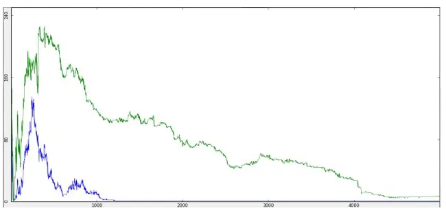
Figure 3: Average trace (up) and first 3 Eigen vectors of target B: without normalization (left), with normalization (right). Normalization kills the phys-ical interpretation whereas the 2 regions of interest mask/masked are visible otherwise.
4.5
Synthesis of the results
Figure 4: Ranking convergence with and without normalization.
proved that supervised attacks could be successful however. The previous results show that TA can also succeed provided PCA is applied first to the covariance matrixR, in order to exploit cross dependences for unmasking. As a matter of fact PCA seems to be the success condition. Possibly it is implicitly included within DL neural networks across all the multilinear combinations implemented. Beware that if the principal components of R are necessary to identify the significant POIs at 2ndorder, the hypotheses discrimination during matching relies on the classes covariancesRk and not anymore on the templatesTk them-selves, since masking equalizes them all. It would not make any sense either to use the common covariance R in the likelihood formula as often done for non masked situations.
Knowing that unlike CNN-DL, TA remains dependent on the good alignment of traces, it appeared also that the improved TA was able to break implemen-tation protected with combined masking and shuffling. This sounds natural since shuffling does not misalign the signals. As counterpart more challenges are necessary in test phase, but (still inspired but DL techniques) the normal-ization seems to bring substantial optimnormal-ization allowing a quicker convergence of multiple traces matching.
5
Results against static targets
value of the secret can be candidated with around 390 traces if all 100,000 challenges are submitted.
Case C is the most simplistic. The leakage is analysed through power. Sub-stantial correlation up to 0.6 can be observed withHW(Kj) andHW(Kj⊕j) wherej is the byte index. A couple of POI with different leakage params and reasonable noise make one of the most favorable situation for TA.
Case D is more realistic since it is implemented on a recent chip for smart card. The transfer is performed with 32 bit words. But the words are set in different experiments with either 8 or 16 or 32 random bits (unused bits are 0). The correlation rate of EM leakage is around 0.15 with the Hamming weight of the word (no matter the number of used bits). Alignment is perfect and optionally shuffling can be activated.
5.1
TA on target C
Average ranking results (1-256) of classical TA are summarized in figure 6 show-ing the benefit of likelihood aggregation when compared with sshow-ingle trace match-ing. It is to be noticed that a dimensionality reduction to 40 POI is performed here classically through SNR/SOST and no PCA. Besides it is remarkable that prenormalization proves to have strictly no effect on the values ranking even if combined with PCA.
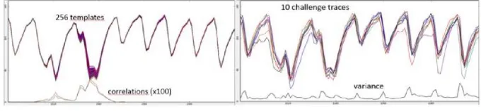
Figure 5: Templates with correlation (left) and raw signals (right).
5.2
Comparison with DL-MLP on target C
A MLP test has been conducted on the same dataset with comparable set-up as used for TA: 900,000 traces for learning, 100,000 for testing; same 40 POIs. The neural network is simple with only 3 layers of 256 neurons each.
Comparative results of classical TA versus DL-MLP are summarized in table 4 showing that both approaches perform well with an advantage for the MLP which converges faster.
Figure 6: TA ranking (1-256 restricted to 1-101) vs values (0:255): aggregated (left) and single traces rank averages (right). Multiplying the number of chal-lenge traces per values improves the ranking but converges after a while.
5.2.1 Is single trace matching utopic?
As soon as even a little noise is involved in measurement it is hard for the right solution to reach rank 1 in one shot (even for MLP). Likelihood integration of aggregated challenges (which is equivalent to challenges averaging) remains the only solution for extracting the secret out of noise (or reducing the noise).
5.2.2 Surjective leakage.
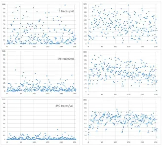
Figure 7: DL-MLP ranking (1-256 restricted to 1-101) vs values (0:255): aggre-gating 8, 39 and 390 challenges per value (top-down).
combinations of POIs (e.g. additional Hamming distances) and unbalanced bits weights that disperse the templates over more than 9 levels. This explains why some values seem to perform better than others. All of them should be calibrated in test phase but also during profiling. Displaying all the templates gives already a qualitative view of the scattering better than SNR/SOST which are statistics. The grouping status or distinguishability power can be represented by the matrix of pairwise weighted distancesδij = (Ti−Tj)TR−1(Ti−Tj).
5.3
TA on target D
N Traces Nb traces /val TA avg rank (aggr) MLP avg rank (aggr)
2,000 8 24 2.16
10,000 39 8.9 1.24
100,000 390 3.5 1.07
Table 4: Comparative average results on target C after aggregation: MLP needs less challenges to performs better.
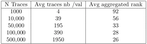
N Traces Avg traces nb /val Avg aggregated rank
1000 4 92
10,000 39 56
50,000 195 33
100,000 390 28
500,000 1950 26
Table 5: TA matching average results on target D (8 bit case): over all values ranking after likelihood aggregation are to be compared versus single traces average ranking 110 which is not far from 128.5 which means ”matching at random”.
PCA (onS).
5.4
Extension beyond 8 bits
Experiment phase Selection byte Other bytes Comment Profiling Random Random
Matching on learning set Fixed Random All values calibrated Matching Fixed Fixed Real test attack Table 6: Analysis situations with leaking words larger than the selection byte
been addressed by Wagner et al. [36] against the round key registers of a hardware DES (exclusive OR input). The leakage is due to 48 bits that flip at each round update. The authors noticed that some special transitions, called ”rings”, between the same key bits are repeated from round to round. They implemented the profiling on 8 bits among 48 and then played several variants of the TA with manysingle trace matchingsover a lot of keys. They showed that some information can be gleaned on the key. But the assessment of the guessing entropy remains on debate.
5.4.1 Implementation issues
Following this example we have implemented this partial selection operated over a subset and chosen 1 byte amid 4. The question is to know the impact the 24 non selected bits during the learning phase and during the test phase (Partial CPA rate falls from 0.12 down below 0.04 typically). During the learning phase they can be chosen as fixed (set with which value?) or random.
If the non selected bits are fixed at learning they will probably introduce a special bias on the templates which has high chances to differ from the one at matching. In the best case this bias is equivalent to an offset. As a consequence a chosen data strategy can be implemented in learning phase: for instance, for each selection byte, the others could be set to zero. But this approach has high chances to be inconsistent with the test phase (even with normalization).
If the 24 bits vary at random they introduce an average bias on templates and drastically increase the variance of noise (within each class in the TA paradigm). Let’s illustrate that point with a Hamming weight: the variance for 8 bit is 2; for 24 bits it becomes 6. This “data noise” is not present in test phase but the 24 bits have a fixed value.
5.4.2 Target D in 16 and 32 bit cases:
These approaches have been experienced in the present study. First, all data have been chosen randomly for both the profiling (200,000 traces) and the testing (400,000 traces). Having unselected bytes set with random is interesting in terms of calibration (Beware, this makes sense only if the subset used is different from the one used for learning). This must be viewed as best case highly favorable to the attacker: if it fails the attack will fail too forcely. Another advantage is that all possible values of the selected part can be tested. But it is not realistic since the true attack deals with a fully fixed key which cannot benefit from averaging multiple presentations (tab 6). Results per secret value are summarized in figure 8. They behave the same with 16 or 32 bit sized data. Let’s notice that they are the same no matter the POI are selected with classical SNR/SOST or PCA.
Figure 8: Rank vs value presented around 1500 time seach: single trace matching (right) looks like matching at random with average rank around 128 on any value unlike aggregate rank per value (left) which shows high variability (some values work, some others not at all).
A couple of complementary tests have been conducted. In a second step real 32 bit, resp 16 bit fixed keys have been compared 50,000 times each to the same dictionary of templates profiled on one byte only. Ranking goes up beyond 200 in both cases (although the effect of measurement noise has been reduced by 50,000 presentations).
Then in a third step the dynamic target has been simulated on the same set of data. For that purpose the 400,000 challenge values were all artificially aggregated with cross-matching into one single result. This test showed that the ranking could go down to low values, asymtotically to rank 1, but only after at least 200,000 presentations!
5.4.3 Preconclusion
argued that the selection byte can be enlarged beyond 8 bits so as to reduce the variance of non-selected ones. The experience shows that 16 bits partitioning is prohibitive; 10 to 12 is accessible but the implementation becomes tedious and the results remain hazardous. Anyway this is unsignificant in front a 32 bit or larger leakages (as in hardware devices).
The large coding size has a different impact dynamic targets that can still benefit from the challenges aggregation since there still remains values which perform not so bad. Obviously integration remains the only solution against noise.
5.5
DL method on target D
5.5.1 8 bit case
The basic 8 bit case has been addressed with DL-MLP on the basis of 500,000 traces for learning and 50,000 for testing, all of them with random byte. So all secret bytes could be tested with around 200 submissions for each. In learning phase overfitting needs L2 regularization. The testing phase produces results similar as TA. Single trace matching does not work at all. Aggregation is neces-sary to gain some information : then all values do not perform the same but an average ranking of 28 can be achieved, which is barely better than TA results (33 with 50,000 challenges in table 5).
Then an attempt has been done to play a real attack against a fixed di-versified 8 bytes key (transferred 50,000 times). As expected the bytes do not perform the same at all : one byte is ranked below 10, another beyond 240 and several others around 100 ! Surprisingly the ranks do not match with the ones expected from the previous test. This shows that the portability remains a hard point even on the same device.
5.5.2 16 bit case
The same test against the 16 bit implementation has been tried also. In that case the training phase completely fails to provide with significant accuracy because of too much randomness. Finally the test phase is not even worth being launched. This means that there exist some situations where the learning phase can early conclude that the attack is deemed to failure without implementing the challenge phase. This represents a practical interest for testing purpose.
5.6
Lessons drawn
quite easily whereas some others cannot be distinguished at all. On average the overall yield is poor.
The effect of coding size is confirmed as merely dissuasive for supervised attacks (as long as integration remains impossible). When the selection data is smaller than the manipulated words, the test phase looks like random challenge. So far even DL techniques fail because non selected bits pollute the learning phase with intense randomness and introduce constant deviations at matching against which averaging is powerless. Larger words are more secure. This conclusion is rather reassuring for designers who have to protect data transfers for instance. Beware however not to set the non selected bits with random data in testing phase : this is not masking but just additive noise which effect can be mitigated with averaging.
6
Synthesis
6.1
Supervised attacks can defeat masked encryption
TA can succeed against masked encryptions and performs not so bad when com-pared with DL techniques. For TA the condition is to work on PCA subspaces computed from the global covariance matrix for 2nd order POI identification and exploit of the non diagonal elements of the classes covariance matrices. It is possible that DL techniques proceed the same implicitly as multiple linear com-binations are performed within the networks. This has practical consequences during profiling. When using SNR/SOST indicators for raw data dimensionality reduction, bias peaks are erased by the masking : this does not necessarily mean that matching will fail. The SNR/SOST must be recomputed after projection onto the Eigen vectors subspace in presence of masking protection: this helps the truncation to retained principal components.
This conclusion stems from tests conducted against masked encryption which is seen as a dynamic target (varying mask in test phase) and considered as rel-evant for supervised attacks mainly by the research community. This situation is much less encountered on the field where cryptographic implementations are much more protected against DPA/CPA.
6.2
Static targets offer good resistance
As traditional targets of TA, the static data manipulations (e.g. data transfers) are more suited to supervised analyses even on real products. This study shows that they are most often difficult to attack with DL and TA techniques. The main explanation resides in a too surjective leakage that thwarts the templates distinguishing even though the noise is removed. A few secret values can be inferred quite well whereas most of the others do not work at all.
within the leaking word, beside the selection ones. Coding secrets over large words seems to be merely dissuasive even to DL methods, at least so far.
6.3
The effect of cross-matching
A basic consequence of the previous points is that dynamic targets, even when protected with masking, are intrinsically more vulnerable that the static ones. By the way, it can be deduced that if encryption is not masked the weakness is even worse. The reason for such a vulnerability is the presence of the varying message in the test data set. It allows the so-called cross-matching
that redirects -through the K⊕M operation- the challenges traces towards easily distinguishable classes even if there are only a few. Amongst the varying messages there is always one to hit such a class and make the right guess stand out. A condition for this is that many challenges are necessary to aggregate the corresponding likelihoods. Regardless of noise, single trace matching looks utopic especially in the masked case.
6.4
Residual case: masked static targets
Among the different use cases considered so far, there is a residual situation concerning static targets protected with random masking. For example it is often encountered during key scheduling within SK block ciphers where the key is hidden with its own random mask before being combined with message material. One could devise that the presence of the random mask reintroduces some variability into the leakage during the matching test as the message does in encryption.
We have experienced it with TA. We just had to replay the tests of dynamic targets A and B without cross-matching aggregation. The cryptographic vari-able are simply viewed as transferred data, but concealed with a random mask. The results of ranking for each (8 bit) value, look like those of figure 8. A few values perform not so bad. But the average rank over every values is 55 on tar-get A (around 20 challenges per value) and 92 on tartar-get B (200 challenges per value). When compared with the aggregated case (cross-matching) the conver-gence curves leave no doubt about the unfeasibility of the attack: they merely kill any chance of success even though the amount of challenges were increased. There is still a remaining floor to ranking as long as cross-matching aggregation cannot help circumventing the leakage surjectivity.
This result confirms that adding a masking protection does not decrease the security of data transfers. This would sound paradoxical. As an outcome table 7 can be derived to summarize the intrinsic resistance of the different use cases encountered in SK implementations against DL and TA supervised attacks.
6.5
Protection of static targets
Leakage observation Type of problem Resistance
L(SBox[K⊕M]) Encryption Very low
L(u),L(SBox[K⊕M]⊕u) Masked encryption Low
L(K) Secrecy transfer Possibly high
L(u),L(K) Masked key schedule Very high
Table 7: Typical targets of supervised attacks and their intrinsic resistance.
software designers. In case of bijective leakage (and low noise), some protections are needed. Since DL techniques such as CNN can still perform through slight jittering and shuffling, it is recommended to implement additional protections as large coding sizes (preferably for data transfers) and/or random masking (key schedule). Beware that random padding (of unsused bit within a large word) is not theoretically sufficient because aggregation can potentially cancel its effect with statistical integration.
6.6
Protection of dynamic targets
In front of supervised attacks (including TA), the main weakness of -even masked- encryption resides in the presence of the message in test/matching phase which circumvents the difficulty of surjective leakages thanks to cross-matching. This variability has a second consequence in case of large coding size (which has not been fully tested ondynamic targetsduring this study). Indeed it has been seen on astatic case that if the non selected data vary ran-domly in test phase, the rank can converge down to low values if a large amount of challenge traces are aggregated. So for encryption large words are not to be considered as an absolute protection as such, just as an efficient noise additioner. Besides DL-CNN still operate through jittering and shuffling provided these are not too strong. So what can a programmer do in front of this darkened picture of possible protections? As a matter of fact the situation is well known in the context of DPA/CPA attacks. A first recipe consists in pushing the countermeasures to their maximum. Further robust cryptographic libraries use to implement complex combinations of the abovementioned types of protections. When two or three of them are present the analysis becomes highly difficult. In the worst cases it remains theoretically possible but demands a prohibitive number of exposures, incompatible with the application context.
6.7
DL versus TA
This concurrent study shows that DL techniques perform better than TA when the attack is feasible, thanks to a much bigger computational effort. But TA competes honorably even against masked encryption. However both TA and DL fail against tough targets as example D.
preprocessing and extraction step. The method used for feeding the model with relevant signals (mask + masked variable leakages) requires the same signal pre-processing and profiling methods used for TA (which demands alignement). A special hard point also regards the possibility of working with long signals: DL public libraries quickly meet memory limitations in such situations. In other words DL techniques would face the highest difficulties without the initial re-verse engineering steps of classical approaches. This mitigates their benefit, knowing that TA can also be improved on its side with PCA and normalization. A significant advantage of DL-CNN is the capability of working with mis-aligned data. This feature is of highest importance against the desynchronizing countermeasures. It deserves being challenged and pushed to the limits on tougher examples with large jitter combined with shuffling. An original point is that the filters responses convolved with the traces are not prior defined (they are initialized with random!). But they are fully part of the model fit-ting optimization process, including the hypotheses separation. They behave like adaptative filters. But they cannot be reproduced as preprocessing because they do not look like the operations usually conducted by alignment methods.
7
Conclusions
The advent of DL techniques in the scope of side-channel attacks does not really appear as a major breakthrough that would severely jeopardize every existing implementations. But it is an opportunity to reconsider classical learning in a different way. Comparable performances can be achieved with TA improved by well-known preprocessing such as PCA and normalization. Similar failures are also observed with both approaches in front of difficult use cases. This com-parative study explains why some protections such as masking can be defeated whereas DL algorithms are often seen as mysterious black boxes.
Without speaking of a new momentum, DL methods (beyond their friendly-ness, public availability) are worth being further challenged in front of tougher targets since they provide with special capabilities of thwarting some protec-tions like desynchronization. As the computational power is getting less and less costly an interesting axis regards the capability of treating the reverse en-gineering and signal preprocessing steps which require a lot of memory and calculations (CNN). The special hard point of working on different devices be-tween learning and testing phases remains to be addressed. Let’s notice at last that this conclusion is somewhat different when considering PK cryptographic implementations which are always special: DL methods turn out to be very helpful for reverse engineering purpose.
References
[2] C´edric Archambeau, Eric Peeters, F-X Standaert, and J-J Quisquater. Template attacks in principal subspaces. In International Workshop on Cryptographic Hardware and Embedded Systems, pages 1–14. Springer, 2006.
[3] K. Lemke-Rust B. Gierlichs and C. Paar. Template vs. stochastic meth-ods. a performance analysis for side-channel cryptanalysis. InInternational Workshop on Cryptographic Hardware and Embedded Systems, pages 15–29. Springer, 2006.
[4] Ryad Benadjila, Emmanuel Prouff, R´emi Strullu, Eleonora Cagli, and C´ecile Dumas. Study of deep learning techniques for side-channel anal-ysis and introduction to ascad database. 2018.
[5] Eric Brier, Christophe Clavier, and Francis Olivier. Correlation power analysis with a leakage model. InInternational Workshop on Cryptographic Hardware and Embedded Systems, pages 16–29. Springer, 2004.
[6] Eleonora Cagli, C´ecile Dumas, and Emmanuel Prouff. Convolutional neural networks with data augmentation against jitter-based countermeasures. In
International Conference on Cryptographic Hardware and Embedded Sys-tems, pages 45–68. Springer, 2017.
[7] Suresh Chari, Josyula R Rao, and Pankaj Rohatgi. Template attacks. In In-ternational Workshop on Cryptographic Hardware and Embedded Systems, pages 13–28. Springer, 2002.
[8] Marios O Choudary and Markus G Kuhn. Efficient stochastic methods: profiles methods beyond 8 bits.https://eprint.iacr.org/2014/885.pdf, 2014. [9] Marios O Choudary and Markus G Kuhn. Efficient, portable tem-plate attacks. IEEE Transactions on Information Forensics and Security, 13(2):490–501, 2018.
[10] Jean-S´ebastien Coron and Louis Goubin. On boolean and arithmetic mask-ing against differential power analysis. InInternational Workshop on Cryp-tographic Hardware and Embedded Systems, page 231. Springer, 2000. [11] Mathieu Rivain Emmanuel Prouff and R´egis B´evan. Statistical analysis of
second order differential power analysis. In Journal IEEE Trans. Comput-ers, volume 58, pages 799–811. IEEE, 2009.
[12] Fahn and Pearson. Inferential power analysis (ipa): a new class of power attacks. In International Workshop on Cryptographic Hardware and Em-bedded Systems, pages 173–186. Springer, 1999.
[14] Ian Goodfellow, Yoshua Bengio, and Aaron Courville.Deep Learning. MIT Press, 2016.
[15] Gabriel Hospodar, Benedikt Gierlichs, Elke De Mulder, Ingrid Ver-bauwhede, and Joos Vandewalle. Machine learning in side-channel analysis: a first study. Journal of Cryptographic Engineering, 1(4):293, 2011. [16] Sergey Ioffe and Christian Szegedy. Batch normalization: Accelerating
deep network training by reducing internal covariate shift. arXiv preprint arXiv:1502.03167, 2015.
[17] Ian T Jolliffe. Principal component analysis and factor analysis. In Prin-cipal component analysis, pages 115–128. Springer, 1986.
[18] Marc Joye and Francis Olivier. Side-Channel Analysis, pages 571–571. Springer US, Boston, MA, 2005.
[19] Paul Kocher, Joshua Jaffe, and Benjamin Jun. Differential power analysis. In Annual International Cryptology Conference, pages 388–397. Springer, 1999.
[20] Yann LeCun, L´eon Bottou, Yoshua Bengio, and Patrick Haffner. Gradient-based learning applied to document recognition. Proceedings of the IEEE, 86(11):2278–2324, 1998.
[21] Liran Lerman, Gianluca Bontempi, and Olivier Markowitch. Side chan-nel attack: an approach based on machine learning. Center for Advanced Security Research Darmstadt, pages 29–41, 2011.
[22] Liran Lerman, Romain Poussier, Gianluca Bontempi, Olivier Markowitch, and Fran¸cois-Xavier Standaert. Template attacks vs. machine learning re-visited (and the curse of dimensionality in side-channel analysis). In In-ternational Workshop on Constructive Side-Channel Analysis and Secure Design, pages 20–33. Springer, 2015.
[23] Xiang Li, Shuo Chen, Xiaolin Hu, and Jian Yang. Understanding the disharmony between dropout and batch normalization by variance shift.
arXiv preprint arXiv:1801.05134, 2018.
[24] Zdenek Martisanek and Vaclav Zeman. Innovative method of the power analysis. In International Workshop on Cryptographic Hardware and Em-bedded Systems, pages 586–594. Radion Engineering, 2013.
[25] Thomas S. Messerges. Using second-order power analysis to attack dpa resistant software. In International Workshop on Cryptographic Hardware and Embedded Systems, page 238. Springer, 2000.
[27] E. Oswald and S. Mangard. Template attacks on masking - resistance is futile. InCT-RSA, pages 243–256. Springer, 2007.
[28] Jean-Jacques Quisquater and David Samyde. Automatic code recognition for smartcards using a kohonen neural network. InCARDIS, 2002. [29] Karen Simonyan and Andrew Zisserman. Very deep convolutional networks
for large-scale image recognition. arXiv preprint arXiv:1409.1556, 2014. [30] F-X Standaert and C´edric Archambeau. Using subspace-based template
attacks to compare and combine power and electromagnetic information leakages. In International Workshop on Cryptographic Hardware and Em-bedded Systems, pages 411–425. Springer, 2008.
[31] Benjamin Timon. Non-profiled deep learning-based side-channel attacks.
https://eprint.iacr.org/2018/196.pdf, 2018.
[32] K. Lemke W. Schindler and C.Paar. A stochastic model for differential side channel analysis. In International Workshop on Cryptographic Hardware and Embedded Systems, pages 30–46. Springer, 2005.
[33] Mathias Wagner and Stefan Heyse. Single trace template attack on the des round keys of a recent smart card. https://eprint.iacr.org/2017/057.pdf, 2017.
[34] Matthew D Zeiler. Adadelta: an adaptive learning rate method. arXiv preprint arXiv:1212.5701, 2012.
A
Formulation used for template attacks
A binary variableKtakes 2|K|possible integer values denotedk. The time signal
associated to each experiment i handling a value of K is noticed Xi ∈ RN. This vector of N time samples contains the leakage L(f(K)), f(K) being a known cryptographic primitive referred to asselection function. Partitioning the signal vectors according to the values taken byK allows the definition of statistical moments in each class k with population nk: the average Tk (the
template) and the symmetric covariance matrixRk=E[(X−Tk)(X−Tk)T]. This matrix contains the variance of noiseσk2on its diagonal: it represents within each class the random share that does not depend on k (measurement noise, misalignement effects, leakage of other manipulated data). The non diagonal elements represent the potential interdependences between the time samples taken at different instants.
vectors orN×N matrices. They comply with the multivariate Gaussian for-mulation which is convenient (but rather coarse?) for resuming the probability densities with 1st and 2nd order moments.
The paradigm of template attacks is based upon the Bayesian inference where the probability forK to take valuekwhile observingXi (matching/test phase) is considered through Bayes theorem as proportional to the probability density ofXi whenK=k (profiling phase).
p(K=k|Xi) = p(K=k)p(Xi|K=k)
p(Xi)
AssumingK as uniformly distributedp(K=k) = 2−|K|thea priori prob-abilities are not discriminating. In the Gaussian multivariate assumption this leads to the famous basic formula for the likelihood of hypothesis k which is proportional and thus assimilated to the conditional probability:
p(Xi|K=k)≡
1 p
(2π)Ndet(Rk)exp(− 1
2(Xi−Tk) tR−1
k (Xi−Tk))
In practice the formula is not used as such but rather through its logarithm which is named log-likelihood. This is better numerically conditioned and more convenient to aggregate the results when going from single trace matching to multiple traces matching in test phase, when several challenges Xi are sub-mitted. The hypothesis testing procedure just has to add them and look for
ArgmaxK(Pilog(p(Xi|K=k))) over all hypotheses ofK.
The purpose of the profiling phase is twofold. First it has to compute the set (dictionary) of statistical templatesTk andRk for all valueskand additionally the global onesT andR. But this has poor chances of effectiveness if a prealable dimensionality reduction is not performed. It is based on the research of Points Of Interest (POI) within the signal that are supposed to maximize (generate peaks) on the following quadratic indicators called SNR (a leakage to noise more than signal to noise) and SOST (pairwise sum of square T-differences):
SN R= Σnk(Tk−T) 2
Σnkσk2
SOST= ΣkΣl>k(Tk−Tl) 2
σ2 k+σl2
There are several issues encountered at profiling. It has to be done in two steps : one for POI indentification and one for computing the covariance ma-trices reduced to these POI. The task assumes randomly and uniformly chosen dataKfor partitioning the traces. These traces must be numerous for allowing good statistical estimation. Last but not least : the traces must be aligned! For convenience let’s introduce the scatter square matrix:
where the expectation are taken over the classesk (variance of the templates).
S is related to the global covariance matrices by
R=Ek[Rk] +S
Srepresents the inter-classes scattering, that is the share of (co)variance which is related to the selected data (the rest being noise). In case of masking, this matrix tends to 0 just like the scalars SNR and SOST, since all averages should converge towards the same value. They all loose their efficiency. Let’s remark by the way that they disregard the non-diagonal elements of the covariance matrices.
The covariance matrices must also be inverted and their determinant cal-culated. The computational complexity is O(N3), which can quickly become unfeasible in high dimensional spaces. Sometimes they can even become sin-gular. These are good motivations for dimensionality reductions. Choudary et. Kuhn [10] in their 2018 publication propose a solution to matrix inversion, based on the pooled covariance matrix which gives the better estimates of the true covariance matrix.
For matching the challenge traces have to be captured in compatible condi-tions (the portability issue) and mapped over the same POI to keep the compa-rability. Let’s notice a commonly used approximation in test phase: the classes covariancesRk are merely replaced by the global oneR. Well R is sometimes better conditioned for inversion in case of large vectors (without dimensionality reduction) or heterogeneous classes (not equipopulated). But the experience shows that class covariances provide with better discrimination results [3].
B
Principal components analysis
Principal components analysis (PCA) can be used as a preprocessing tool for optimal dimensionality reduction and automatic selection of POIs. Under the condition that all the signals are aligned, PCA implements a linear projection matrixPapplied to vectors and covariance matrices onto the subspace of princi-pal axeswhich result from solving an Eigen problem. The basic question regards on which matrix this underlying Eigen problem must be applied. Basically the first target is the covarianceRbut the authors [2] introduced the scatter square matrixS in order to optimize inter-classes scattering. Furthermore it may also apply to R−1S as a kind of SNR criterion maximizing inter-classes scattering over global scattering and noise (a.k.a Linear Discriminant Analysis LDA).
Without loss of generality let’s work onS for instance and solve the Eigen problem SV = VΛ, where Λ is the diagonal matrix of Eigen values λi, and
V the Eigen vectors that make an orthonormal basis. Λ is to be truncated along its diagonal into Λ0, in order to reduce the dimensionality. The projection
matrix is defined asP =VΛ0Vt. The projective form of the likelihood formula just consists in replacing the covariance by (PtR
kP)−1and the signal/template vectors byPt(X
in projecting the raw tracesPTXiand replaying the whole profiling procedure: the new SNR/SOST will provide with relevant truncation parameter).
Experience shows that the truncation decision to main Eigen vectors as required by PCA is a fuzzy issue and criteria based on relative sums of Eigen values is not really effective. A rule of the thumb can be: N0< N is chosen so that ΣN0λ
i/ΣNλi ≈0.8. In classical cases a dozen components are sufficient. Eventually in classical unmasked cases PCA brings poor benefit when compared with classical methods such as SNR or SOST used for POIs identification.
C
Deep learning in a nutshell
The reader is referred to reference papers [23, 4] for fundamental definitions of DL applied to side-channel analysis. A few basic ones are just reminded here-after. The DL approach is based upon the definition of neural network archi-tectures such as the Multi Layer Perceptron and Convolutional Neural Network designed to solve prediction and classification problems. They are built upon the same basic cell calledneuronwhose output result is a multilinear weighted sum of the N input samples followed by a non-linear activation function.
These architectures contain several layers of neurons each applying a linear combination function to the input vectors (∈ RN), with its specific weights. For classification problems the output layers takes the form of probability vectors
p(K=k|X) (softmax function), typically 256 for 8 bit value inference.
The Multi Layer Perceptron (MLP) is one the oldest network used: it is fully connected in the sense that each layer cell is connected to all the cells of the next layer. The CNN architecture is not fully connected: each neuron is connected to a limited number of other local neurons allowing a convolution integration.
During the learning phase a gradient descent algorithm is used to set the neurons with optimal weights. The minimization criterion is the loss function defined as the distance between the expected known values and the predicted outputs.
A network is not only characterized by its connectivity but also by several dimensionalhyperparametersincluding the learning algoritm settings:
• Number of layers
• Number of neurons per layer
• Size of the batches, that is the number of traces per minimization iteration
• Number of epochs, an epoch being the number of passes over the whole training set
The number of neurons and the amount of layers can be increased to solve more and more complex problems. This is the meaning of the termdeep learn-ing.
In addition to the loss function, the accuracy is used to assess the effective-ness of the network model. The accuracy is defined as the success rate of the prediction. Both the loss and accuracy are computed along during the learning algorithm. But they are to be calibrated over a validation dataset different from the learning dataset. An important challenge regards the so-called overfitting encountered when the network perfectly fits the learning set (learned by heart) but predicts or classifies any new trace very badly. It is assessed by observing a large difference between the loss function and the accuracy evaluated on the validation set. To fix this overfitting issue there exist a variety of techniques:
• Data augmentation consists in artificially increasing the number of input traces during the training.
• Regularization (L1 or L2) constrains the neurons weights within bound-aries in order to avoid algorithmic divergence.
• Drop out consists in removing some neurons at random during the mini-mization in order to increase the variance.
![Figure 2: Validation accuracy during training CNN on electromagnetic traceswith random shifting [0,500].](https://thumb-us.123doks.com/thumbv2/123dok_us/7964200.1321010/12.612.226.385.373.423/figure-validation-accuracy-training-electromagnetic-traceswith-random-shifting.webp)