Classification methods for spatial data representation

(1)

CENTRE FOR

ADV

ANCED

SP

A

TIAL

ANAL

YSIS

W

orking Paper Series

Paper 40

CLASSIFICATION

METHODS FOR

SPATIAL DATA

REPRESENTATION

(2)

Centre for Advanced Spatial Analysis University College London

1-19 Torrington Place Gower Street

London WC1E 6BT

[t] +44 (0) 20 7679 1782 [f] +44 (0) 20 7813 2843 [e] [email protected] [w] www.casa.ucl.ac.uk

http//www.casa.ucl.ac.uk/paper40.pdf

Date: January 2002

ISSN: 1467-1298

Toshihiro Osaragi

Toshihiro Osaragi is an Associate Professor in the Graduate School of Information Science and Engineering at Tokyo Institute of Technology. He was an Academic Visitor at the Centre for Advanced Spatial Analysis from March 2001 to January 2002.

Department of Mechanical and Environmental Informatics Graduate School of Information Science and Engineering Tokyo Institute of Technology

2-12-1 O-okayama, Meguro-ku, Tokyo 152-8552, JAPAN Tel:+81-3-5734-3162 Fax:+81-3-5734-2817

(3)

Classification methods for spatial data representation

Toshihiro OSARAGI

Abstract: It is necessary to classify numerical values of spatial data when

representing them on a map and visually understanding it. In consequence, loss of information from original data is inevitable in the process of this classification. A gate loss of information might lead to a misunderstanding of the nature of original data. In this study, a classification method of spatial data is proposed, in which the loss of information is minimized. Comparing our method with other existing classification methods, some new findings are shown.

Keywords: spatial data, visualization, classification, information loss, AIC (Akaike’s

Information Criterion)

1. Introduction

Our natural interpretation capabilities, originally endowed to human being, are excellent. Thematic maps are therefore very effective to understand spatial distribution of geographical features, since we can use our natural interpretation capabilities to understand colors, patterns, and spatial relevance. This fact simultaneously suggests the importance of expression methods, i.e., how to represent spatial data on a map. That is, according to how creation of the thematic map on a geographic information system is carried out, the characteristics of the original data might be overlooked, or there might be a risk of mistaking judgment about the characteristic which original data has.

(4)

Generally, if we employ a number of classes, the distribution-characteristic of original data can be expressed faithfully. However, if there are too many classes, its legends will become complicated and the map will be difficult to understand; we cannot distinguish delicate color differences. On the other hand, when we only have a few classes, the information such as small vibrating factors or local peaks might be ignored; namely, much information of original data will be lost. Hence, a classification problem has to be discussed from the following viewpoint.

(1) How many classes are necessary to represent the spatial data?

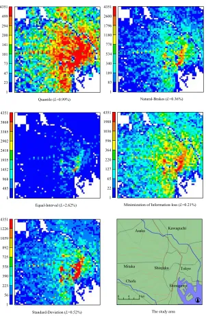
Automatic classification methods are being incorporated in existing geographic information systems. However, the characteristics of the original data might be overlooked, or there might be a risk of mistaking judgment, if we do not have enough knowledge about the classification method as well as the distribution characteristics of the original data. Even if we are using the same number of classes and the same spatial data, we might obtain the quite different maps. A typical example is shown in figure 6. Hence, the following viewpoint is also important for a classification problem.

(2) How the boundary value between each class should be set?

It is true that the classification method to be used depends on the nature of data, and what we want to show about the data. However, more flexible, simple and easy methods are necessary for the non-expert end-users of GIS. In this research, we discuss this primitive and fundamental problem. Hence, the existing classification methods are examined from the viewpoint of information statistics, and we attempt to propose a new classification method for the visualization of spatial data.

As for the former question (1), Umesh (1988) developed an algorithm for achieving efficient classification of data with no a-priori information available about the number of groups. From this a performance index was defined so that minimizing it results in appropriate clustering of the given data.

As for the latter question (2), various methods have been considered and already built in existing geographical information systems. For instance, we have options called Natural-Breaks, Quantile,

Equal-Area, Equal-Interval, Standard-Deviation in a popular GIS software, Arc View. According

(5)

application to actual spatial data in section 4.

Considering the above two fundamental questions, one study that consideres about the cell-size of raster data should be cited. Tamagawa (1987) has analyzed point sampling data by changing the observed spatial-range variously, and proposed a method based on AIC (An Information Criterion) by Akaike (1972 and 1974) to obtain the optimum cell-size. The AIC is a synthetic-measurement considering “model’s fitness” and “model’s simplicity”. This idea is employed to our classification problem.

In this study, the classification method using the evaluation function based on AIC is examined first, and is applied to actual spatial data. Next, based on the consideration about its result, a new classification method based on the minimization of information loss will be proposed. Furthermore, verification of this method is achieved through the examination comparing it with the existing classification methods.

2. Classification Method based on AIC

2.1 Formulation of Classification Method

2.1.1 Discrete variables

Firstly, the spatial data such as point sampling data is discussed. Namely, we focus on the spatial data obtained by counting an attribute value within a certain spatial unit.

First, we denote the variable xi (i= 1, 2, .., n) as an observed value within a certain spatial unit. It is assumed that its value is obtained by distributing the total number of observation within the

whole objective-space, denoted by (=

∑

n₌₁ )

i xi

X , into n space units. That is, the multinomial

probability distribution is assumed here. Next, if the objects are distributed into some spatial units according to the same distributing probability qk (k= 1, 2, .., m), these spatial units should be classified into the same class, denoted by Gk. Therefore, under the condition that the values xi (i= 1, 2, .., n) are observed, the logarithm of Maximum Likelihood Estimates can be written as follows:

∑ ∑

= ∈

+

=

m

k i Gk

k i

k

C

x

q

L

1

log

)

(

ln

, (1)

where C is a constant value. Distribution probability qk has a constraint of

∑

₌₁

=

1

m

(6)

where Nk is the number of spatial units in a class of Gk. The Maximum Likelihood Estimates of qk can be estimated, by using the Lagrange's method of undetermined multiplier considering the constraint of qk, as follows:

k Gk i i k

N

X

x

q

_ˆ

₌

∑

∈ _, ₍₂₎

The number of free parameters qk of this model is m-1. Then, the value of AIC is given by the following equation (Akaike 1972 and 1974), when we classify the original data into m classes:

AIC = -2 [Maximum Likelihood] + 2 [the number of free parameters]

)

1 (

2 ˆ

log

2

1

−

+

−

=

∑∑

= ∈

m

q

x

k m

k i G i

k

, (3)

where the constant term is omitted.

2.1.2 Continuous variables

Spatial data composed of continuous variables can be discussed in the same way. First, the observation value at each place i (i= 1, 2, .., n) is denoted as xi. Next, the parameter common to all observation value is denoted as

θ

₀, and a parameter peculiar to a observation value is

expressed by

θ

_k

(

k

=

1 ,

2 ,

⋅

⋅⋅

,

m

,

∑

m₌₁

=

0 )

k

θ

k .

The number of places which have the same parameter

θ

_k is denoted as Nk

(

₁

N

n

)

m

k k

=

∑

= , and

it is assumed that these places are contained in the same class Gk. That is, the observation value

included in class Gk is assumed to follow the normal distribution (

θ

0

+

θ

k,

2

σ

). Then, the

logarithm likelihood of observed data can be written as follows:

[

]

2 1 2 0 0

2 ln

2 }

,

{

ln

σ

θ

σ

π

θ

∑ ∑

= ∈

−

=

m

k i Gk

k i k

x

n

C

L

, (4)

where, C is a constant.

(7)

as follows, if the undetermined multiplier method of Lagrange is used considering the constraint conditions about

θ

₀ and

θ

_k:

n

N

X

m

k

k k

∑

=

−

=

1

0

ˆ

θ

, (5)

0

ˆ

_θ

θ

=

∑

∈

−

k Gk i

i

k

N

x

, (6)

∑ ∑

∑

= ∈

∈













−

=

m

k i Gk k

Gk i

i

_N

x

n

1

2

1 ˆ

σ

. (7)

Since there is constraint condition about

θ

_k, the number of free parameters of a model is (m+1) in

all. That is, the value of AIC when classifying the data into n classes is given by the following formula, where the constant term is omitted:

)

1 (

2 ˆ

ln

AIC

₌

_n

_σ

2

₊

_m

₊

_.₍₈₎

2.2 Method of boundary setting for classification

We can evaluate each model by comparing values of AIC, which is a synthetic-measurement considering “model’s fitness” and “model’s simplicity”. This is the principal difference between the method we propose and the method proposed by Umesh (1988). Hence, the optimum classification under the condition of the data currently observed can be achieved by minimizing the value of AIC given in the equation (3). Namely, optimum classification can be achieved by the following two steps:

(i) Fix the number of classes m, and search the boundary value of optimum classification, which minimize the value of AIC.

(ii) Repeat the above process by changing the number of classes m one by one, and search the number of classes m that gives the minimal value of AIC.

(8)

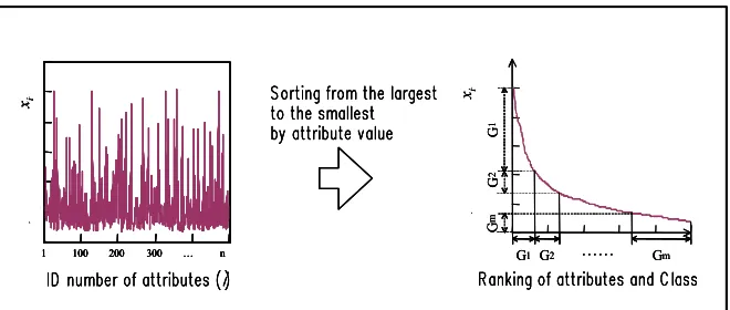
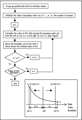
The problem of setting the boundary values of classification will become equivalent to the problem of setting the ranks of boundary values, if the data is sorted in the order of its attribute values (see figure 1). The rank of boundary value is hereafter called "boundary-rank", and a possible procedure of setting the boundary-rank is shown in figure 2. In the following discussion, we consider the condition that the number of class m is fixed for simplicity. The procedure given by figure 2 is described as the following four processes:

(1) Make a group of the spatial units, if their values show a tie.

(2) Set up the initial boundary-rank of (m-1) classes, and consider them as initial values.

(3) Calculate a value of AIC by moving a boundary-rank up or down, and set the boundary-rank so that the value of AIC becomes minimum.

(4) Repeat the above operation until the value of AIC does not decrease.

……

G1G2 Gm

G

1

G

2

G

m

xi

1 100 200 300 … n

xi

……

G1G2 Gm

G

1

G

2

G

m

xi

……

G1G2 Gm

G

1

G

2

G

m

xi

1 100 200 300 … n

xi

1 100 200 300 … n 1 100 200 300 … n 1 100 200 300 … n

xi

(9)

r(k) r*

k=k+1

k=1 Yes

Yes

No No

r(k)

R1=r(k-1)-1 R2=r(k+1)-1

k

k< m

r(k), k=1,…,m m

r(k) r(k+1)

R1=r(k-1)+1

r(k-1)

R2=r(k-1)+1

Gk

Gk-1

r(k) r*

k=k+1

k=1 Yes

Yes

No No

r(k)

R1=r(k-1)-1 R2=r(k+1)-1

k

k< m

r(k), k=1,…,m m

r(k) r(k+1)

R1=r(k-1)+1

r(k-1)

R2=r(k-1)+1

Gk

Gk-1

r(k) r(k+1)

R1=r(k-1)+1

r(k-1)

R2=r(k-1)+1

Gk

Gk-1

Figure 2: Algorithm for minimizing the value of AIC

(10)

- Less risk of local minimum - Consume time to converge

- Converge in short time - Risk of local minimum

- Less risk of local minimum - Consume time to converge

- Converge in short time - Risk of local minimum

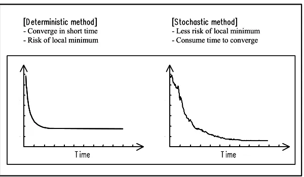
Figure 3: Comparison of deterministic method and stochastic method in the minimization process of AIC

According to our experiments using actual data, we can obtain quasi-optimum boundary-rank that gives almost the minimum value of AIC, if the process of minimization is performed several times by changing the initial boundary-rank. The above method (the deterministic method) does not produce any major practically problem, from the author’s experience.

2.3 Application to Actual Data

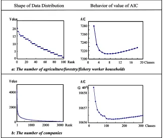
The above method is first applied to the raster data, Digital Mesh Statistic compiled by Statistic

Bureau & Statistic Center of Japan, and the result is shown in figure 4-a. The data source is

"agriculture/forestry/fishery worker households, 1989 Population Census". The cell-size is about 1 km by 1 km, and the number of cells is 100. Figure 4-a shows us that the value of AIC is minimum when the number of classes is seven. Hence, we can say that optimum classification has been achieved from a statistical viewpoint.

Next, this method is applied to the same kind of raster data as "the number of companies, 1994

Establishment and Enterprise Census". The cell-size is about 500 m by 500 m, and the number

(11)

the values of AIC. Furthermore, much time is required to calculate an optimum solution when many classes are considered. Therefore, we cannot call it a realistic classification method.

Considering the above discussion, it may be more realistic to examine only step (ii) described in section 2.2, that is, to examine how we should set up the suitable boundary-rank by fixing the number of classes. As for step (i), GIS users should set up a-priori the number of classes to be employed according to their demands.

Behavior of value of AIC Shape of Data Distribution

a: The number of agriculture/forestry/fishery worker households

b: The number of companies

1 1000 2000 3000 Rank

0 2000 4000 0 5 10 15 20

0 20 40 60 80 100 Rank 7200

7220 7240 7260 7280

0 4 8 12 16 20 Classes

0 100 200 300 Classes

10656 10657 10658

( 103₎

Behavior of value of AIC Shape of Data Distribution

a: The number of agriculture/forestry/fishery worker households

b: The number of companies

1 1000 2000 3000 Rank

0 2000 4000

1 1000 2000 3000 Rank

0 2000 4000 0 5 10 15 20

0 20 40 60 80 100 Rank

0 5 10 15 20

0 20 40 60 80 100 Rank 7200

7220 7240 7260 7280

0 4 8 12 16 20 Classes

7200 7220 7240 7260 7280

0 4 8 12 16 20 Classes

0 100 200 300 Classes

10656 10657 10658

( 103₎

0 100 200 300 Classes

10656 10657 10658

( 103₎

Figure 4: Shapes of data distribution and behavior of the vale of AIC in minimization process

3. Classification Method based on Minimization of Information Loss

(12)

their strategy to our classification problem. In the following, we define the information loss caused by classification first.

We define the averaged information, denoted by I0, for spatial data obtained by counting an attribute value within a certain spatial unit as follows:

∑

=

i

p

I

0

log

, (9)

where

X

x

p

i

=

i . This equation shows the amount of information when any classification is not carried out. That is, equation (9) gives the total information contained in original data, when each value is classified into individual n classes. On the other hand, the averaged information, denoted by I, can be described as follows, when the data is classified into m classes.

∑ ∑

= ∈

=

m

k iGk

k

q

I

1

log

, (10)

where

q

ˆ

k is given by

(

_k

)

Gk i

i

X

N

x

∑

∈

.

The above-mentioned concept about the averaged information of discrete attribute variables can be naturally extended to the case of continuous variables. Denote x as the random variable of continuous data sources, and p(x) as its density function. The averaged information I0 of continuation sources of information can be defined as follows (Minami, 1995).

∫

−∞∞

−

=

p

x

p

x

dx

I

0

(

)

log

2

(

)

(11)

However, actual spatial data are not necessarily obtained in a continuous form, but only the values aggregated in a certain space range are acquired in many cases. Then, in actual calculation, it is considered as follows.

First, the aggregated value in a certain space range

∆

x

i can be expressed by

p

(

x

i

)

∆

x

i (i= 1, 2, ..., n). The averaged information I0 can be defined by the following equation, since the integration range of equation (11) is equivalent to the whole space.

∑

=

∆

−

=

n

i

i i i

i

x

p

x

p

I

1

2

(13)

Here, the value of

p

(

x

i

)

∆

x

i is given by

∑

=

n

k k

i

x

1 .

Consider the case that the whole space is classified into m class divisions. The averaged information I of this case can be defined by the following equation:

∑ ∑

= ∈

∆

−

=

n

i iGk

i k i

k

x

q

x

q

I

1

2

(

)

log

)

(

(13)

The following statistical value calculated using equations (9), (10) or equations (12), (13), is defined as "the ratio of information loss", denoted by L, as follows:

100

0

×

−

=

I

L

(%). (14)

If the value estimated by equation (14) is small enough, we can accept this classification from the viewpoint of information loss. Comparing equation (3) with equation (10) or (13), it turns out that the evaluation measurement of equation (14) is equivalent to the definition of AIC in the case where the number of model’s parameters is not taken into consideration.

The value of AIC is, basically, the relative index used in order to judge the superiority or inferiority of models. Hence, there is no absolute meaning in the value of AIC itself. On the other hand, the ratio L of information loss in equation (14) is an index showing how much information of original data is lost. Therefore, this index L can help us as a reference, when we understand a map drawn using the classified data.

The classification method based on minimization of information loss can be achieved using the equation (14) as an evaluation index. Namely, the optimum classification should be performed according to the procedures described at "2.2 Method of boundary setting for classification ".

4. Comparison of Classification Methods

The above method will be verified through some comparisons with existing classification methods. Before the examinations, the features and capability of existing methods are reviewed briefly.

The Natural Breaks classification method identifies breakpoints by looking for groups and patterns

(14)

optimization in this method, which minimizes the variation within each class (Jenks 1967). The features of the data are divided into classes whose boundaries are set where there are relatively big jumps in the values. As for the Quantile method, each class is assigned the same number of features. This may be misleading because low values are often included in the same class as high values. However, it is the best suited for the data that is linearly distributed, namely, data that does not have disproportionate numbers of features with similar values. In addition, it is suitable when we want to emphasize the relative position of a feature among other features. The Equal

Area method classifies polygon features so that the total area of polygons in each class is

approximately the same. The Equal Interval method divides the range of attribute values into equal sized sub-range. It is useful when we want to emphasize the amount of an attribute value relative to the other values, and ideal for data whose range is already familiar, such as percentage or temperature. Finally, the Standard Deviation method, it shows us the extent to which an attribute’s values diverge from the mean of all the values (ESRI, 1996).

(15)

Table 1: The ratio L of Information-loss: comparison of existing classification methods and a method based on minimization of information-loss

Quantile Equal Equal Standard Natural Minimized Area Interval Deviation Breaks Information-loss

the smallest Information-loss

the second smallest Information-loss

Upper Normal classification

Lower * Round down the first figure / ** Round down the second figure

0.986 0.986 2.615 0.520 0.356 0.210

3.080 3.080 6.323 1.899 0.583 0.332

0.759 0.759 3.100 0.513 0.373 0.219

1.376 1.376 5.461 1.407 0.553 0.280

1.052 1.052 3.282 5.851 1.134 0.837

0.639 0.639 1.233 1.360 0.932 0.562

Industry

Company

Factory

Private Shop ( 10-1₎

Shops

Population (Tokyo 10-1₎

Population (Yoko-hama 10-1₎

Classification Methods Spatial Data

1.323

1.323 5.427 0.915 0.589 0.283

2.945

2.945 6.322 1.866 0.584 0.335

0.975

0.975 2.653 0.505 0.349 0.215

* ** * * * * *

1.315 1.315 2.393 0.515 0.497 0.242

0.792 0.792 3.105 0.507 0.390 0.224

1.058 1.058 3.241 5.875 1.129 0.840

0.645 0.645 1.275 1.415 0.922 0.563

1.194 1.194 2.353 0.708 0.465 0.209

Quantile Equal Equal Standard Natural Minimized Area Interval Deviation Breaks Information-loss

the smallest Information-loss

the second smallest Information-loss

0.986 0.986 2.615 0.520 0.356 0.210

3.080 3.080 6.323 1.899 0.583 0.332

0.759 0.759 3.100 0.513 0.373 0.219

1.376 1.376 5.461 1.407 0.553 0.280

1.052 1.052 3.282 5.851 1.134 0.837

0.639 0.639 1.233 1.360 0.932 0.562

Industry

Company

Factory

Private Shop ( 10-1₎

Shops

Population (Tokyo 10-1₎

Population (Yoko-hama 10-1₎

Classification Methods Spatial Data

1.323

1.323 5.427 0.915 0.589 0.283

2.945

2.945 6.322 1.866 0.584 0.335

0.975

0.975 2.653 0.505 0.349 0.215

* ** * * * * *

1.315 1.315 2.393 0.515 0.497 0.242

0.792 0.792 3.105 0.507 0.390 0.224

1.058 1.058 3.241 5.875 1.129 0.840

0.645 0.645 1.275 1.415 0.922 0.563

1.194 1.194 2.353 0.708 0.465 0.209

(16)

Ratio of Information-loss : L

Distribution of data

0.0 1.0 2.0 3.0 (%)

Minimized Information-loss Natural Breaks Standard Deviation Equal Interval Equal Area Quantile

0.0 1.0 2.0 3.0 (%)

0.0 0.4 0.8 1.2 1.6 (%)

( 10-1₎

0.0 2.0 4.0 6.0 (%)

In du st ry Fa ct or y P opu la ti on (T ok yo ) P op ula tio n( Y oko ha m a) 0 10000 20000 30000

1 400 800 1200

Value Rank 0 400 800 1200

1 2000 4000 6000

Value Rank 0 200 400 600 800

1 2000 4000

Value

Rank

0 2000 4000

1 1000 2000 3000

Value

Rank

( 10-1₎

Ratio of Information-loss : L

Distribution of data

0.0 1.0 2.0 3.0 (%)

0.0 0.4 0.8 1.2 1.6 (%)

( 10-1₎

0.0 2.0 4.0 6.0 (%)

In du st ry Fa ct or y P opu la ti on (T ok yo ) P op ula tio n( Y oko ha m a) 0 10000 20000 30000

1 400 800 1200

Value Rank 0 10000 20000 30000

1 400 800 1200

0 10000 20000 30000

1 400 800 1200

Value Rank Value Rank 0 400 800 1200

1 2000 4000 6000

Value Rank 0 400 800 1200

1 2000 4000 6000

0 400 800 1200

1 2000 4000 6000

Value Rank Value Rank 0 200 400 600 800

1 2000 4000

Value Rank 0 200 400 600 800

1 2000 4000

0 200 400 600 800

1 2000 4000

Value Rank Value Rank 0 2000 4000

1 1000 2000 3000

Value

Rank

0 2000 4000

1 1000 2000 3000

0 2000 4000

1 1000 2000 3000

Value

Rank Value

Rank

( 10-1₎

(17)

4351 499

1 23 47 73 101 141 200 294

Quantile (L=0.99%)

3868

1 485 968 1452 1935 2418 2902 3385 4351

1226

1 56 223 390 558 725 892 1059 4351

Equal-Interval (L=2.62%)

Standard-Deviation (L=0.52%)

2600

1 83 189 340 534 778 1180 1796 4351

1988

1 22 65 127 220 364 596 1036 4351

Natural-Brakes (L=0.36%)

Minimization of Information-loss (L=0.21%)

0 4 8 km

Shinjuku Tokyo

Shinagawa Mitaka

Chofu

Kawaguchi Asaka

The study area

(18)

Table 1 and figure 5 show us that the ratio L of information loss deeply depends on the feature of original data. For example, the Natural-Breaks classification method is effective for the data that has clear breakpoints such as the data "the number of companies". The Natural-Breaks can be acceptable to the variety types of data, since its information loss is comparatively smaller than that of the other methods. However, it should be noted that the Natural-Breaks is unsuitable for the data such as "Yokohama population" which has an unclear breakpoint. As for the

Standard-Deviation classification method, it appears out that there can be a risk of being

accompanied by a large amount of information loss. Furthermore, although it is easy to understand the legends in the Regular-Intervals method, due to the regular intervals in the range of boundary values, it must be recognized that there is a tendency to lose large amounts of information. Moreover, the Quantile method can be excellent for data that shows linear distribution, such as the data "Tokyo population", since its information loss is suppressed. However, in the case of data such as "the number of factories", the Quantile shows quite large information loss.

Considering the above discussion, it is necessary to examine the distribution characteristics of spatial data, in order to determine which classification method should be employed. If this process is neglected, we might have a risk of overlooking the nature of the original data. However, according to the classification method based on the minimization of information loss, we can correspond with flexibility in regards to any spatial data.

5.Summary and conclusions

The classification method based on AIC is proposed in order to grasp the nature of spatial data from the viewpoint of statistical meaning. However, this method is not effective for data with a large number of observations. Then, we proposed another classification method based on the minimization of information loss. This method is examined through the application to actual spatial data and comparing it with the existing classification methods. The results of numerical analysis show the flexibility and validity of the proposed method. However, further considerations regarding the efficient algorithm for minimizing information loss should be discussed.

6. Acknowledgements

(19)

Institute of Technology, for computer-based numerical calculations and drawing figures.

References

Akaike H, 1972, “Information theory and an extension of the maximum likelihood principle” Proceedings of the 2nd International Symposium on Information Theory Eds B N Petron, F Csak (Akademiai kaido, Budapest) pp.267-281

Akaike H, 1974, “A new look at the statistical model identification” IEEE Transactions on Automatic Control AC19, pp.716-723

ESRI, 1996, “ArcView GIS – The Geographic Information System for Everyone”, Environmental Systems Research Institute, USA

Goodchild M F, Guoqing S and Shiren Y, 1992, “Development and test of error model for categorical data”, Int. J. Geographical Information Systems, Vol.6, No.2 pp87-104.

Jenks G F, 1967, “The Data Model Concept in Statistical Mapping" International Yearbook of Cartography, Vol.7, pp.186-190

Roy J R, Batten D F and Lesse P F, 1982, “Minimizing information loss in simple aggregation”, Environment and Planning A, Vol.14, pp.973-980.

Tamagawa H, 1987, “A study on the optimum mesh size in view of the homogeneity of land use ratio”, Papers on City Planning Vol.22, pp.229-234. (in Japanese)