Article
1
Trajectory Tracking between Josephson Junction and
2
Classical Chaotic System Via Iterative Learning Control
3
Chun-Kai Cheng, Paul C.-P. Chao*
4
Institute of Electrical and Control Engineering, National Chaio Tung University, Taiwan;
5
[email protected] (C. K. Cheng); *Correspondence: [email protected];
6
Tel.: +886-3-513-1377
7
8
Abstract:
9
This article addresses the trajectory tracking between two non-identical systems with chaotic
10
properties. We employ the Rossler chaotic and RCL-shunted Josephson junctions model in similar
11
phase space to study trajectory tracking. In order to achieve the goal tracking, we afford two stages
12
to approximate the target tracking. The first stage utilizes the active control technique to transfer
13
the output signal from the RCLs-J system into the quasi-Rossler system. Then next, the RCLs-J
14
system employs the proposed the iterative learning control scheme and the control signal from the
15
drive system to trace the trajectory of Rossler system. The numerical results demonstrate the
16
proposed method and the tracking system is asymptotically stable.
17
18
Keywords: Trajectory; Chaos; Josephson Junction; RCL-shunted; Iterative Learning Control (ILC).
19
20
1. Introduction
21
Chaotic phenomenon was found in the rf-base resistive-capacitive shunted Josephson Junction
22
(RCs-JJ) and the numerical study in three system parameters have been described in [1]. Many
23
studies exhibit the chaotic behavior in superconducting resistive-capacitive-inductance Josephson
24
Junction (RCLs-JJ) [2-4]. The homoclinic, heteroclinic, and super-harmonic bifurcations are
25
respectively excited by parameters has investigated in [5]. The damped pendulum equation can
26
describe the junction behavior and demonstrate the chaotic strange attractor in phase space [6].
27
Synchronization is a significant topic in nonlinear science as the trajectory tracking is essential in
28
studying the chaotic synchronization. A non-linear controller utilized backstepping technique to
29
control bifurcation in the RCLs-J junction has investigated in [7]. The chaos synchronization
30
between two identical systems of RCLs-J junctions investigated in [8-14] in which employ a number
31
of different techniques to design controller, such as using active control in [8], by a common chaos
32
to drive RCLs-J junctions approaching synchronization [9], applying the backstepping in [10, 13],
33
and using time-delay feedback control in [14], respectively. In others, the controller design or
34
controlled rule is directly determined by Lyapunov function in [11-12] and the RCLs-J junctions
35
array synchronization in [12]. In most studies, the synchronization systems were described in
36
identical RCLs-J junction systems. In the classical systems, synchronization is not concerned about a
37
superconducting system. Accordingly, in the trajectory tracking study is rarely based on the
38
combination of RCLs-J and classical chaotic systems.
39
This article regards the trajectory tracking between the Rossler chaotic and the RCLs-J systems as
40
the classical chaotic system and the mesoscopic system in the Josephson junctions model. They are
41
almost two different systems to trace trajectory. This paper affords two stages to approximate the
42
goal of trajectory tracking. The first stage utilizes the active control technique [15] to transfer RCLs-J
43
system into the quasi-Rossler system. Next, we propose the iterative learning control law which is
44
the purpose to approach the signals from the identical system by correcting repetition the tolerance
45
according to preceding output information [12]. The RCLs-J system employs the iterative learning
46
control procedure and control signal from the drive system to trace Rossler system. Although, most
47
research of the ILC are designed linear ILC law, few applications are available on two different
48
systems synchronizing.
49
The organization of this article follows: next section is the description of Rossler Chaotic and
50
RCL-Shunted Josephson Junction System. The third section is to demonstrate the simulation results
51
in figures by designing example and investigating to employ the proposed learning control law into
52
the RCLs-J system to trace the path of the Rossler system. Finally, this paper points out the
53
applications in the future and conclusion.
54
2. The description of Rossler Chaotic and RCL-Shunted Josephson Junction System
55
2.1. System Description and Transformation
56
The Rossler chaotic system has initial condition X0 is drive system in general form as
57
̇ = + =
0 −1 −1
1 0
0 0 −
+ 0
0 (1).
58
The variable = [ ] is the state vector. The RCL-shunted Josephson Junction can be
59
presented by eq. (2) with initial conditions Y0 = [0 0 0]T as
60
̇ = + ( ) + ( ), (2).
61
The parameters in the eq. (2) defined = [ ] , and
62
=
0 1 0
0 −( )
0 −
, = 0
0
, ( ( )) = − sin( ). (3)
63
There is a function ( ) in eq. (3), and given by
64
( ) = 0.366 as | | > 2.9
0.061 as | | ≤ 2.9, (4).
65
The iterative number k in system (2) is the number to employee the iterative learning control law
66
(ILC) ( )= ( ) ( ) ( ) . Really, ILC rule is a sequence of control input signal for response
67
system as ( )
, ,⋯.
68
The system (1) and system (2) are almost not identical nonlinear systems from the trajectory of them
69
in Figure 1. The nonlinear system (2) should be transferred to the quasi-Rossler system to track the
70
trajectory of the system (1). Therefore, the active control technique [17-18] will be utilized into the
71
system (2).
72
According to the active control technique, the description of the system (2) and dynamical
73
transformation between the drive (1) and responsesystem (2) show respectively as
= = − −
− (5)
75
̇ =
̇
̇
̇
= ̇ − ̇ ̇ − ̇ ̇ − ̇
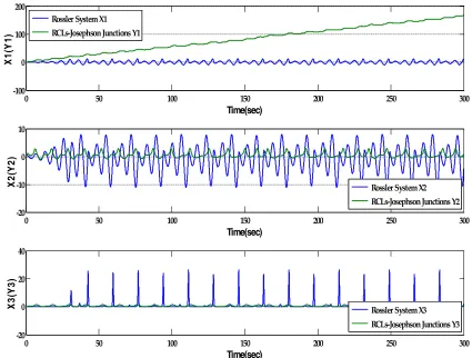
=
⎣ ⎢ ⎢
⎡ + 2 +
( ) + + [ − sin( )] − − + ( ) −
− + ( − ) − − − ⎦⎥
⎥ ⎤
+ (6)
76
The [ ] in eq. (6) is the active control function to eliminate the terms in which have no
77
for the i = a, b, c. As a result, the active control function can be determined as
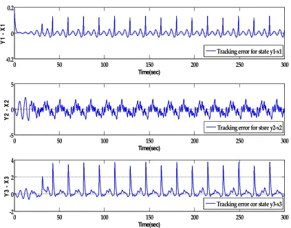
78
=
⎣ ⎢ ⎢
⎡ −2 −
[ − sin( )] + + + ( ) +
( − ) + + + ⎦⎥
⎥ ⎤
+ (7).
79
The [ ] is the error term in active control procedure. Substituting eq. (7) into (6), the
80
eq. (6) became as
81
̇ =
̇
̇
̇
= ( ) −
−
+ (8)
82
The matrix form of eq. (8) is rewritten as
83
̇ =
̇
̇
̇
= + (9)
84
Suppose the matrix A has eigenvalues , , = (−1, −1, −1), the characteristic equations of A
85
are demonstrated as
86
−1 −1 0
0 −1 + ( )
0 −1 +
= (10)
87
The solution of [ ] is
88
=
⎣ ⎢ ⎢
⎡− − 0
0 −(1 − ( ))
0 (1 + ) ⎦⎥
⎥ ⎤
(11)
89
The equation (8) employed eq. (11) and became [ ̇ ̇ ̇ ] = [− − − ] . Substituting eq.
90
(11) and (7) into the RCLs-Josephson Junctions eq. (2) with iterative learning control rule and
91
changing the variable x to y, the system became as
92
̇ =
− − −
+ −
− − +
( )=
0 −1 −1
1 0
0 0 −
+ 0
0 − +
( ) ( ) ( )
(12)
After the active control procedure, the RCLs-Josephson Junctions system became a quasi-Rossler
94
chaotic system such that the trace of trajectory between different systems became identical systems.
95
2.2. Trajectory tracking between of Systems via Iterative Learning Control
96
The RCLs-Josephson Junctions system has now been transferred to the quasi-Rossler chaotical
97
system. The ILC procedure and controll signal from the drive system will be utilized into the
98
response system to track the drive system. When an appropriated ( )
, ,⋯ is found, and the
99
iteration number k is enough, the tracked error dynamical system should be equal to zero, that is
100
̇( )( ) = lim
→∞ ̇ ( ) − ̇ ( ) = 0. The situation of tracking trajectory has changed to two similar systems.
101
In many studies, the synchronization between identical systems employ the control signal from
102
drive system has been studied in [19-21]. Accordingly, The RCLsJ system in eq. (2) utilizing the
103
controlled signals from drive system, x1 and x3, is rewritten as
104
̇ =
̇
̇
̇
= [ − ( ) − sin( ) − ]
( − )
+ ( ) (13).
105
The controlled signals from the Rossler system in eq. (13) is similar to the quasi-Ross system in (12)
106
and the iterative learning control law ( ) which is defined by the error dynamics. The dynamical
107
error system between the Rossler system in (1) and the quasi-Rossler system in (12) exhibit as
108
̇ =
− −
+ −
− +
( ) ( ) ( )
=
0 −1 −1
1 0
0 0 −
+ ( , ) ( ) − +
( ) ( ) ( )
(14)
109
The iterative learning control rule (ILC)in [16, 21] ( ) is defined as
110
( )= ∆( )+ ( ) (15)
111
where the matrix = ( ) ∗ ( ( )) with appropriated 0≤ ≤1, and 1 ≤ < . The
112
is the coefficient matrix of ∆( )=[ ] in (14) and ( ) is the real part of eigenvalue of .
113
When the , , = , , , the term ( , ) ( ) in eq.14 can absorb the [ ] to choose
114
the appropriate matrix M
115
By induction, the expansion of ( ) in eq. (15) wrote as
116
( )= ( ) ( )+ ( ) ∆( )+ ( ) ∆( )+ ⋯ + ∆( )+ ∆( ) (16).
117
2.3. Lyapunov Stability of Systems
118
The equation (6) can be the dynamical error system in the active control procedure. Hence, the
119
Lyapunov function is defined as
120
= ( + + ). (17)
121
The
, , are constant such that ̇ < 0.122
Theorem 1. The Lyapunov function in active control procedure to transfer the RCLs-J system
123
(2) to the quasi-Rossler system (12) can be defined as in eq. (17).
Proof:
125
The equation (17) should be proved the first derivative is negative and the dynamical system is
126
stable at the equilibrium (0, 0, 0). The first derivative of the Lyapunov function is
127
̇ = ( ̇ + ̇ + ̇ ) (18)
128
Substituting eq. (11) into eq. (8) and taking = = = 1, it is easy to show that
129
̇ = −( + + ) ≤ (19)
130
□
131
Theorem 2. Let the ( ) is in the eq. (15), the Lyapunov function is defined in the iterative
132
control stage to trace the trajectory of Rossler system as
133
= ( + + ) (20)
134
Proof:
135
Let ( ) be defined as
136
( )= ∆( )+ , ( ) (21)
137
Applying − ( ) to the eq. (14), we can obtain the error dynamics as ̇ = [− − − ] . Let
138
, , = , , and , , = 1. The Lyapunov function should be as
139
̇ = −( + + ) ≤ (22)
140
which implies eq. (14) employs the iterative learning control law is asymptotical stable at
141
equilibrium.
142
□
143
3. Demonstrating Results by example and discussion
144
To verify the proposed the iterative learning control law, we utilize an example to demonstrate
145
the tracing error and trajectory between the Rossler dynamical system as in (1) with initial state (x10,
146
x20, x30) = (0.2, 0.4, 0.1) and the RCLSJ system in (2) with initial state (y10, y20, y30) = (0, 0, 0),
147
respectively.
148
3.1. Deciding Iterative Control Learning Law by Example
149
The Rossler system in (1) is given as:
150
̇ = + =
0 −1 −1
1 0.2 0
0 0 − 5.7
+ 0 0 0.2
, = 0.2 0.4 0.1
. (23)
151
The RCL-shunted Josephson Junction model in (2) is given by:
152
̇ = + ( ) + ( ), = 00 0
(24)
153
where the parameters in eq. (24) have defined in eq. (3) and (4) in which the values of entries in
154
matrix B are βL = 2.6, βc = 0.707 and the iN = 1.132 is in function ( ) = 1.132 − sin( ), respectively.
The ( )= ( ) ( ) ( ) in the system (24) is ILC rule and defined in eq. (15) to achieve enough
156
small tracking error between the Rossler system and RCLs-J system. The matrices , of eq.
157
(14) and of eq. (15), respectively alternate as
158
, =
1 0 0
0 1 0
0 1
and =
0 1 1
−1 −0.2 0
−1 0 5.7
(25)
159
where the is from Rossler system and matrix is the decomposition of matrix A in eq. (1).
160
The time interval of simulation is from 0 to 300 sec and the minimum time step is 0.01sec. The
161
results and figures in this article utilize the MATLAB to investigate trajectory tracking by the ILC
162
law in eq. (16) in which used program of the Euler method. In the active control procedure,
163
transferring the RCLs-J system to Rossler system employs the Simulink in MATLAB.
164
3.2. Exhibiting Simulation Results and Discussion
165
The fig. 1 and fig. 2 show the time response of state and phase portrait of two distinct systems
166
in which are Rossler and the RCL-shunted Josephson Junctions systems with different initial states,
167
respectively. In fig. 1, the trajectory error between them should be enormous in each state. The fig. 2
168
displays two non-identical phase portraits of two systems and the chaotic behavior of RCLs-J shows
169
in fig. 2(d). To overcome the non-identical trajectory between two systems, the first stage employs
170
the active control to change RCLs-J systems into the quasi-Rossler system form Eq. (5) to Eq. (12).
171
After utilizing the active control technique, the phase portraits of two systems show in the fig. 3 (a),
172
(b), and (c). The new phase portraits of RCLs-J are almost not belonged to original phase portraits
173
and closed to the Rossler system; therefore, we call the new system is the quasi-Rossler system. The
174
time response of each component in the two systems indicated in the fig. 3 (d), (e), (f) in which the
175
paths of Rossler and RCLs_J systems, respectively, are not close to each other.
176
The fig.4 is the tracking error between the Rossler and the quasi-Rossler system which transfers
177
from RCLs-J systems. The vibration of the tracking error has many large amplitudes in the second
178
(y2-x2) and third (y3 -x3) components at the specific moment.
179
The fig. 5 demonstrates the phase portrait of the x1 (y1) and x2 (y2) by utilizing the ILC to track the
180
trajectory. Two trajectories are almost overlapping in fig. 5 in which the phenomena of tracking
181
errors in fig. 6 are also validated. The tracking errors oscillation in fig. 6 are between 0.1408 and
182
-0.1959 for the first tracking error, second one among 0.1434 and -0.4217, and the third tracking
183
error between 0.4784 and -0.8344, respectively.
184
The fig. 7 exhibits the tracking error which is the most different ingredient after using the ILC law
185
and compares the fig. 1 to each other. The lager vibration will always happen at a particular
186
moment such as ti because that the tracking error between two systems became larger at some
187
moments ti. Comparing between fig. 4 and fig. 6, the tracking errors are successful to be suppressed
188
between 0.2 and -0.2 for the first two components and the error of the third component between 0.5
189
and -0.8 by proposing ILC law, and the error is asymptotically stable.
190
4. Conclusions
191
This article has proposed a learning control law to trace the trajectory between two non-identical nonlinear
192
systems and successfully utilized a two-stage approach of combining active control technique and iterative
193
learning control law significantly to inhibit and improve the tracking errors in the numerical results. The
194
work of ILC in the future would be error convergent between multiple non-identical systems and employed
196
encryption and decryption, signal tracking of bio-system, and AI arm.
197
198
Fig. 1 The time response of Rossler system and RCLs-J system
199
(a) Rossler System x1, x2 (d) RCLs-J System y1, y2
0 50 100 150 200 250 300
-100 0 100 200
Time(sec)
X
1
(Y
1
)
0 50 100 150 200 250 300
-20 -10 0 10
Time(sec)
X
2
(Y
2
)
Rossler System X2 RCLs-Josephson Junctions Y2
0 50 100 150 200 250 300
-20 0 20 40
Time(sec)
X
3
(Y
3
)
Rossler System X3 RCLs-Josephson Junctions Y3 Rossler System X1
RCLs-Josephson Junctions Y1
-10 -5 0 5 10 15
-12 -10 -8 -6 -4 -2 0 2 4 6 8
Rossler X1 componnet
R
o
ss
le
r
X
2
c
o
m
p
o
n
n
e
t
0 10 20 30 40 50 60 70
-1 -0.5 0 0.5 1 1.5 2 2.5 3
Phase φ for Y1
V
o
lt
a
g
e
V
=
d
φ
/d
t
fo
r
Y
(b) Rossler System x2, x3 (e) RCLs-J System y2, y3
(c) Rossler System x1, x3 (f) RCLs-J System y1, y3
Fig.2, Original trajectories of Rossoler having initial condition with [ ] =
200
[0.2 0.4 0.1] and RCL-shunted Josephson Junctions with initial condition at original.
201
202
(a) Phase portrait x1 (y1), x2 (y2) (d) Time response of state x1-blue,
y1-black
-12 -10 -8 -6 -4 -2 0 2 4 6 8
0 5 10 15 20 25 30
Rossler X2 componnet
R o ss le r X 3 co m p o n n e t
-1 -0.5 0 0.5 1 1.5 2 2.5 3
-0.2 0 0.2 0.4 0.6 0.8 1 1.2 1.4 1.6
Voltage V = dφ/dt for Y2
P h a se o f A te rn a ti v e C u rr en t ψ f o r Y 3
-10 -5 0 5 10 15
0 5 10 15 20 25 30
Rossler X2 componnet
R o ss le r X 3 co m p o n n e t
0 10 20 30 40 50 60 70
-0.2 0 0.2 0.4 0.6 0.8 1 1.2 1.4 1.6
Phase φ for Y1
P h a se o f A te rn a ti v e C u rr e n t ψ f o r Y 3
-10 -5 0 5 10 15
-12 -10 -8 -6 -4 -2 0 2 4 6 8 X1 (Y1) X 2 ( Y 2 )
Rossler System X1, X2 RCLs-Josephson Junctions Y1, Y2 (after active control)
0 50 100 150 200 250 300
-10 -5 0 5 10 15 X: 76.46 Y: 11.74 Time(sec) X 1 ( Y 1 ) X: 59.2 Y: 11.59 X: 245.7 Y: -9.252
Rossler System X1
RCLs-Josephson Junctions Y1 (after active control) 59 59.5
11.5 11.5511.6X: 59.21
Y: 11.59
245 246 -9.28 -9.26 -9.24 -9.22 X: 245.7
(b) Phase portrait x2 (y2), x3 (y3) (e) Time response of state x2-blue, y2-black
(c) Phase portrait x1 (y1), x3 (y3) (f) Time response of state x3-blue, y3-black
Fig3. after active control procedure: (a), (b), (c) the phase portrait of Rossler (xi-blue) and RCLs-J
203
system (yj-red) and (c), (d), (f) time response of system state Rossler (xi-blue) and RCLs-J system
204
(yj-black)
205
-12 -10 -8 -6 -4 -2 0 2 4 6 8
-5 0 5 10 15 20 25 30 X2 (Y2) X 3 ( Y 3 )
Rossler System X2, X3 RCLs-Josephson Junctions Y2, Y3 (after active control)
0 50 100 150 200 250 300
-12 -10 -8 -6 -4 -2 0 2 4 6 8 X: 20.01 Y: 3.421 X 2 ( Y 2 ) Time (sec) X: 186.5 Y: 4.462 X: 203.9 Y: 5.381
Rossler System X2
RCLs-Josephson Junctions Y2 (after active control)
5 10 15 20 25 30 35 40 45
0 2 4 6 X: 20.01 Y: 3.421
186 188 190 192 194 196 198 200 202 204 206 1.5 2 2.5 3 3.5 4 4.5 5 5.5 X: 186.5 Y: 4.462 X: 203.9 Y: 5.381
-10 -5 0 5 10 15
-5 0 5 10 15 20 25 30 X1 (Y1) X 3 ( Y 3 )
Rossler System X1, X3 RCLs-Josephson Junctions Y1, Y3 (after active control)
0 50 100 150 200 250 300
-5 0 5 10 15 20 25 30 X: 36.83 Y: 2.369 Time(sec) X 3 ( Y 3 ) X: 231.8 Y: 23.11 X: 249 Y: 26.32 Rossler System X3
RCLs-Josephson Junctions Y3 (after active control)
0 10 20 30 40 50 60 70
-2 -1 0 1 2 3 4 5 6 X: 36.83 Y: 2.369
206
Fig. 4 The tracking error between Rossler and RCLs-J system via active control procedure
207
208
Fig. 5 The phase portrait of x1 (y1) and x2 (y2) via ILC rule
209
210
0 50 100 150 200 250 300
-0.2 0 0.2
Time(sec)
Y
1
X
1
0 50 100 150 200 250 300
-5 0 5
Time(sec)
Y
2
X
2
0 50 100 150 200 250 300
-2 0 2 4
Time(sec)
Y
3
X
3
Tracking error for state y1-x1
Tracking error for stsre y2-x2
Tracking error cor state y3-x3
-10 -5 0 5 10 15
-12 -10 -8 -6 -4 -2 0 2 4 6 8
X1 (Y1)
X
2
(
Y
2
)
Rossler System X1, X2
211
Fig. 6 The tracking error between Rossler and RCLs-J system utilizing ILC rule
212
213
Fig. 7 The time response of x3 for Rossler system and y3 for RCLs-J via ILC rule
214
0 50 100 150 200 250 300
-1 0 1
Time(sec)
Y
1
X
1
0 50 100 150 200 250 300
-1 0 1
Time(sec)
Y
2
X
2
0 50 100 150 200 250 300
-1 0 1
Time(sec)
Y
3
X
3
ILC tracking error for Y3-X3 ILC tracking error for Y2-X2 ILC tracking error for X1-Y1
0 50 100 150 200 250 300
0 5 10 15 20 25 30
X: 162.9 Y: 23.13
Time(sec)
X
3
(
Y
3
)
Rossler System X3 RCLs-Josephson Junctions Y3
5 25
-0.2 0 0.4 0.8
X: 24.74 Y: 0.283
Author Contributions: “Chun-Kai Cheng conceived and designed the simulation; Chun-Kai Cheng performed
215
the simulation; Chun-Kai Cheng analyzed the data; Chun-Kai Cheng and Paul C.-P. Chao wrote the paper.”
216
Conflicts of Interest: The authors declare no conflict of interest.
217
References
218
1. R. L. Kautz, and R. Monaco, Survey of chaos in the rf-biased Josephson junction, Journal of Applied Physics,
219
Vol. 57, pp. 875 1985.
220
2. C. B. Whan and C. J. Lobb, Complex dynamical behavior in RCL-shunted Josephson tunnel junctions,
221
Phys. Rev. E 53, pp. 405 - 413, Jan. 1996
222
3. S.K. Dana, D.C. Sengupta, and K.D. Edoh, Chaotic Dynamics in Josephson Junction, IEEE Trans. on
223
Circuits and Systems I: Fundamental Theory and Applications, 48(8), pp. 1057- 7122, Aug. 2001.
224
4. Y. T. Hu, T-g Zhou, J. Gu, S. L. Yan, L Fang and X-j Zhao, Study on chaotic behaviors of RCLSJ model
225
Josephson junctions, Journal of Physics: Conference Series, Vol. 96.
226
5. S. L. Yuan, Z. J Jing, Bifurcations of periodic solutions and chaos in Josephson system with Parametric
227
Excitation, Acta Mathematicae Applicatae Sinica, English Series Vol. 31(2), pp. 335–368, 2015.
228
6. B. A. Huberman, J. P Crutchfield, and N. H Packard, "Noise phenomena in Josephson junctions", Appl.
229
Phys. Lett., 37(8), pp. 750 - 752, Oct. 1980.
230
7. A. M. Harb, B. A. Harb, Controlling Chaos in Josephson-Junction Using Nonlinear Backstepping
231
Controller, IEEE Transactions on Applied Superconductivity Vol. 16 (4), pp. 1988 – 1998, Dec. 2006.
232
8. A. Ucar, K. E. Lonngren E. W Bai, Chaos synchronization in RCL-shunted Josephson junction via active
233
control, Chaos, Solitons & Fractals, 31(1), pp. 105-111, January 2007.
234
9. Y. L. Feng and K. E. Shen, Chaos synchronization in RCL-shunted Josephson junctions via a common
235
chaos driving, The European Physical Journal B, 61, pp. 105, 2008.
236
10. Control and synchronization of chaos in RCL-shunted Josephson junction using backstepping design,
237
Physica C: Superconductivity, 468 (5), pp. 374-382, Mar. 2008
238
11. M. Zribi; N. Khachab; M. Boufarsan, Synchronization of two RCL shunted Josephson Junctions ICM 2011
239
Proceeding Year, pp. 1 - 5, 2011.
240
12. C. Lu; A. Liu; M. Ling; E. Dong, Synchronization of chaos in RCL-shunted Josephson junctions array,
241
Chinese Automation Congress (CAC), pp.1956-1961, 2015
242
13. A.N. Njah, K.S. Ojo, G A. Adebayo, and A.O. Obawole, Generalized control and synchronization of
243
chaos in RCL-shunted Josephson junction using backstepping design, Physica C: Superconductivity, Vol.
244
470, pp.558 -564 ,2010
245
14. S.Y. Xu, Y. Tang, H.D. Sun, Z.G. Zhou, and Y. Yang, Characterizing the anticipating chaotic
246
synchronization of RCL-shunted Josephson junctions, International Journal of Non-Linear Mechanics Vol.
247
(47), pp. 1124-1131, 2012.
248
15. M.C. Ho and Y.C. Hung, Synchronization of two different systems by using generalized active control,
249
Physics Letters A Vol. 301 (5), pp. 424-428, Sep. 2002.
250
16. K. L. Moore, Iterative Learning Control for Deterministic System, Springer: New York Press, pp. 63 - 78,
251
1992.
252
17. Z.G. Li, C.Y. Wen, and Y.C. Soh, Analysis and Design of Impulsive Control System, IEEE Trans. on
253
Automatic Control, Vol. 46(6), pp. 894 - 897, Jun.,2001
254
18. W.X. Zhang, Z. J. Giu, K. H. Wang, Impulsive Control for Synchronization of Lorenz Chaotic System,
255
Journal of Software Engineering and Applications, Vol. 5, pp. 23-25, 2012.
256
19. S. Boccaletti, J. Kurths, G. Osipov, D.l. Valladares, and C.S. The synchronization of chaotic system, Physic
Reports, Vol. 366, pp. 1-101, 2002.
258
20. C.K. Cheng, H.H. Kuo, Y.Y. Hou, C.C. Chuan, and T.L. Liao, Robust chaos Synchronizing of
259
noise-perturbed chaotic systems with multiple time-delay, Physica A, Vol. 387, pp. 3093 -3102, 2002.
260
21. C.K. Cheng, P. CP. Chao, Chaotic Synchronizing Systems with Zero Time Delay and Free Couple via
261
Iterative Learning Control, Applied Sciences, 8(2), 177 -, 2018.