Creating and managing an impossibly large CGE database that is up-to-date

(1)

Eleventh Floor, Menzies Building Monash University, Wellington Road CLAYTON Vic 3800 AUSTRALIA

Telephone: from overseas:

(03) 9905 2398, (03) 9905 5112 61 3 9905 2398 or 61 3 9905 5112

Fax:

(03) 9905 2426 61 3 9905 2426

e-mail: [email protected]

Internet home page: http//www.monash.edu.au/policy/

Paper presented at the 11th annual GTAP conference, Helsinki, Finland, June 12-14, 2008

Creating and managing an impossibly large

CGE database that is up-to-date

by

M

ARK

HORRIDGE

AND

G

LYN

WITTWER

Centre of Policy Studies

Monash University

General Paper No. G-175 May 2008

ISSN 1 031 9034 ISBN 0 7326 1582 8

(2)

(3)

Creating and managing an impossibly large CGE

database that is up-to-date

Mark Horridge and Glyn Wittwer Centre of Policy Studies, Monash University

Paper presented at the 11th annual GTAP conference, Helsinki, Finland, June 12-14, 2008.

Abstract

Large-scale multi-regional CGE models of Australia, such as MMRF and TERM, underlie most CoPS consulting work. The regional detail, modelled in bottom-up fashion, greatly interests policy makers and is often needed to answer questions like: how would less rainfall in southern Australia affect the economy? To support this work, we have devised a variable disaggregation master database for any combination of over 1,400 statistical local areas (SLAs). Such a database may represent 172 sectors in over 100 regions. It would be slow to run simulations with so much detail, so we routinely aggregate the database before using it. Each aggregation is tailored to preserve the regional and sectoral detail that is pertinent to a particular policy issue.

This paper describes the procedure used to generate a master database, starting from a published national 2001-2 input-output table, and various international trade and census data from other dates. A levels adjustment program is used to update the published input-output table from 2001-02 to 2005-06. This makes it easier to use regional data from national accounts and the 2006 census.

The whole procedure is automated via a series of programs. This forms a basis for

documentation and also allows us to repeat the whole procedure with different inputs. For example, we could reaggregate the SLAs to distinguish zones within each capital city, if desired. Some of our methods may be useful in global CGE models as practitioners modify databases to deal with policy issues.

We have adapted the methodology of variable disaggregation to develop the first ever bottom-up representation of the Australian economy by its 150 federal electorates.

JEL classification: C68, C81, R13, R15.

(4)

1. The demand for regional modeling: how many regions do we need?

TERM (The Enormous Regional Model) made a significant advance on previous multi-regional, sub-national bottom-up models by being able to represent more regions than were possible previously (Horridge, et al. 2005). On the demand side, TERM helped cater for the appetite of policy-makers for sectoral, temporal, and social detail in analyses of the effects of policy or external shocks.

Within Australia, it quickly became evident that the 57 regions (mainly statistical divisions) of the original master database of TERM were insufficient to represent some regions satisfactorily.1 Various clients wished to model impacts that required finer regional detail. When modelling the impacts of a new urban motorway, for example, clients wished to distinguish between one part of a large city and other parts within the same statistical division, 50 to 100 kilometres distant. TERM has been in increasing demand in water modelling, as Australia has faced short- and medium-term crises with the onset of recurrent droughts since the turn of the millennium. The most natural regions for modelling irrigation scenarios are catchment regions: these follow statistical sub-divisions more closely than statistical divisions. Urban water infrastructure projects might concern one part of a statistical division that is quite distinct from rural sub-divisions within the same region.

For a time, we chose to maintain our representation of regions by statistical division. We thought that we were exhausting available data to provide this level of representation. Moreover, when regions become too small, people may work in one region and live in another, complicating the relationship between a region’s income and a region’s spending. Then we discovered that we could obtain further detail in the regional dimension by making use of ABS census data on employment by industry. In the first place, we purchased such data from the 2001 census. This coincided with our development of a top-down representation of the municipalities of West Java as an additional module in IndoTERM, a multi-regional model of the Indonesian economy. Some of philosophical objections to the problem of workers living in one region and working in other are overcome if we work with data on employment by place of residence. Such data present a few anomalies, the most obvious of which is that fly-in, fly-out miners who reside in Perth lead to the representation in TERM of mining activity within the Perth metropolitan area. This does not concern us, as those mining employees are spending their money in Perth rather than at the mine. The income they earn is relevant to consumption mostly in Perth, consistent with treating their income as though it is earned in the city.

1_{The statistical division level represents each capital city as a single region. It splits the non-metropolitan part of}

(6)

Having developed a top-down module for TERM, it was a relatively straightforward matter to ascribe top-down shares at the statistical local area (SLA) level with 1,337 regions. The SLA regions were linked by a mapping to statistical divisions represented in the bottom-up core model. There were deficiencies relating to the coarseness of industry representation in some parts of the SLA data.

2. An initial representation of electorates

Another idea soon emerged from our foray into SLA representation. If we could represent Australia at least in a bottom-up manner with 1,337 regions, then surely it was possible to represent Australia by its 150 electorates. We contacted the Australia Bureau of Statistics (ABS) and discovered that they had two mappings which could help us. They had mappings from over 20,000 voting collection districts to both SLAs from the 2001 census and the 150 federal electorates of the 2004 election. With these, we devised a two-step, top-down representation: first, we mapped SLAs to bottom-up regional solutions as before. Then we mapped SLAs to electorates, to estimate outcomes by electorate. Regional representation of results by electorates was a first for CGE modeling in Australia. 2

3. A bottom-up representation below the statistical division level

The published IO tables distinguish 109 sectors – which are insufficiently detailed to address many of the hot topics in Australian policy debate. We split sectors to gain much additional detail in agriculture, coal and metal mining, electricity generation, health delivery and education – ending with 172 sectors.

With the release of regional employment data from the 2006 census, we discovered that it was possible to fill some of the gaps we noted in the previous SLA representation. Previously, we had used three digit level ANZSIC (Australia – New Zealand Standard Industry Classification) data on employment from the 2001 census. These were more than sufficient to represent most services sectors of interest to us. There were deficiencies in some sectors in agriculture, mining, manufacturing and utilities. Our key regional modeling interests include greenhouse gas

emission scenarios, run using MMRF-Green (Adams, et al. 2000), and irrigation activities. The discovery that four digit employment data were available at the SLA level encouraged us to go further with the regional detail. Four digit industries include fossil-fuel electricity generation, hydro-electricity generation and other electricity generation, helpful in generating regional databases with a greenhouse gas module. Four digit ANZSIC data represent grapes, fruit trees, rice and cotton, for example, as individual sectors, thereby enhancing versions of TERM dealing with irrigation sectors and water accounts

Our strategy was to estimate a master database of regional SLA shares that we could aggregate to any combination of regional shares of interest to us. 3 The next step was to make our target

(7)

regional (i.e, aggregation of SLAs) industry activity shares consistent with states accounts data. These data include GOS and labour costs for 19 sectors for each of the 8 states and territories. We normalized regional shares at the SLA level so that they summed to state totals at the 19 industry level. Next, we devised shares for investment (which follow production), household consumption, government consumption, exports and imports.

We set household consumption and government consumption shares equal to population shares normalized to follow state accounts data. We designated some sectors as non-traded between regions. For commodities used only in household or government consumption, we set regional consumption shares equal to regional production shares. For other sectors used by both industries in addition to final users, of which mechanical repairs is an example, we set regional shares equal to total regional demands.

We obtained export and import data at the four digit ANZSIC level for each of 60 ports. These data were sufficient to provide us with international trade data at the statistical sub-division (SSD) level.

In order to use the gravity assumption, we require a set of coordinates of latitude and longitude for each region. 4 We have a master file at the SSD level. From these, we can create a distance matrix, in order to generate inter-regional trade matrices by applying the gravity assumption to excess demands and excess supplies at the regional level.

If the target regions in the master regional database are an aggregation of regional SSDs, all we require to generate the database using the programs we have developed are the following mappings:

• SLAs to target regions;

• Target regions to 8 states and territories; and

• SSDs to target regions.

We made several attempts to generate a master database that includes all 206 SSDs but this proved to be beyond available computing power. Instead, we have developed several master databases which include SSD representation in target cities or states, and statistical division representation elsewhere. Examples include databases with the following represented at the SSD level:

• Sydney, Melbourne and Brisbane (123 regions);

• South Australia and non-metropolitan Queensland (81 regions); and

• The Murray-Darling Basin (78 regions).

The reason we persist with statistical divisions elsewhere even if the rest of Australia is not likely to be the focus of a study with a particular master database aggregation is that we wish to ensure that the gravity assumption is not called on to do too much. That is, the finer the regional

(8)

disaggregation, the less reliant we are on the gravity assumption, as excess demands and excess supplies are often easier to estimate in smaller rather than larger regions.

The benefits of the variable disaggregation approach in preference to devising one massive master database of regional input-output tables and inter-regional trade matrices are obvious in the data generation phase. The memory requirements and time required to generate a master database increase with the number of regions by an exponent greater than two. The cost of this approach is that we now have a suite of master databases rather than a single master database. Potentially, this may increase the maintenance required on the databases.

Updating the national database

In order to take advantage of 2006 census and 2005-06 state accounts data, a necessary first step is to update the input-output data in the national database. 5 Unlike the method of updating a CGE database used in the MONASH (Dixon and Rimmer, 2002) and other dynamic models, the ADJUST program downloadable from the CoPS archive uses value targets rather than a

combination of quantity and price targets. The required inputs are broad sectoral value-added data and expenditure-side macro values at the 8 region state level from ABS state accounts, plus international export and import data at the four digit ANZSIC level.

Non-standard regional disaggregations

We quickly discovered on making the variable disaggregation capability available that some clients were not satisfied with SSD representation. In some projects we have undertaken already, clients have requested that we represent a part of a SSD separately. Although we can provide production, investment and household consumption shares at the SLA level, trade shares and the gravity matrix may require attention, as they are represented at the SSD level. If a small region does not contain a port, then trade shares are not relevant. Coordinates for the small region of interest can be added to the suite of programs that generate the distance matrix. The addition of regions below the SSD level requires a moderate amount of specific tailoring of the suite of standard data generation programs.

Managing the variable disaggregation facility

The assumptions and rules used to generate the master databases are documented in a suite of programs. This means that the process is highly mechanized. If the selected regions are

combinations of SSDs, the practitioner needs only to provide three sets of mappings previously described to get the process under way. The programs can be run in DOS using batch files, which in addition to running the database jobs step-by-step provide a helpful road map of the tasks.

5_{The archive item}_{www.monash.edu.au/policy/archivep.htm TPMH0058}_{contains the ADJUST program used in}

(9)

4. A special application of variable disaggregation: electorates bottom-up

When the ORANI was developed in the late 1970s, already there was great interest in regional results generated by the model. A significant motivation for development of ORANI arose from the tariff debate. At the time, a number of marginal electorates in regional Australia had

relatively high concentrations of industry protected by high tariffs and import quotas. Some policies devised during the 1970s reflected the concerns of marginal electorates, as effective protection levels rose. With decreasing protection, the curiosity attached to regional

representation by electorate in a CGE model may have decreased. Nevertheless, despite the complexities involved in transforming available data into electoral shares of national activity, we have developed a bottom-up CGE representation of Australia’s federal electorates.

On the surface, electoral representation in TERM remains appealing. Between the 2004 and 2007 elections, there were two significant economic events which, acting in isolation, did much to alter the income earned across regions. These were the terms-of-trade boom that has arisen from rising demands for raw materials in China and India, plus recurring droughts in south-eastern Australia. Though these events appeared to be less important than other issues that confronted voters in the 2007 election, their impact on regions and electorates is intuitively attractive. The lower house of the national government of Australia consists of 150 representatives voted in by electorate. Electorates tend to have relatively similar populations, with redistributions

between elections to reflect increasing or decreasing shares of population. For example, between the 2004 and 2007 elections, New South Wales lost one seat and Queensland gained a seat, reflecting the latter state’s increasing share of the national population over time.

(10)

Although 150 regions are at the upper end of available computing power for devising a 172 sector master regional database, we thought it necessary to include 154 regions in the master database. This is because the electorate of Kalgoorlie in Western Australia covers 2.3 million square kilometres (almost 7 times the land area of Finland). To invoke the gravity assumption within the master database, we thought it preferable to use the statistical divisions within the seat of Kalgoorlie.6

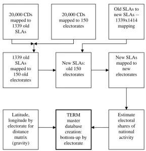
Figure 1: Devising a bottom-up database by electorate for Australia

Key: Old SLAs = statistical local areas in 2001 census; New SLAs = statistical local areas in 2006 census; CDs = voting collection districts;

Old electorates= 2004; New electorates= 2007.

Sources: ABS catalogue 1216.0, July 2006;

http://www.abc.net.au/elections/federal/2007/results/electorateindex.htm

6_{Our resulting 172 sector, 154 region master database is the largest we have devised for the TERM model, with a}

size of 667 megabytes. 20,000 CDs

mapped to 1339 old

SLAs

20,000 CDs mapped to 150

electorates

Old SLAs to new SLAs --

(11)

The choice of aggregation for our simulation depends on the focus of our study. In an election, most interest is in the marginal electorates. For example, following the 2007 election, just 46 of the 150 electorates require a swing of less than 6.0% to oust the sitting member. Only 27 seats changed parties in the 2007 election, which was notable for a large swing against the incumbent government that resulted in a change in government. Of those 27, only 8 were not predominantly urban seats. The problem with urban seats is that they tend to be relatively homogeneous,

dominated in industry structure by services sectors, with relatively small shares being

contributed by primary or secondary industries. Unless we have additional data by electorate of relevance to swinging voters, such as the ratio of household debt servicing to income, there is little to distinguish one seat from another. Consequently, a simulation based on an aggregation that represents marginal seats individually may reveal little – unless we obtain further relevant data by electorate. This is in marked contrast to several decades ago, when highly protected manufactures were often concentrated in marginal electorates. In our particular scenario, we chose to preserve electoral detail in the resource-rich regions of Western Australia, Northern Territory and non-metropolitan Queensland, while aggregating remaining electorates mostly to relatively broad regions.

The scenario: booms and busts between the elections

In our simulation, we concentrate on two economic events that have affected regional Australia between the 2004 and 2007 elections. The first is the terms-of-trade boom. Demand for raw materials by China and India has resulted in soaring commodity prices relative to those of mid-2004 (the mid-2004 election was held in October). The second is drought. In 2006, south-eastern Australia and much of the eastern seaboard to the north suffered below average rainfall. The Snowy Mountains area (the main catchment region for the southern Murray-Darling basin irrigation regions) experienced record rainfall deficiencies in 2006. The drought had a moderate impact on water allocations and output in irrigation regions in 2006, with much more severe impacts in 2007 as rainfall in catchment regions remained below average.

Droughts since the turn of the millennium have resulted in other crises. All mainland capital cities other than Darwin, plus many regional cities, have been placed on water restrictions as a combination of drought and rising populations have placed severe pressure on existing urban water resources. We do not attempt to model the economic impact of urban water restrictions in this simulation. Recurrent droughts have also fuelled severe bushfires – even in capital cities (Sydney late in 2002, with more outbreaks since and Canberra in January 2003). Community perceptions of climate change have altered in the wake of recurrent droughts over the past half a dozen years. Differences persisted in the attitudes of the main political parties to climate change, and appeared to have some impact on voting patterns at the 2007 election. Again, we have not attempted to model anything to do with drought other than the direct impact on farm output. There are a number of election issues that may have been much more significant in the final analysis than the terms-of-trade boom or drought. We have chosen these events because they translate readily to regional economic impacts.

(12)

tight labour market – national aggregate employment is fixed. At the same time, we assume that although national aggregate investment is fixed, investment by sector follows variations in rates-of-return. National aggregate household consumption is fixed, while following income earned by labour at the regional level. Fixed national consumption might be consistent with the Reserve Bank keeping a lid on excessive demand by adjusting interest rates. Similarly, we assume that aggregate government consumption is exogenous, so that windfall royalties from the terms-of-trade contribute to increases in the budget surplus.

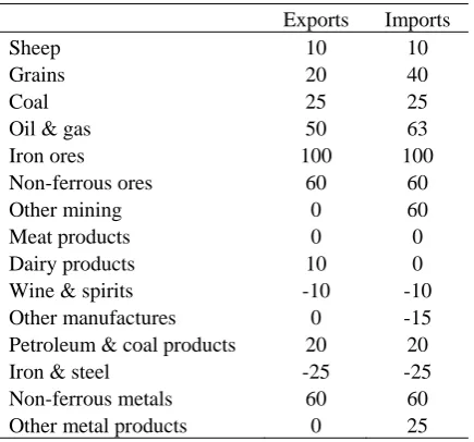
Table 1: Shocks to export and import prices

Exports Imports

Sheep 10 10

Grains 20 40

Coal 25 25

Oil & gas 50 63

Iron ores 100 100

Non-ferrous ores 60 60

Other mining 0 60

Meat products 0 0

Dairy products 10 0

Wine & spirits -10 -10

Other manufactures 0 -15

Petroleum & coal products 20 20

Iron & steel -25 -25

Non-ferrous metals 60 60

Other metal products 0 25

Source: ABARE (2007).

Table 1 shows the price shocks ascribed to selected commodities. Australia is a large exporter of gas and significant net importer of oil. Hence, the export price shock to oil and gas is smaller than the corresponding import price shock, as gas has a significant weight in exports and zero weight in imports. Some of the commodity prices are relatively moderate, as sharp price increases occurred in the months prior to the 2004 election – we have ascribed shocks to reflect price hikes from the 2004 to 2007 elections.

(13)

Table 2: Productivity level due to drought by region/electorate (100=average year)

Rural NSW 50

Regional VIC 50

Capricornia QLD 87

Groom QLD 83

Maranoa QLD 67

Flynn QLD 91

Rural SA dryland 50

Rural SA irrigated 59

Brand WA 87

Forrest WA 91

OConnor WA 71

Bass TAS 67

Braddon TAS 67

Denison TAS 67

Lyons TAS 67

Source: Authors’ estimates based on two-year rainfall deficiencies provided by the Bureau of Meteorology.

Regional outcomes

Table 3 shows macroeconomic outcomes by region. The bottom row shows national results. The real GDP loss (-0.7%) shown for the national economy is a consequence of drought.

In export-oriented sectors, the real capital rental will rise as export prices rise in the absence of any increase in capital stocks (r is the capital rental minus the GDP deflator). Usually, any increase/decrease in regional aggregate employment (indicating a decrease/increase in the K/L ratio if capital is fixed) must be accompanied by a decrease/increase in real producer wages (w, nominal wages minus the GDP deflator) relative to the rate of return on capital (r). But since capital is fixed in each industry in the short-run, and by assumption employment is fixed in national aggregate, employment at the regional level is only likely to increase if that region’s factor rental ratio w/r falls more than the national ratio. The national factor rental ratio falls by 25% (national w falls by 7.8%, national r rises by 23.0%: [100-7.8]/[100+23.0]=0.748). The electorate of Kalgoorlie in Western Australia, due to the doubling of iron ore export prices, has the largest fall in the factor rental ratio and is accompanied by the largest percentage increase in employment of all the regions. But there is not a strict ranking of employment outcomes

(14)

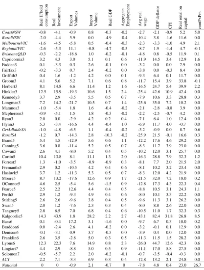
Table 3: Regional macro outcomes (% change from base case)

Real H’hold consumptio

n Real Inves tm e n t

Export Vol

u

mes

Import Vol

u me Real GDP Aggr ega te Employm e n t Avg rea l wage GDP def lat o r CP I Real r en a l on ca pi tal contPxPm

CoastNSW -0.8 -4.1 -0.9 0.8 -0.3 -0.2 -2.7 -2.1 -0.9 5.2 5.0

RuralNSW -2.0 -4.4 5.9 0.0 -4.9 -0.4 -10.4 3.8 -1.6 11.6 0.0

MelbourneVIC -1.6 -4.5 -5.8 0.5 -0.4 -0.3 -2.3 -3.3 -1.0 4.9 2.1

RegionalVIC -2.6 -5.3 11.1 -0.8 -4.7 -0.5 -8.7 1.9 -1.4 4.7 -0.1

BrisbaneQLD -0.3 -2.2 -18.6 1.0 -0.2 -0.1 -4.8 0.8 -0.5 11.9 0.1

Capricornia3 3.2 4.3 3.0 5.1 0.1 0.6 -11.9 14.5 3.4 12.9 1.6

Fadden3 0.1 -3.3 0.3 2.6 -0.1 0.0 -3.2 0.0 0.0 7.9 0.0

Fairfax3 -0.2 -3.3 0.7 2.4 -0.2 0.0 -3.8 0.0 -0.3 8.4 0.0

Griffith3 0.4 1.6 -1.2 4.2 0.0 0.1 -9.3 6.4 0.1 11.7 0.0

Groom3 4.1 5.6 5.2 7.1 0.6 0.8 -11.7 15.4 3.9 33.8 -0.1

Herbert3 8.1 14.8 6.6 11.4 1.2 1.6 -16.5 24.7 5.4 39.9 2.2

Hinkler3 12.5 15.9 -19.3 10.6 1.5 2.4 -25.4 42.6 10.9 42.4 0.0

Kennedy3 3.7 2.9 -3.5 5.5 0.5 0.7 -7.9 10.6 3.3 28.8 0.3

Longman3 7.2 14.2 -21.7 10.5 0.7 1.4 -25.6 35.0 7.2 10.2 0.0

Maranoa3 -1.0 -5.4 1.8 1.6 -0.4 -0.2 -2.1 -2.8 -0.8 3.9 0.0

Mcpherson3 -0.9 -5.1 1.5 1.8 -0.3 -0.2 -2.2 -2.5 -0.7 4.2 0.0

Ryan3 2.0 0.0 -2.9 4.2 0.2 0.4 -7.1 6.4 1.0 12.4 0.0

Flynn3 5.3 -3.4 -16.6 4.4 -0.4 1.0 -6.9 11.7 4.0 -0.7 0.0

GrtAdlaideSA -1.0 -4.8 -6.5 1.1 -0.4 -0.2 -3.2 -0.9 0.0 8.7 0.6

RuralSA -1.2 0.7 -14.3 2.8 -10.3 -0.2 -25.9 21.5 -0.1 16.6 0.3

Brand5 5.4 4.5 -12.9 5.6 0.6 1.1 -12.2 17.6 4.6 29.2 0.0

Canning5 3.6 0.8 -11.4 5.2 0.5 0.7 -8.3 11.7 3.9 23.0 0.0

Cowan5 2.6 4.1 -8.0 5.2 0.4 0.5 -10.2 12.0 3.1 25.7 0.0

Curtin5 10.4 13.8 8.1 11.1 1.3 2.0 -16.3 28.8 7.9 32.3 1.2

Forrest5 1.3 -1.0 -3.5 -0.9 -0.9 0.3 -8.1 7.7 2.0 21.5 2.0

Fremantle5 2.9 0.2 -10.5 4.2 0.4 0.6 -8.1 10.2 3.2 23.4 0.0

Hasluck5 3.7 1.2 -11.3 5.3 0.5 0.7 -8.3 12.0 4.2 21.9 0.0

Moore5 8.7 13.2 -17.6 12.6 0.9 1.7 -21.5 32.0 7.2 18.0 0.2

OConnor5 4.6 2.5 -5.4 5.6 -1.5 0.9 -12.8 17.3 4.3 22.3 0.4

Pearce5 2.5 2.2 12.6 4.4 0.4 0.5 -8.8 10.5 3.1 24.3 1.1

Perth5 2.9 1.2 -9.3 4.9 0.4 0.6 -8.0 10.1 3.3 22.2 0.0

Stirling5 2.6 2.6 -9.6 3.8 0.4 0.5 -9.6 11.3 3.1 26.2 0.0

Swan5 2.0 1.2 -7.6 2.3 0.3 0.4 -8.0 8.8 2.6 22.0 0.0

Tangney5 2.8 6.5 7.0 6.8 0.4 0.6 -10.5 11.0 1.7 32.3 0.3

Kalgoorlie5 14.3 43.9 1.8 28.2 2.2 2.7 -43.1 82.4 31.8 26.8 8.5

Bass6 0.1 -0.4 17.2 3.1 -1.6 0.0 -9.7 6.7 0.3 18.0 0.2

Braddon6 0.0 -2.4 2.6 4.1 -0.2 0.0 -3.2 -0.1 0.1 12.9 0.0

Denison6 -0.1 -3.1 0.9 3.7 -0.5 0.0 -3.9 0.4 0.0 12.0 0.0

Franklin6 2.6 3.5 -2.8 5.0 0.3 0.5 -11.3 11.5 1.5 28.2 0.0

Lyons6 12.3 22.3 7.6 14.9 0.8 2.3 -26.0 44.7 12.6 42.3 0.6

Lingiari7 4.4 2.9 -8.8 5.0 0.5 0.9 -11.1 17.0 5.8 27.5 0.0

Solomon7 -0.5 -5.7 2.2 2.0 -0.2 -0.1 -0.7 -3.5 -0.4 -0.3 0.0

ACT 2.2 7.1 -3.3 6.9 0.3 0.4 -12.8 13.2 2.1 24.8 0.0

National 0 0 -0.9 2.1 -0.7 0 -7.8 4.8 0.4 23.0 26.7

(15)

terms-of-trade increase. Yet there is not a close correlation between the employment results and the terms-of-trade contribution result. Coastal New South Wales makes the second largest contribution to the terms-of-trade gain due to a rise in coal export prices and the massive coal export base in the region. In the choice of aggregation, the Hunter electorate was combined with other coastal electorates in New South Wales. Had Hunter been represented separately, the employment increase may have been of a similar percentage to that for Kalgoorlie. Employment tends to move from non-mining to mining sectors in the scenario. That there is an employment loss simulated for Coastal NSW reflects the dominance of non-mining activity in the region, despite the exports of coal from the Hunter Valley. The contribution of the Hunter electorate is masked by the aggregation: it accounts for most of the terms-of-trade contribution in the final column, but its positive employment impact is more than offset by job losses elsewhere in the composite region.

Since national aggregate consumption is exogenous by assumption, we can expect regions to increase or decrease their share of national GDP according to relative regional outcomes. Nominal household consumption in each region is tied to nominal labour earnings. Aggregate consumption by region increases/decrease as regional employment increases/decreases. Aggregate consumption follows in GDP in showing marked disparities between regions.

The impact on relative prices across regions

In response to a large terms-of-trade impact and drought, prices will play a significant

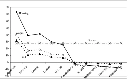
adjustment role in the short run. The most volatile short-run price in the model will be the price of housing. This is because housing consists almost entirely of capital, which is fixed by assumption in the short run. Also, housing is income elastic. This implies that when income grows, and the stock of housing is fixed, there will be large increase in the housing price. The 10 regions shown in figure 1 include the five with the largest percentage increase in the price of housing. The figure also includes the five regions with the largest decrease in the housing price. The percentage change in housing price is generally much larger than the percentage change in regional aggregate consumption in this short-run setting.

Kalgoorlie has the largest percentage increase in the price of housing – had we represented the Pilbara region separately in the simulation, its housing price increase would have been even larger again, due to the concentration of the iron ore export price increase in the region (figure 2).7 The CPI in each region includes a substantial house price weighting. For example, in

Kalgoorlie, the contribution of housing is 27.4% out of a total CPI increase of 31.8% (i.e., seven-eighths of the total). Non-housing price hikes have been moderated in most regions particularly by the falling price of imported other manufactures (see table 1).

7_{When we repeat the simulation with the DeGrey statistical subdivision (which includes Port Hedland and part of}

(16)

Figure 2: Prices at the regional level (% change relative to nominal exchange rate) -20 -10 0 10 20 30 40 50 60 70 80 Kal goo rlie5 Hink ler3 Lyons 6 Cur tin5 Mo ore5 GrtAd laid eSA Rura lSA Mel bou rneV IC Rura lNS W Regi onal VIC Housing Shares CPI Wages

There are two reasons why the short-run closure prevents a larger non-housing impact occurring for consumer goods and services. First, national aggregate consumption is exogenous and unchanged, thereby limiting the impact of the terms-of-trade boom on relatively income-elastic service sectors. Second, we assume that the drought does not affect national employment. Instead, jobs lost in the farm sector are able to move into mining, taking heat out of the labour market. In addition, we have not attempted to model different demand increases for different labour skills. In reality, it might be that at the same time as the drought has provided additional workers for the mining sector, there may also have been a larger increase in demand for

relatively skilled labour than unskilled labour. Such a bias may have inflationary consequences. Figure 2 provides some insights into who have been the biggest winners and potentially the biggest losers from the terms-of-trade boom. House owners in mining regions have done well from the boom. Those seeking to rent a house in mining regions would have found that much of the additional salary that attracted them to the mines has gone in housing. Consequently, we have assumed that the labour response to regional wage differentials is relatively small. In addition, mining operations tend to be located in remote regions, so that large wage premiums are necessary to attract workers. The rise in nominal wages exceeds CPI only marginally in mining regions due to housing costs, even with relatively inelastic inter-regional migration.

(17)

shareholders throughout the nation have experienced the same windfall gain due to the terms-of-trade boom.

The biggest losers in this scenario have been farmers directly affected by drought. Consequently, Rural South Australia, Rural New South Wales and Regional Victoria are three of the four regions that lose most. However, a return to better seasons is likely to be accompanied by relatively high farm output prices. It is possible therefore that fortunes on the land could turn around relatively quickly.

Other losers are those without substantial equity in their place of residence. Rising house rentals and rising interest rates (to keep inflation within limits prescribed by the Reserve Bank) may make some households worse off. Since the Commonwealth and state governments have collected windfall royalties and revenues from the boom, there has been some opportunity for spreading gains across regions. However, fiscal responses have been tempered by a concern that monetary responses alone will be insufficient to keep inflation in check. Outside of mining regions, the spread of rising house prices may not have been accompanied by rising incomes. We discuss why house prices might rise outside mining regions under the heading.

The impact of mining booms on regional house prices

It would appear that housing prices in non-booming regions fall relative to the nominal exchange rate. This is potentially misleading, as there has been a substantial nominal appreciation with the onset of the terms-of-trade boom. Moreover, many mining employees work on a fly-in, fly-out basis. Increased incomes may end up being spent in capital cities. Perth was the first capital to experience booming real estate prices – median prices rose by almost 40% in 2006 (Real Estate Institute of Australia, 2008). The Real Estate Institute did not anticipate the large increase in house prices in Melbourne in 2007. We might attribute the increase to rising purchases in the Melbourne market from cashed-up winners in the mining industry.

The terms-of-trade boom in Australia has brought with it accelerated investment in the mining industry. This in turn has led to huge jumps in house prices in some mining regions. For example, in Port Hedland, the median house price in the twelve months to February 2008 was almost $700,000. 8 With a booming local economy, Port Hedland’s housing needs reached a crisis point in 2007. Usually, income-elastic service sectors do well during such boom. But some service industries in Port Hedland have been caught in a cost squeeze: available labour has been too scarce for them to continue operating and their own housing costs have risen beyond

affordability.9

Construction phases in mining towns tend to result in a boom-bust cycle in local housing prices. In the case of a construction phase with a known timetable, the rationality of price increases in questionable. Supposing rents in a town double during a construction phase, as we modeled for the Port Hedland region with a finer regional disaggregation (see footnote 2). The price of housing stock should only increase sufficiently to cover the temporary rental hike, plus reflect

8_{http://www.domain.com.au/Public/suburbprofile.aspx?mode=research&searchTerm=Port%20Hedland#mapanchor} 9_{Radio National based a story on Port Hedland’s housing crisis in December 2007:}

(18)

some expectation of longer term increases in regional income. Using a discounted income stream calculation, a four year construction phase might increase the stock price by around 30%.

Housing busts are likely to follow when percentage stock price increases approach the

percentage increase in rental rates. There may be specific reasons why house prices in one town are high. The perception in Port Hedland might be that the mining boom will last indefinitely. Even if this is so, mining itself is not labour-intensive, whereas construction is – which implies that demand for housing will decline at the end of the construction phase. The need for dwellings to be cyclone-proof in the region, its extreme isolation and its extremely hot climate may each have slowed the housing supply response to escalating prices.

Summary of findings from an electoral representation

Previous applications of TERM have shown dispersions between winners and losers by regions or, in the case of drought, a concentration of losers in predominantly agricultural regions. A representation by electorates may make regions more homogeneous than a representation by statistical regions. Some of the insights from TERM simulations in the past have come from capturing the differences between regions in industry composition. At present, marginal seats are concentrated in outer suburban regions with relatively homogenous industry composition.

Most of the insights gained in this study would have been apparent in the usual regional representation of TERM (i.e., based on ABS statistical divisions). The same terms-of-trade and droughts shocks applied to such a representation would have revealed winners among major mining regions, losers in agriculture and losers in urban areas in non-mining states, at least in the short run.

Perhaps the greatest weakness of all in an electoral representation within a multi-regional CGE model is that although voters’ perceptions of economic issues influence elections, other issues may play a much bigger role in a particular election. It would appear that the change of government in Australia’s 2007 election arose mainly from non-economic issues.

5. Conclusions

The demand for and use of massive master databases in multi-regional CGE models is likely to grow. Regional economies play some part in politics. A recurrent danger in policy formulation is that regional considerations will confound policy objectives. Policy-makers justify some policies that may not appear to be economically justifiable on the grounds that they will strengthen regional economies. For example, in irrigation regions of Australia, there are some fears that permanent water trades and diversions of water to the environment will weaken regional economies. Authorities have used these concerns to constrain permanent water trades. Yet the data we have gathered in the process of enhancing our capability to model regional economies point to the increasing roles of health care, education and aged care even in ostensibly

(19)

reduce Australia’s greenhouse gas emissions. In previous decades, successive federal governments slowed tariff reductions in response to regional considerations.

Once we had gathered data for over 1400 SLA regions, we were in a position to generate a master regional database of dimensions beyond relatively standard computing power. Rather than constrain ourselves to a smaller master database within the computing capabilities that did not fully utilize available data, we chose the variable disaggregation approach to generate a number of different master regional databases.

Within the GTAP community, the emphasis in global modeling appears to be switching increasingly from trade reform scenarios to environmental scenarios. This is likely to result in growing demand for databases with more sectoral detail. Then, sectors might be split so as to capture different greenhouse gas emissions per unit of energy from different fuel types within the industry structure of the database. To the extent that different modes of transport use different energy sources, disaggregation of transport might also provide advantages when it comes to environmental scenarios. Similarly, as water scarcity becomes a global issue, a more

disaggregated representation of agricultural sectors will assist water-related modeling.

This paper has introduced a bottom-up representation of the Federal electorates of Australia to a multi-regional CGE model, TERM – perhaps the most ambitious regional representation we have undertaken. Although this sounds like a politically attractive idea, at present the electorate-based model has little advantage over previous representations of TERM.

There may be some advantages from extending the number of regions in the master TERM databases we have developed for other countries. For example, available data in China reveal marked disparities between household expenditures between urban and rural regions in each province. We have a developed a TERM-based model of China covering all 31 provinces and municipalities (Horridge and Wittwer, 2007). In the future, it might become possible to split each province or municipality into urban and rural components, increasing the number of regions in the Chinese database to around 60. Some of the methods we have developed in the creation of a variable disaggregation TERM database of Australia might assist us in preparing an enhanced database of China.

References

ABARE (2007), Australian commodity statistics.

Adams, P., Horridge, M. and Parmenter, B. (2000), MMRF-Green A dynamic, multi-sectoral, multi-regional model of Australia, Centre of Policy Studies working paper OP-94.

(20)

Horridge, M., Madden, J. and Wittwer, G. (2005), “Using a highly disaggregated multi-regional single-country model to analyse the impacts of the 2002-03 drought on Australia”, Journal of Policy Modelling, 27(3): 285-308.

Horridge, M. and Wittwer, G. (2007), “The economic impacts of a construction project, using SinoTERM, a multi-regional CGE model of China”, Centre of Policy Studies Working Paper G-164, June.

Real Estate Institute of Australia (2008 and previous years), Real Estate Market Outlook,

www.reiaustralia.com.au/documents/2008_REAL_ESTATE_MARKET_OUTLOOK.doc;