Menzies Building
Monash University Wellington Road
CLAYTON Vic 3168 AUSTRALIA
Telephone:
from overseas:
(03) 905 2398, (03) 905 5112
61 3 905 2398 or 61 3 905 5112
Fax numbers:
from overseas:
(03) 905 2426, (03)905 5486
61 3 905 2426 or 61 3 905 5486
[email protected]
Computing Solutions for Large
General Equilibrium Models Using
GEMPACK
by
W.Jill Harrison and K.R. Pearson
Impact Project
Monash University
Preliminary Working Paper No. IP-64 June 1994
ISSN 1031 9034
ISBN 0 7326 0716 7
C
ENTRE
of
P
OLICY
S
TUDIES
and
the
I
MPACT
i
GEMPACK is a suite of general-purpose economic modelling software especially suitable for general and partial equilibrium models. It can handle a wide range of economic behaviour and also contains a versatile method for solving intertemporal models. GEMPACK provides software for calculating accurate solutions of an economic model, starting from an algebraic representation of the equations of the model. These equations can be written as levels equations, linearized equations or a mixture of these two. The software provides a range of utility programs for handling the economic data base and the results of simulations, and is fully documented from a user's point of view.
GEMPACK is used to implement and solve a number of economic models including several single-country models (of which the ORANI model of Australia is perhaps the best known), multi-country trade models, regional models and intertemporal (or dynamic) models. GEMPACK runs on a wide variety of computers including 80386/80486 microcomputers running DOS, Windows or OS/2, Apple Macintosh computers, Unix machines, DEC VAX and Alpha machines running VMS.
This paper gives an overview of the current release of GEMPACK (Release 5.1, April 1994). Included are descriptions of
• the algebra-like language used to describe and document the equations of an economic model,
• the operation of the pre-processor TABLO which converts the equations of the model to a form suitable for computing solutions of the model,
• the solution methods used for producing accurate solutions of the model,
• the facilities for specifying and carrying out simulations, including the options for varying the choice of endogenous and exogenous variables and the variables shocked,
• the condensation facility which makes it possible to solve very large models,
• the utility programs for assisting in managing the data bases on which models are based,
ii
page
Abstract i
1 INTRODUCTION 1
1.1 Development of GEMPACK 1 1.2 Software For Equilibrium Models 2 1.3 Overview Of The Paper 3
1.4 Simulations 4
2 IMPLEMENTING MODELS 6
2.1 Writing Down The Equations Of A Model 6 2.1.1 The Equations of Stylized Johansen 8 2.2 Data Requirements For A Model 9 2.2.1 The Data Requirements For Stylized Johansen 10 2.3 Constructing The TABLO Input File For A Model 10 2.3.1 The TABLO Input File For Stylized Johansen 11 2.4 Linearized Representations And Update Statements 13 2.5 Different Representations (Levels, Linearized or Mixed) 15 2.5.1 TABLO Linearizes Levels Equations 16
2.6 Example Models 16
3 CARRYING OUT SIMULATIONS 17 3.1 Interpreting The Results of A Simulation 17 3.1.1 A Simulation With Stylized Johansen 17 3.2 Specifying A Simulation 19 3.2.1 An Example Command File 20 3.3 Steps In Carrying Out A Simulation 22 3.4 Different Closures And Shocks 24 3.4.1 Different Closures 25
3.4.2 Shocks 26
iii
6.1 Data Preparation 35
6.2 Result Processing And Reporting 36
7 INTERTEMPORAL MODELS 36
8 COMMUNICATING MODELS TO OTHERS 37
9 SOFTWARE ASPECTS 37
9.1 Standard Program Options 37
9.2 Subroutines 38
9.3 Model Size And Program Parameters 38
9.4 History Of Files 39
9.5 Binary Files 39
9.6 No Special Windows Features 39 9.7 Solving Sparse Systems Of Linear Equations 40 9.8 Compilers On 386/486 PCs And Macintosh PCs 40 10 CHANGES IN COMPUTING ENVIRONMENT 40 11 DIFFERENT VERSIONS OF GEMPACK
11.1 Source-code Versions 41 11.2 Executable Image Version 41 11.3 Demonstration Version 41 11.4 Current GEMPACK User Documentation 42 APPENDIX A THE TABLO INPUT FILE FOR THE STYLIZED
JOHANSEN MODEL 42
APPENDIX B INITIAL VALUE PROBLEMS 47 B.1 Simulation Problems - A Definition 48 B.2 Converting a Simulation Problem To
An Initial Value Problem 49 B.3 Setting up the Initial Value Problem 52
iv
Table 2.1.1a Levels And Linearized Equations of the Stylized
Johansen Model 7
Table 2.1.1b Levels Variables for Stylized Johansen 8 Table 2.1.1c Parameters for Stylized Johansen 9 Table 2.1.1d Equations for Stylized Johansen 9 Table 3.1.1a Input-output Data Base for Stylized Johansen 18 Table 3.1.1b Part of Simulation Results File 18 Table 4.3 Multistep and Extrapolated Results 29 Table 4.4 Individual Column Results for Johansen Simulations 31
LIST OF FIGURES
U
SING
GEMPACK
by
W. Jill HARRISON and K.R. PEARSON
1 INTRODUCTION
GEMPACK is a suite of general-purpose economic modelling software especially suitable for general and partial equilibrium models. It can handle a wide range of economic behaviour and also contains a versatile method for solving intertemporal models.
GEMPACK software is being used in over 50 organizations around the world (universities, government departments and private sector firms). It is used to implement and solve a number of economic models including several single-country models (of which the ORANI model of Australia is perhaps the best known), multi-country trade models, regional models and intertemporal (or dynamic) models.
GEMPACK provides software for calculating accurate solutions of an economic model, starting from an algebraic representation of the equations of the model. These equations can be written as levels equations, linearized equations or a mixture of these two.
The software provides a range of utility programs for handling the economic data base and the results of simulations, and is fully documented from a user's point of view.
GEMPACK runs on a wide variety of computers including
• 80386/80486 microcomputers running DOS, Windows or OS/2,
• Apple Macintosh computers,
• Unix machines,
• DEC VAX and Alpha machines running VMS, and
• other mainframe, mini and microcomputers with an ANSI standard Fortran 77 compiler.
1.1 Development Of GEMPACK
The aim in developing GEMPACK has been to provide a suite of tools (or, expressed more exotically, a modelling environment) for equilibrium modellers which will free them from most computing-related difficulties and constraints, and will allow them to concentrate on the economic aspects of their models. In particular, modellers using GEMPACK should never have to write their own programs either to solve their model or to communicate it (theory or data) to the computer or to other modellers. The algebraic representation of models used in GEMPACK (see section 2 for more details) has been chosen and designed with the intention that
(b) it should be an intelligible, essentially self-contained, documentation of the model, and
(c) it should be the means of communicating the model to others who wish to understand, use and/or modify the model.
An important part of this was the desire to provide a tool that would reduce by an order of magnitude the research resources (especially person-months) required to build and maintain a new model. It has been estimated that, compared to the situation which was common in the middle 80s when modellers often wrote their own programs (for example, in Fortran), the use of GEMPACK reduces this research input by over 85% - see Powell (1988).
The rationale behind the development of GEMPACK is still essentially as set out in Pearson (1988). An introduction to the algebraic language used by GEMPACK can be found in Codsi and Pearson(1988); however that paper was written before GEMPACK was able to produce accurate solutions of the (usually nonlinear) equations of a model, and before GEMPACK allowed explicit levels equations. An introduction to the intertemporal capabilities of GEMPACK can be found in Codsi, Pearson and Wilcoxen (1992).
The software is general-purpose in the sense that it can be used to model a wide range of economic behaviour. It imposes no fixed recipe of possible behaviours; rather it allows most sorts of behaviour that can be expressed as algebraic equations. The software "knows" no economics; it is the modeller’s responsibility to ensure that the algebraic equations are accurate. The algebraic language does not allow explicit inequalities in the system solved. However, because linearized equations are allowed, various sorts of optimising behaviour whose explicit solution in the levels may be complicated or not known analytically can be handled; the first-order conditions can be used instead of the optimising form of the problem.
1.2 Software for Equilibrium Models
There are various general-purpose software packages available for solving equilibrium models. Probably the best known is the fine GAMS software (see Brooke el al (1988)), which now incorporates MPS/GE (see Rutherford (1989)). There is a large overlap in the sorts of models that can be handled by GAMS, MPS/GE and GEMPACK. There are many similarities between these. For example, the algebraic languages used by GAMS and GEMPACK are similar; the development of this interface for GEMPACK benefited from our knowledge of the GAMS language. There are also significant differences between these packages. A recent review of some software for equilibrium modelling (including GEMPACK and MPS/GE, but not GAMS) can be found in Harrigan (1993).
It is not our intention here to compare GEMPACK with other packages (we leave this to others), but rather to give an up-to-date description of the main features of GEMPACK (as in Release 5.1). We believe that the existence of overlapping but different general-purpose tools for GE modelling has proved, and will continue to prove, a stimulus for such modelling. Modellers are free to choose the tool which is best suited to the task before them, or with which they are most familiar.
model. Hertel et al. (1992) address this issue and explain that, despite the linear representation often used to communicate models to GEMPACK, GEMPACK can produce the same accurate solutions of the underlying levels equations of the model as are produced by systems such as GAMS which usually begin from explicit levels equations. More details can be found in section 4 below.
Features of GEMPACK which, so far as we are aware, are not explicitly available in any other software are
• automatic algebraic condensation of a model (see section 5). (This makes it possible to solve much larger models than would otherwise be feasible.)
• the acceptance of wholly linearized equations or a mixture of levels and linearized equations. (See Harrison et al. (1993) and section 2 below for more details.)
• software for computing several Johansen solutions simultaneously (see section 4.4).
1.3 Overview Of The Paper
This paper gives an overview of the current release of GEMPACK (Release 5.1, April 1994).
The algebra-like language used to describe and document the equations of an economic model is described in sections 2.1 and 2.3. The pre-processor program TABLO converts the equations of the model to a form suitable for carrying out simulations and computing solutions of the model. The equations, which can be (non-linear) levels equations or linearized equations or a mixture of the two, are always converted to a linearized representation of the model; any levels equations are symbolically differentiated by the software (see sections 2.4 to 2.7).
In section 3, we describe the facilities for specifying and carrying out simulations, including the options for varying the choice of endogenous and exogenous variables and the variables shocked. These include GEMPACK Command files which consist of a number of self-documenting statements such as
exogenous to txs tms tm tx qo(ENDW_COMM,REG) ; rest endogenous ;
shock tms("food","USA","EEC") = -10.0 ;
The solution methods used for producing accurate solutions of the model are given in section 4. These multi-step methods, which are based on the linearized representation produced by TABLO, are variants of well-known numerical methods for solving initial-value problems involving differential equations.
The condensation facility in GEMPACK, which makes it possible to solve very large models, is described in section 5. The software can be directed to make algebraic substitutions symbolically in the system of linearized equations to reduce the system actually solved to a manageable size. The values of those variables which are substituted out are available, if desired.
(including those with different operating systems). The GEMPACK system of communicating models to other modellers (and other machines) is described in section 8.
A brief introduction to the method GEMPACK uses for solving intertemporal models is given in section 7. In section 9, we describe various aspects of the software design. Changes in the computing environment, discussed in section 10, have caused a move to the use of PCs instead of mainframes for many users.
Finally, details are given in section 11 of the different versions of GEMPACK. Most are source-code versions, which require a suitable Fortran compiler; for these the size of models that can be handled is limited only by the amount of memory available. Others are executable-image versions, which can only handle models of limited size. There is a Demonstration Version available essentially free for use in teaching or for modellers wanting to find out more about how the software works.
1.4 Simulations
"Simulation" can mean different things in different contexts. Here we describe what it typically means in a general equilibrium model setting.
Solving models within GEMPACK is always done in the context of a simulation. The values of certain of the variables, the exogenous variables, are specified and the software calculates the values of the remaining ones, the endogenous variables. The new values of the exogenous variables are usually given by specifying the percentage changes (increases or decreases) from their values in the original (pre-simulation) solution. Similarly the results of the simulation, the endogenous variables, are usually reported as percentage changes.
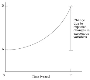
General equilibrium models were first used to give policy advice. More recently, some have been used for forecasting. Below we follow Horridge et al.
(1993) in giving a brief explanation of these.
Change due to Tariff
Employment without Tariff Employment
Figure 1.4a: Comparative-Static Interpretation of Results
0 T
A B C
Employment with Tariff
Time (years)
Employment
Change due to expected changes in exogenous variables D
A
0 Time (years) T
For forecasting, it is necessary to feed in (as shocks to the model) expected changes in all exogenous variables over the time span of the simulation; the model should then report changes in the endogenous variables. In Figure 1.4b, the initial (pre-simulation) solution and data base are thought of as representing the economy now, and the final (post-simulation) solution and data base as those that will be in 5 years' time. The results reported by GEMPACK are percentage changes over the period. For example, if employment is A now and will be D in 5 years' time (given the expected changes in the exogenous variables), the result reported will be the percentage change 100(D-A)/A from A to D.
Typically only a small number of exogenous variables are shocked in policy-advice simulations but a large number are shocked in forecasting simulations. We look at simulations in greater detail in section 3.
2
IMPLEMENTING MODELS
A model is implemented in GEMPACK when
(1) the equations describing its economic behaviour are written down in an algebraic form,
(2) data describing one solution of the model are assembled, to be used as a starting point for simulations, and
(3) a text file, containing the equations (written in an algebra-like syntax) and information about the data, is prepared. This file is called a TABLO Input file since TABLO is the name of the GEMPACK program which processes this file and converts the information on it to a form suitable for running simulations on the model.
These three stages are described in sections 2.1 to 2.3 respectively. We illustrate the process by showing, in sections 2.1.1, 2.2.1 and 2.3.1, how these stages are carried out for the Stylized Johansen model. This small model, which is used for teaching purposes, is described in Chapter 3 of Dixon et al. (1992).
In sections 2.4 and 2.5 we discuss briefly the differences between linearized, levels and mixed representations of a model. Section 2.6 contains references to models implemented via GEMPACK and those usually supplied with GEMPACK.
2.1 Writing Down The Equations Of A Model
TABLO Input files contain the equations of a model written down in a syntax which is very similar to ordinary algebra. Once the equations of the model are written down in ordinary algebra, it is a simple matter to put them into a TABLO Input file.
Levels or linearized versions of the equations can be used, or a mixture of these two types. For example, if a certain dollar value D is the product of the price P and quantity Q, the levels equation is
D = PQ
and the associated linearized equation is
Table 2.1.1a: Levels and Linearized Equations of the Stylized Johansen Model*
Levels Form Linearized Form
consumer demands
Xi0 = αi0Y/Pi xi0 = y – pi i = 1,2
intermediate demands
Xij = αijXj
Π
t=1Pαtj t
Π
t=1(αtj)–αtj
/
[
Aj Pi]
xij = xj –(pi –
Σ
t=1 4
αtj pt )i=1, ..., 4
j = 1, 2
price formation
Pj =
Π
t=1 4(αtj)–αtj
Π
t=1 4
Pαtj
t
/
A jpj =
Σ
t=1 4
αtj pt j = 1,2
commodity market clearing
Σ
j=0 2
Xij = Xi xi =
Σ
j=0 2
[
XijXi
]
xij i = 1,2aggregate primary factor usage
Σ
j=1 2
Xij = Xi xi =
Σ
j=1 2
[
XijXi
]
xij i = 3,4numeraire
P1 = 1 p1 = 0
intermediate demands – dollar values
D ij = Pi X ij
d
ij = pi + x ij i =1, ..., 4
j = 1, 2
consumer demands – dollar values
D i0 = Pi Xi0 d i0 = pi + x
i0 i = 1, 2 * Upper-case Roman letters represent the levels of the variables; lower-case Roman letters are the
corresponding percentage changes (which are the variables of the linearized version shown in the second column). The letters P, X and D denote prices, quantities and dollar values respectively, while the symbols A and α denote parameters. Subscripts 1 and 2 refer to the (single) commodities produced by industries 1 and 2 (subscript i), or to the industries themselves (subscript j); i = 3 refers to labour while i = 4 refers to the model's one (mobile-between-industries) type of capital; subscript j = 0 identifies consumption.
2.1.1 The Equations Of Stylized Johansen
We start from the equations as written down in Chapter 3 of Dixon, Parmenter, Powell and Wilcoxen (1992), which we abbreviate to DPPW. This contains a description of the Stylized Johansen model and the derivation of these equations.
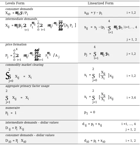
The equations of the model are shown in Table 2.1.1a. In that table, both the levels and linearized versions of each equation are shown, taken essentially unchanged from DPPW.1 Notice that, in Table 2.1a, upper case letters (for
example, X) denote levels quantities while lower case letters (for example, x) denote percentage change in the corresponding levels quantity. For our implementation of Stylized Johansen we have chosen a mixed representation, based on the shaded blocks in Table 2.1.1a. That is, we decided to use the levels versions of some of the equations (most are accounting identities and one is the numeraire equation) and the linearized versions of the top three equations (which are behavioural equations).
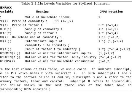
The notation in DPPW involves a liberal use of subscripts which are not suitable for the linear type of input usually required by computers (and required in the TABLO Input file). Hence we use a different notation from DPPW. The levels variables of the model are given in Table 2.1.1b.
Table 2.1.1b: Levels Variables for Stylized Johansen
GEMPACK
variable Meaning DPPW Notation
Y Value of household income Y PC(i) Price of commodity i P:i (i=1,2)
PF(f) Price of factor f P:f (f=3,4) XCOM(i) Supply of commodity i X:i (i=1,2) XFAC(f) Supply of factor f X:f (f=3,4) XH(i) Household use of commodity i X:i0 (i=1,2) XC(i,j) Intermediate input of X:ij (i,j=1,2)
commodity i to industry j
XF(f,j) Input of factor f to industry j X:fj (f=3,4;j=1,2) DVCOMIN(i,j) Dollar values for intermediate inputs (i,j=1,2)
DVFACIN(f,j) Dollar values for factor use by industry (f=3,4;j=1,2) DVHOUS(i) Dollar values for household consumption (i=1,2)
In the last column of this table, we use a colon : to indicate subscript, as in P:i which means P with subscript i. In DPPW subscripts 1 and 2 refer to the sectors called s1 and s2, subscripts 3 and 4 refer to the primary factors, labor and capital. Subscript 0 refers to households. (The dollar values in the last three rows of the table have no corresponding DPPW notation.)
Table 2.1.1c: Parameters for Stylized Johansen
Parameters Meaning DPPW Notation
ALPHACOM(i,j) Commodity exponents in production ALPHA:ij (i,j=1,2) function for sector j (E3.1.4)
ALPHAFAC(i,j) Factor exponents in production ALPHA:fj(f=3,4; j=1,2) function for sector j (E3.1.4)
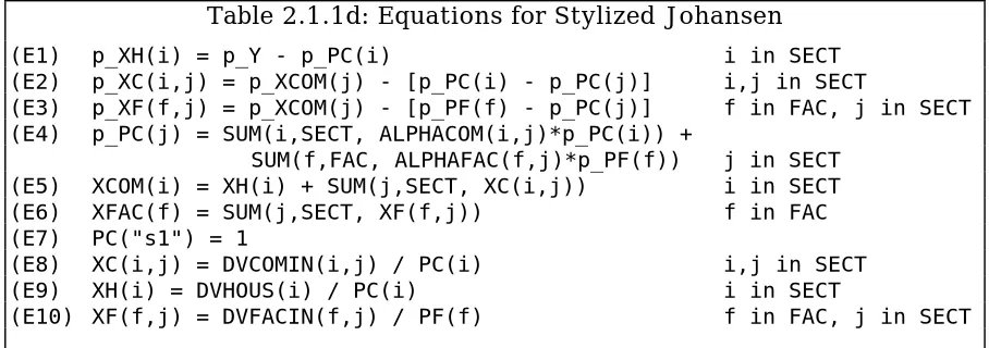
In formulating the equations (see Table 2.1.1d), it is convenient to introduce two sets SECT and FAC. SECT is the set of sectors and FAC is the set of the two factors “labor” and “capital”. Note that, since each industry produces a single commodity in this model, the set SECT doubles as the set of commodities and the set of industries (and we can use the terms sector, industry and commodity somewhat interchangeably).
Table 2.1.1d shows the selected equations from Table 2.1.1a, this time using the GEMPACK variables and notation as in Tables 2.1.1b and 2.1.1c. Note that we also use the GEMPACK convention that "p_” indicates percentage change in the relevant levels variable; for example, p_XH(i) denotes the percentage change in XH(i), household consumption of commodity i. In these equations we use "*" to denote multiplication and "/" to denote division. We also use
SUM(i, <set>, <expression>)
to denote sums (usually expressed via greek sigma) over all i in the set <set>; here <set> is SECT or FAC. The equations in the TABLO Input file (see section 2.3.1) are taken directly from Table 2.1.1d.
Table 2.1.1d: Equations for Stylized Johansen
(E1) p_XH(i) = p_Y - p_PC(i) i in SECT (E2) p_XC(i,j) = p_XCOM(j) - [p_PC(i) - p_PC(j)] i,j in SECT
(E3) p_XF(f,j) = p_XCOM(j) - [p_PF(f) - p_PC(j)] f in FAC, j in SECT (E4) p_PC(j) = SUM(i,SECT, ALPHACOM(i,j)*p_PC(i)) +
SUM(f,FAC, ALPHAFAC(f,j)*p_PF(f)) j in SECT (E5) XCOM(i) = XH(i) + SUM(j,SECT, XC(i,j)) i in SECT (E6) XFAC(f) = SUM(j,SECT, XF(f,j)) f in FAC (E7) PC("s1") = 1
(E8) XC(i,j) = DVCOMIN(i,j) / PC(i) i,j in SECT (E9) XH(i) = DVHOUS(i) / PC(i) i in SECT
(E10) XF(f,j) = DVFACIN(f,j) / PF(f) f in FAC, j in SECT
2.2 Data Requirements For A Model
As a general rule, GEMPACK requires an initial levels solution of the model. Thus it is necessary to provide data from which initial (that is, pre-simulation) values of all levels variables and the values of all parameters of the model can be inferred.
As we shall see for Stylized Johansen, and this is typical of other models, the data required are
• mainly dollar values (rather than separate prices and quantities), and
Once dollar values are known, it is often possible to set basic prices equal to 1 (this amounts to a choice of units for the related quantities), from which the quantities can be derived by dividing the dollar value by the price. [The choice of 1 for the basic price is, of course, arbitrary. Any other fixed value would be as good.]
2.2.1 The Data Requirements For Stylized Johansen
Suppose that we know the following pre-simulation dollar values:
DVCOMIN(i,j) Intermediate inputs DVHOUS(i) Household consumption DVFACIN(f,j) Factor use by industry
Then, if we set al.l the prices
PC(i) Price of commodities PF(f) Price of factors
we can infer all other levels variables in Table 2.1.1b as follows.
XC(i,j) = DVCOMIN(i,j)/PC(i) Intermediate inputs XH(i) = DVHOUS(i)/PC(i) Household use
XF(f,j) = DVFACIN(i,j)/PF(f) Factor use
Y = SUM(i, SECT, DVHOUS(i)) Household expenditure
The only other quantities in the equations (E1)-(E10) in Table 2.1.1d are the parameters ALPHACOM(i,j) and ALPHAFAC(f,j) in (E4). Because there is a Cobb-Douglas production function involved, it is well-known that these are cost shares, namely
ALPHACOM(i,j) = DVCOMIN(i,j)/DVCOSTS(j), ALPHAFAC(f,j) = DVFACIN(f,j)/DVCOSTS(j),
where DVCOSTS(j) is an abbreviation for the total costs in industry j,
SUM(i,SECT,DVCOMIN(i,j)) + SUM(f,FAC,DVFACIN(f,j)).
Thus the only data requirements are the dollar values
DVHOUS(i), DVCOMIN(i,j) and DVFACIN(f,j).
In the TABLO Input file, the pre-simulation values of these data will be read and the values of all others will be calculated from them.
2.3 Constructing The TABLO Input File For A Model
The main part of a TABLO Input file is the equations, which usually come at the end of the file. Before them must come
• the VARIABLEs (levels or linearized) occurring in the EQUATIONs;
• the SETs used to describe the different arguments of variables;
• a description of the data to be read;
• means of calculating pre-simulation values of any levels variables not read in as data (calculations are done via FORMULAs);
• means of calculating (via FORMULAs) any parameters whose values are not read in;
• the headers on the data file(s) where the different pieces of data are to be found (if the data files are GEMPACK Header Array files).
The order of these in the TABLO Input file is somewhat flexible but follows the general rule that items cannot be used until they have been declared. Thus the SET statements usually come first. Then the declarations of data files (via FILE statements) often come next, followed by the declarations of the VARIABLEs and parameters.
These ideas are best understood by example. Hence we launch straight into the preparation of the TABLO Input file for Stylized Johansen.
2.3.1 The TABLO Input File For Stylized Johansen
In this subsection we consider just two equations of Stylized Johansen, namely (E9) and (E4) in section 2.1.1 above. We show how these are written in the TABLO Input file. (We show the full TABLO Input file in Appendix A.)
Consider first the very simple equation (E9) relating prices, quantities and dollar values of household consumption. In the TABLO Input file this equation is written as2
EQUATION House # Household demand for commodity i # (all,i,SECT) XH(i) = DVHOUS(i) / PC(i) ;
where
• EQUATION is a keyword indicating that what follows is an equation,
• House is the name by which this equation is known in the model,
• the words between the hashes # form optional additional labelling information which is associated with the equation,
• the quantifier (all,i,SECT) indicates that there are really several
equations, one for each sector, and
• the semicolon ; marks the end of this part of the input.
For this equation to be meaningful, we must explain in the TABLO Input file all the names used in the equation. The levels variables can be declared via the statements
VARIABLE (all,i,SECT) XH(i) # Household demand for commodity i # ; VARIABLE (all,i,SECT) DVHOUS(i)
# Dollar value of household use of commodity i # ; VARIABLE (all,i,SECT) PC(i) # Price of commodity i # ;
Notice that, by convention, these declarations also declare associated linear variables p_XH, p_DVHOUS and p_PC which denote the percentage-change in the relevant levels variables. These linear variable names are used in reporting simulation results (see the results in section 3.1, for example) and are available for use in linearized equations in the TABLO Input file without further explicit declaration. (See, for example, the EQUATION named "Price_formation” discussed later in this section.)
The fact that SECT is a set containing two sectors "s1" and "s2", can be indicated via the statement
SET SECT # Sectors # (s1-s2) ;
We must also indicate how pre-simulation values of the levels variables can be inferred from the data base.3 We can do this via the statements
READ DVHOUS from FILE iodata HEADER "HCON" ; FORMULA (all,i,SECT) PC(i) = 1 ;
FORMULA (all,i,SECT) XH(i) = DVHOUS(i)/PC(i) ;
In the first of the above statements,
• READ is the keyword,
• iodata is the (logical) name by which the particular data file containing
this input-output data is known in the TABLO Input file, and
• the Header "HCON" tells where on the file the relevant array of data is to
be found.
In the second and third statements, FORMULA is the keyword. The third of these contains the same expression as the equation we are considering. Indeed, we can combine the EQUATION and FORMULA into a single statement on the TABLO Input file, namely4
FORMULA & EQUATION House # Household demand for commodity i # (all,i,SECT) XH(i) = DVHOUS(i) / PC(i) ;
The statement
FILE iodata # input-output data for the model # ;
declares "iodata" as the logical name5 of the file containing the actual data.
Secondly, consider the equation (E4) "price formation for commodities". This can be written in the TABLO Input file as
EQUATION (LINEAR) Price_formation
(all,j,SECT) p_PC(j) = SUM(i,SECT, ALPHACOM(i,j)*p_PC(i)) + SUM(f,FAC, ALPHAFAC(f,j)*p_PF(f)) ;
in which
• the qualifier (LINEAR) indicates that this is a linearized equation (not a
levels equation),
• the fact that p_PC(i) and p_PF(f) are percentage-changes in the levels variables PC(i) and PF(f) is guaranteed by the convention that, once these levels variables have been declared via
3 This part of the implementation of a model via GEMPACK is somewhat analagous to the so-called calibration phase carried out with other software.
4 This explains why we have written the equation as shown rather than the more natural DVHOUS(i)=PC(i)*XH(i).
VARIABLE (all,i,SECT) PC(i) # Price of commodity i # ; VARIABLE (all,f,FAC) PF(f) # Price of factor f # ;
the associated linear variables p_PC(i) and p_PF(f) are automatically considered declared.
In this equation, ALPHACOM and ALPHAFAC are parameters. That the values of these can be calculated from the data base can be communicated via the statements
FORMULA # Share of intermediate commodity i in costs of industry j # (all,i,SECT)(all,j,SECT) ALPHACOM(i,j) = DVCOMIN(i,j) /
[SUM(ii,SECT,DVCOMIN(ii,j)) + SUM(ff,FAC,DVFACIN(ff,j)) ] ; FORMULA # Share of factor input f in costs of industry j #
(all,f,FAC)(all,j,SECT) ALPHAFAC(f,j) = DVFACIN(f,j) /
[SUM(ii,SECT,DVCOMIN(ii,j)) + SUM(ff,FAC,DVFACIN(ff,j)) ] ;
where FORMULA is the keyword. The fact that ALPHACOM and ALPHAFAC are
parameters can be indicated via the statements
COEFFICIENT(PARAMETER) (all,i,SECT)(all,j,SECT) ALPHACOM(i,j) ; COEFFICIENT(PARAMETER) (all,f,FAC) (all,j,SECT) ALPHAFAC(f,j) ;
in which COEFFICIENT is the keyword and (PARAMETER) is a qualifier.
This introduces the main types of statements in a TABLO Input file, namely EQUATIONs, FORMULAs, READs, VARIABLEs, COEFFICIENTs, SETs and FILEs.
In addition, to check the values of say ALPHAFAC, one of the following statements could be added:
DISPLAY ALPHAFAC ;
WRITE ALPHAFAC TO TERMINAL ; WRITE ALPHAFAC TO FILE xxx ;
(where "xxx" would need to be declared as a FILE). Here DISPLAY and WRITE are
the keywords. These statements can be added anywhere after the FORMULA giving the values of ALPHAFAC.
The complete TABLO Input file is shown in Appendix A. It includes all the statements above (except the DISPLAY and WRITE statements). Appendix A also contains commentary about features of the TABLO Input file not mentioned above.
2.4 Linearized Representations and Update Statements
p_D = p_P + p_Q.
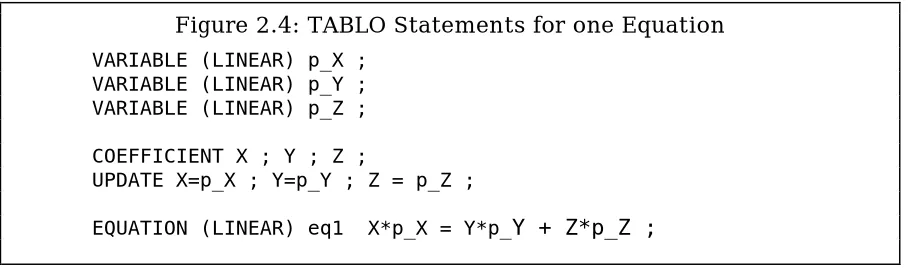
Often linearized equations involve both linear variables and levels variables. For example, the linearized version of the levels equation
X = Y + Z
would often be written as
X*p_X = Y*p_Y + Z*p_Z.
If this linearized equation were written in a linearized TABLO Input file, the percentage changes p_X,p_Y,p_Z would be declared as linear variables and the levels variables would be declared as COEFFICIENTs, as shown in Figure 2.4.
Figure 2.4: TABLO Statements for one Equation
VARIABLE (LINEAR) p_X ; VARIABLE (LINEAR) p_Y ; VARIABLE (LINEAR) p_Z ; COEFFICIENT X ; Y ; Z ;
UPDATE X=p_X ; Y=p_Y ; Z = p_Z ;
EQUATION (LINEAR) eq1 X*p_X = Y*p_Y + Z*p_Z ;
In such a case, the software must be told explicitly the connection between the linear variables and their associated levels variables (COEFFICIENTs). This is done via so-called UPDATE statements. For example, the statement
UPDATE X = p_X ;
in Figure 2.4 indicates that p_X denotes the percentage change in the levels variable X.6 Similarly,
UPDATE (CHANGE) W = c_W ;
would indicate that the linear variable c_W represents the change in levels variable (COEFFICIENT) W.
In linearized TABLO Input files (see, for example, ORANI-F in Horridge et al.
(1993)),
• dollar values are read in but levels of prices and quantities do not usually need to be considered explicitly,
• percentage changes in prices and quantities are explicit linear variables but percentage changes in the associated dollar values are usually not included.
In such files, the dollar values read must be updated via the associated linear price and quantity variables. Most update statements are of the form
UPDATE DV = p * q;
where DV is a COEFFICIENT holding a dollar value and p and q are linear variables denoting percentage changes in the relevant price and quantity.7
2.5 Different Representations (Levels, Linearized or Mixed)
As indicated above, an economic model can be specified by giving all levels equations, all linearized equations or a mixture of linearized and levels equations. In the Stylized Johansen TABLO Input file we used a mixed representation.
For discussions of the merits of working with different representations of models, see Harrison et al. (1993) and Hertel et al. (1992). Since they all produce the same results, our main advice is to work with whichever representation seems most natural or convenient.
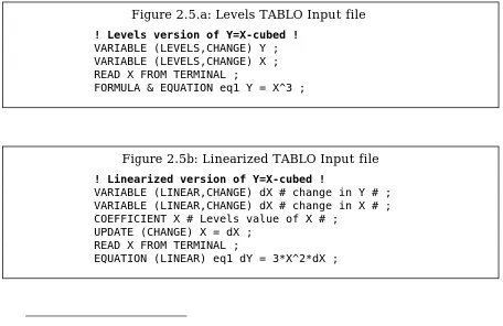
Here, to help reinforce the difference between possible representations, we take the simple (non-economic) example with just one equation Y=X3 , and give both a levels and a linearized TABLO Input file for this (see Figures 2.5a and 2.5b). (Of course, a mixed one is not possible since this is just a single
Figure 2.5.a: Levels TABLO Input file
! Levels version of Y=X-cubed !
VARIABLE (LEVELS,CHANGE) Y ; VARIABLE (LEVELS,CHANGE) X ; READ X FROM TERMINAL ;
FORMULA & EQUATION eq1 Y = X^3 ;
Figure 2.5b: Linearized TABLO Input file
! Linearized version of Y=X-cubed !
VARIABLE (LINEAR,CHANGE) dX # change in Y # ; VARIABLE (LINEAR,CHANGE) dX # change in X # ; COEFFICIENT X # Levels value of X # ;
UPDATE (CHANGE) X = dX ; READ X FROM TERMINAL ;
EQUATION (LINEAR) eq1 dY = 3*X^2*dX ;
7 This UPDATE statement gives rise to the formula new_DV = old_DV[1 + (p+q)/100]
equation.) In these files, “eq1" is the name by which the equation is known in the TABLO Input file. We have chosen to use change variables in both cases since it is quite possible for X and Y to be positive, zero or negative. The initial solution is treated differently in the two cases.
• In the levels case, X is read from the terminal and the initial value of Y is given by the FORMULA (which is also the EQUATION).
• In the linearized case, the initial value of X is read. Although X appears explicitly in the linearized equation in Figure 2.5b, Y does not, and so we do not need to declare a COEFFICIENT Y in this case (or give it initial values).
2.5.1 TABLO Linearizes Levels Equations
When the program TABLO processes a TABLO Input file, it automatically linearizes any levels equations; indeed TABLO converts the whole TABLO Input file to a linearized TABLO Input file (which is called the associated linearized TABLO Input file). After this, all interaction with the software about the model proceeds as if this associated linearized TABLO Input file were the actual TABLO Input file.8 For example, if we begin from the levels TABLO Input file in Figure
2.5a above, when we specify the closure, we must refer to the linear variables c_X and c_Y rather than the levels ones.
When producing the associated linearized file, TABLO inserts UPDATE statements as required to connect the linear and levels variables. For example, when the file in Figure 2.5a above is processed, the statement
UPDATE(CHANGE) X = c_X ;
would be included in the associated linearized TABLO input file.
2.6 Example Models
The following models are usually supplied with GEMPACK:
Stylized Johansen (see Chapter 3 of Dixon et al. (1992)),
Miniature ORANI, a pedagogical model designed to introduce some of the essential ideas behind the ORANI model of the Australian economy (see sections 3-9 of Dixon et al. (1982)),
TRADMOD, a flexible multi-country trade model documented in Hertel et al.
(1992),
ORANI-F, the forecasting version of the ORANI model of the Australian economy, as documented in Horridge et al. (1993),
GTAP, the Global Trade Analysis Project's model for analysing trade issues, as documented in Hertel and Tsigas (1993),
DMR, the well-known Dervis, De Melo, Robinson model of Korea, as documented in Chapter 4 of Dixon et al. (1992),
and three intertemporal models
TREES, a stylized model of forestry designed to show how intertemporal models are implemented within GEMPACK, described in Codsi et al. (1992), CRTS, a single sector investment model, described in Wilcoxen (1989) or Exercises 5.1-5.4 of Chapter 5 of Dixon et al. (1992), and
5SECT, a 5 sector investment model designed as an introduction to the issues involved in building and solving intertemporal models, also described in Wilcoxen (1989) or Part C of Problem Set 5 of Dixon et al. (1992).
Other models implemented and solved via GEMPACK include
• single-country models of the Philippines (Warr et al. (1993) and Borrell
et al. (1994)), Indonesia (Trewin et al. (1993)), Zimbabwe (Quirke et al.
(1993)), Sri Lanka (Centre for International Economics (1992)), China (Gao (1993), Huang (1993) and Martin (1991)), Papua New Guinea (National Centre for Development Studies (1990) and Woldekidan (1993)),
• several extensions of ORANI including FH-ORANI (Dee (1989)), MONASH (Adams et al. (1993)), and a fully intertemporal version (Malakellis (1992)),
• multi-country models such as SALTER (Jomini et al. (1991)), Asian models (Hughes (1990), Mai (1993), Suphachalasai (1989) and Yang (1994)) and an intertemporal model of the global meat industry (Harris
et al. (1992)), and
• an intertemporal model of a Ramsey Problem (McDougall (1994)).
GEMPACK has also been used for database manipulation as in the FIT facility (James et al. (1993)).
GEMPACK software makes it easy to transfer models between different computers (including different operating systems). For example, the main theory of the model is all in the TABLO Input file which is an ASCII text file readily transferred to other computers. Hence it is easy to obtain models from other modellers using GEMPACK (see section 8 below).
3 CARRYING OUT SIMULATIONS
In this section, we describe how simulations are carried out in GEMPACK and how simulation results are reported and interpreted. We illustrate these general points by considering, in some detail, a simulation with Stylized Johansen.
3.1 Interpreting The Results Of A Simulation
When a simulation is carried out, the software typically reports changes or percentage changes in selected variables and produces updates (that is, post-simulation) data. The initial (that is, pre-post-simulation) data is also important in interpreting results. We illustrate these points by taking an example simulation with Stylized Johansen.
3.1.1 A Simulation With Stylized Johansen
simulation in which the supply of labor is increased by 10 per cent and the supply of capital is held fixed.
We have taken the initial data to be as in Table E3.3.1 of DPPW; we reproduce this here as Table 3.1.1a. For example, households consume 4 (million) dollars' worth of commodity 2 and industry 2 uses 3 (million) dollars' worth of labor. The amounts in the last row and column are totals.
Table 3.1.1a: Input-output Data Base for Stylized Johansen
Sectors Households Total Sales 1 2
Commodity 1 4.0 2.0 2.0 8.0
Sectors
Commodity 2 2.0 6.0 4.0 12.0
Labor 3 1.0 3.0 4.0
Factors
Capital 4 1.0 1.0 2.0
Total Production 8.0 12.0 6.0
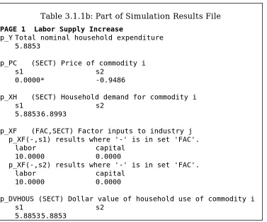
Some of the results of this simulation are given in Table 3.1.1b. (This shows the values of certain of the endogenous variables essentially in the form output by the GEMPACK program GEMPIE.)
Table 3.1.1b: Part of Simulation Results File
PAGE 1 Labor Supply Increase
p_Y Total nominal household expenditure 5.8853
p_PC (SECT) Price of commodity i s1 s2
0.0000* -0.9486
p_XH (SECT) Household demand for commodity i
s1 s2
5.8853 6.8993
p_XF (FAC,SECT) Factor inputs to industry j p_XF(-,s1) results where '-' is in set 'FAC'.
labor capital 10.0000 0.0000
p_XF(-,s2) results where '-' is in set 'FAC'. labor capital
10.0000 0.0000
p_DVHOUS (SECT) Dollar value of household use of commodity i
s1 s2
5.8853 5.8853
(1) households will consume 6.8993 per cent more of commodity 2 than they did previously (the 'p_XH' result for commodity 2),
(2) the price of commodity 2 will fall by 0.9486 per cent (the 'p_PC' result for commodity 2), and
(3) the dollar value of household consumption of commodity 2 will rise by 5.8853 per cent (the p_DVHOUS("s2") result).
Recall that, in the TABLO Input file for Stylized Johansen (see section 2.3.1), initial levels values of prices and quantities are calculated by setting prices to 1, which just sets the units in which quantities are measured. Then, for example, since households consume 4 million dollars' worth of commodity 2, this means that they consume 4 million units of that commodity.
Hence the three simulation results mentioned above mean that, once labor is increased by 10 per cent and capital is held fixed,
(1) household consumption of commodity 2 has increased to 4.2760 million units (6.8993 per cent more than the original 4 million units), (2) the price of commodity 2 has fallen from one dollar per unit to
approximately 99.051 cents per unit (a fall of 0.9486 per cent), and (3) the dollar value of household consumption of the commodity produced
by sector "s2" has risen from 4 million dollars to approximately 4.2354 million dollars (an increase of 5.8853 per cent).
Of course the updated values in (1), (2) and (3) above should be related since dollar value should equal price times quantity. Note that this is true since, from (1) and (2) above, the post-simulation price times the post-simulation quantity is
0.99051 x 4.2760 = 4.2354
which is indeed the post-simulation dollar value in (3). This confirms that the solution shown in the results file satisfies the levels equation connecting price, quantity and dollar value of household consumption of this commodity.
From the results of the simulation, it is easy to infer the new levels values of all quantities of interest in the model (prices, quantities and dollar values). Indeed, the updated data file produced during the simulation contains the new levels values for the quantities read in initially from the data base.
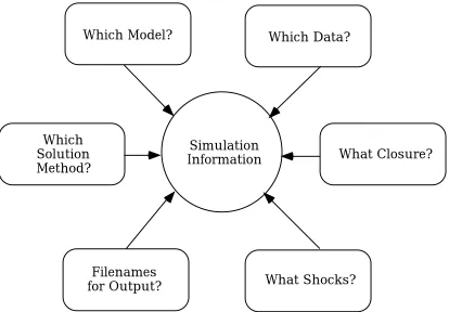
3.2 Specifying A Simulation
In order to specify the details for carrying out a simulation, it is necessary to give details of
• which model to use,
• which base data to begin from (the pre-simulation solution),
• the closure (the endogenous and exogenous variables),
• the variables to shock, and by how much, and
• the names of the various output files.
Which Model?
Which Data?
What Closure?
Simulation
Information
Which
Solution
Method?
Filenames
for Output?
What Shocks?
Figure 3.2: The Information Required to Specify a Simulation
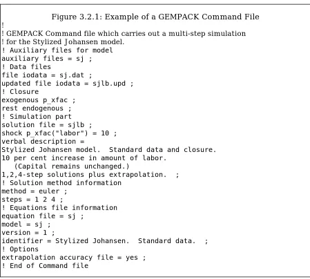
GEMPACK uses small text files called Command files to specify a simulation. The Command file used to specify the simulation described in section 3.1.1 above is shown in full in Figure 3.2.1; we describe some of its features in section 3.2.1 below. The syntax of Command files has been chosen in the hope of providing an easily understood and self-contained record of the simulation.9
3.2.1 An Example Command File
The statement
auxiliary files = sj ;
in the Command file shown in Figure 3.2.1 tells the program carrying out the simulation which model to work with, since these auxiliary files are just a processed version of the TABLO Input file for the Stylized Johansen model (see section 3.3 below). The statement
file iodata = sj.dat ;
tells the program to read base data from the file SJ.DAT (which contains the data in Table 3.1.1a above). The statements
exogenous p_xfac ; rest endogenous ;
give the closure (that is, which variables to take as exogenous and which to take as endogenous), while the statement
shock p_xfac("labor") = 10 ;
describes the shock to increase the supply of labor by 10 per cent.
Figure 3.2.1: Example of a GEMPACK Command File
!
! GEMPACK Command file which carries out a multi-step simulation ! for the Stylized Johansen model.
! Auxiliary files for model auxiliary files = sj ; ! Data files
file iodata = sj.dat ;
updated file iodata = sjlb.upd ; ! Closure
exogenous p_xfac ; rest endogenous ; ! Simulation part solution file = sjlb ;
shock p_xfac("labor") = 10 ; verbal description =
Stylized Johansen model. Standard data and closure. 10 per cent increase in amount of labor.
(Capital remains unchanged.)
1,2,4-step solutions plus extrapolation. ; ! Solution method information
method = euler ; steps = 1 2 4 ;
! Equations file information equation file = sj ;
model = sj ; version = 1 ;
identifier = Stylized Johansen. Standard data. ; ! Options
extrapolation accuracy file = yes ; ! End of Command file
The statement
solution file = sjlb ;
specifies the name of the Solution file to contain the solution of the simulation. The statement
updated file iodata = sjlb.upd ;
names the file to contain the updated (that is, post-simulation) data. (The name includes 'LB' to remind us that this data depends on the labor shock.) The verbal description of the simulation, which can be several lines of text, goes on the
verbal description = ... ;
gives 4 lines of text for the verbal description in this case. (The ';' indicates the end of this description. Note that all statements in GEMPACK Command files must end with a semicolon';'. Lines beginning with an exclamation mark ! are comments.)
With GEMPACK, there are 4 related solution methods one of which can be chosen for a simulation. These are introduced in section 4.3 below. The statements
method = euler ; steps = 1 2 4 ;
tell the program to use Euler's method based on 3 separate solutions using 1, 2 and 4 steps respectively. The accuracy of the solution depends on the solution method and the numbers of steps. The statement
extrapolation accuracy file = yes ;
asks the program to produce a so-called Extrapolation Accuracy file which
provides information about the accuracy of the solution (see section 4.3 for more details).
The program carrying out the simulation usually produces a so-called
Equations file (see section 4.1 below) which contains the numerical linearized
equations of the model. (This can be used as a starting point for calculating Johansen solutions - see section 4.4 below.) The statements
equations file = sj ; model = sj ;
version = 1 ;
identifier = Stylized Johansen. Standard data. ;
specify the name of the Equations file, the model name, the version number and a model identifier.
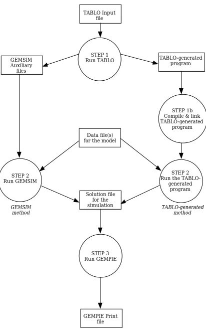
3.3 Steps In Carrying Out A Simulation
The program GEMSIM is a general-purpose program for carrying out simulations with different models. It can be used to carry out simulations with any model implemented in GEMPACK.
TABLO Input file
STEP 1 Run TABLO GEMSIM
Auxiliary files
STEP 2 Run GEMSIM
Data file(s) for the model
TABLO-generated program
STEP 1b Compile & link TABLO-generated
program
STEP 2 Run the
TABLO-generated program Solution file
for the simulation
STEP 3 Run GEMPIE
GEMPIE Print file
Figure 3.3: Steps in carrying out a Simulation
GEMSIM method
The GEMSIM method of carrying out simulations is illustrated on the left hand side of Figure 3.3 while the TABLO-generated method is on the right hand side.10 The three steps are:
Step 1. Computer Implementation of the Model
Process the TABLO Input file for the model by running the GEMPACK program TABLO. The user can choose either the GEMSIM method or TABLO-generated program method. If the TABLO-generated program route is chosen, after TABLO has finished, the TABLO-generated program is compiled using an appropriate Fortran compiler, and linked to the GEMPACK library of subroutines.
Step 2. Simulation
Run the GEMPACK program GEMSIM or the TABLO-generated program. Specify which base data are to be read and describe the closure (that is, the exogenous and endogenous variables) and the shocks as described in section 3.2. The program then computes the solution to the simulation and writes the results to a so-called Solution file. It also produces updated data.
Step 3. Printing the Results of the Simulation
Run the GEMPACK program GEMPIE to convert the solution produced in Step 2 to a so-called GEMPIE Print file. This is a text file which can be printed (or edited).
Often many different simulations are carried out on the same model, for example, with different closures and/or shocks, or starting from different base data. In these cases, Steps 2 and 3 are repeated but not Step 1. However Step 1 must be repeated if the TABLO Input file for the model is changed in any way.
The input to specify a simulation is essentially the same for both GEMSIM and the TABLO-generated program. Command files, as in section 3.2, can be used for both. These programs can also be run interactively by responding to prompts from the program.
3.4 Different Closures And Shocks
Most general equilibrium models have several different closures; which one to use depends on the purpose of the simulation in question. In section 3.4.1 below, we show how different closures can be specified on a GEMPACK Command file.
Especially when the model is used for forecasting, a large number of shocks may need to be specified. In section 3.4.2 below, we show how these can be specified on a GEMPACK Command file.
3.4.1 Different Closures
With the Stylized Johansen model, the usual closure has supplies of the 2 primary factors (labor and capital) exogenous and all other variables endogenous. Alternative closures are to have the supply of one factor and the price of the other factor exogenous and all other variables endogenous. The statements in a Command file for the first of these closures can be
exogenous p_xfac ; rest endogenous ;
(as shown in Figure 3.2.1) while the statements
exogenous p_XFAC("labor") p_PF("capital") ; rest endogenous ;
specify the closure in which the supply of labor and the price of capital are exogenous.
With large general-purpose models such as ORANI-F (see Horridge et al.
(1993)) or GTAP (see Hertel and Tsigas (1993)), there are usually a large number of different closures. For example, in ORANI-F (see section 5 of Horridge et al.
(1993)),
(a) the numeraire can be either the exchange rate 'phi' or the domestic CPI 'p3tot';
(b) it may be appropriate to take aggregate employment 'employ_i' exogenous and the real wage rate endogenous, or vice versa;
(c) it may be appropriate to exogenise household consumption (via the variable 'w3lux') or to exogenise the balance of trade (via variable 'delB').
The usual (general equilibrium) closure of GTAP has supplies of land, labor and capital exogenous (in all regions) and supplies of all other commodities and all commodity prices endogenous. It is also useful to consider partial equilibrium closures to illustrate differences between policies and/or to analyse different policies. In one such closure, a multi-region general-equilibrium (MRGE) closure in the GTAP literature focusing on food (see Hertel and Tsigas (1993)), supplies of all commodities except food in all regions are exogenous and all commodity prices except for those of food and land in all regions are exogenous; with this closure some equations which usually hold in a general equilibrium model are effectively turned off to give a partial equilibrium model. Usually the variable 'walraslack' is endogenous and its value is used to check that Walras law holds; in the MRGE closure mentioned above, this variable is set exogenous (and not shocked) in order to ensure that Walras law still holds in this partial-equilibrium version of the model.
On a GEMPACK Command file, the usual way of specifying a closure is to list the exogenous variables and to conclude with the statement “rest endogenous ;".
modify closure on Environment file orf ; swap p3tot = phi ;
swap delB = w3lux ;
using "swap" statements or, alternatively,
modify closure on Environment file orf ; exogenous p3tot delB ;
endogenous phi w3lux ;
in which the new status of the relevant variables is indicated explicitly.
3.4.2 Shocks
The values of shocks can appear directly on a Command file or on a text file whose name is given on the Command file. For example, for the ORANI-F simulation discussed in section 7 of Horridge et al.(1993), the Command file may contain statements
shock p3tot = 34.01 ;
shock delx6 = file delx6.shk ; shock pf0cif = uniform 23.64 ;
The first line gives the shock to the domestic CPI 'p3tot'; it says that this should be increased by 34.01 per cent. The second line says that the values of the shocks to the 13 different components of variable 'delx6' (changes in stocks in the 13 different sectors) can be read from the text file 'delx6.shk'. The third line says that the same shock (this is what the word 'uniform' means), namely an increase of 23.64 per cent, should be given to each of the 13 components of variable 'pf0cif'; these shocks are part of the changes in the terms of trade expected over the period covered by the forecast.
In some cases, values of shocks may be calculated most easily via a TABLO Input file constructed explicitly for this purpose. For example, with GTAP, it is convenient to construct a TABLO Input file which reads the existing data, calculates current distortions and then calculates changes required to remove these distortions; these values can be written to text files (using WRITE statements). These text files can serve as the shock files for simulations with the model intended to give information about changes once some or all of the distortions are removed (for example, after various GATT policy changes are implemented by some or all countries).
4 HOW GEMPACK SOLVES THE EQUATIONS
We first describe how approximate solutions, know as Johansen solutions, are calculated. This leads on to accurate multi-step solutions, and then to the different solution methods available within GEMPACK. Finally, in section 4.4, we describe how the GEMPACK program SAGEM can calculate several Johansen solutions simultaneously.
4.1 Johansen Solutions
C z = 0 (1) where
C is the m x p matrix of coefficients of the equations, z is the p x 1 vector of all the variables of the model,
m is the total number of equations,
p is the total number of variables.
In general, m is less than p in the system of equations in (1) above, so in a simulation (Johansen or multi-step),
(p -m) of the variables are exogenous,
the remaining m variables are endogenous, and
shocks (usually percentage changes) are given to some of the exogenous variables.
For example, for Stylized Johansen, the total number of variables p is 29 and the total number of equations m is 27, so we need 2 exogenous variables. We can shock either 1 or 2 of these exogenous variables.
Once the exogenous/endogenous split has been chosen, the system of equations Cz = 0, as in (1) above, becomes
A.z1 = –D.z2 (2)
where z1 and z2 are respectively the (column) vectors of endogenous and exogenous variables, A is m x m and D is m x (p-m). The columns of the matrices A and D are just the columns of C corresponding to the endogenous and exogenous variables respectively. The shocks are the values to use for z2 . Once these are known, we have a system
A.z1 = b (3)
to solve (where b is an m x 1 vector). It is the solution z1 of this matrix equation (3) which is the Johansen solution11 of the simulation.12
Because the levels equations of the model are usually nonlinear, the results of this calculation are only approximations (sometimes good ones and sometimes not-so-good ones) to the corresponding solution of the levels equations of the model. Accurate solutions require multi-step calculations, which we now describe.
4.2 Multi-Step Solutions
The idea of a multi-step simulation is to break each of the shocks up into several smaller pieces. In each step, the linearized equations are solved for these smaller shocks. After each step the data, shares and elasticities are recalculated to take into account the changes from the previous step.
11 This name pays tribute to Johansen who pioneered this way of obtaining useful approximate solutions of general equilibrium solutions around 1960.
Figure 4.2 below makes this easy to visualize. In that figure we consider just one exogenous variable X (shown on the horizontal axis) and one endogenous variable Y (vertical axis); these are constrained to stay on the curve g(X,Y) = 0. We suppose that they start from initial values X0 ,Y0 at the point A and that X is shocked from value X0 to value X1 . Ideally we should follow the curve g(X,Y)=0 in solving this. In a Johansen (that is, a 1-step) solution we follow the straight line which is a tangent to the curve at point A to reach point BJ and so get solution YJ .
Y
J
E2
0
X
1
g
= 0
B
C
2
A
Y
Y
Y
Y
X
X
(X, Y)
B
B
2J
1 0
Figure 4.2: Multi-step solution using Euler's method
•
•
•
In Euler's method the direction to move at each step is essentially that of the tangent to the curve at the appropriate point. In a 2-step Euler solution (see Figure 4.2), we first go half way along this tangent to point C2 , then recompute the direction in which to move, and eventually reach point B2 , giving solution YE2 . The exact solution is at B where Y has value Y1 . In a 4-step Euler
simulation we follow a path of 4 straight-line segments, and so on for more steps.
In general, the more steps the shocks are broken into, the more accurate will be the results.
4.3 Solution Methods And Extrapolation
One way of increasing accuracy of solution is to increase the number of steps in a multi-step solution. It turns out however that the best way to obtain an accurate solution is to carry out 2 or 3 different multi-step calculations with different numbers of steps and then to calculate the solution as an appropriate weighted average of these; this is what is meant by the extrapolated solution.
direction in which to move at each step. When the shocks are broken into N parts, Euler's method does N separate calculations while Gragg's method does N+1. Usually the computational cost of this extra calculation is more than repaid by the extra accuracy obtained. (The midpoint method is similar to Gragg’s method.)
To illustrate these points, we show below the different results for the percentage change in household expenditure 'p_Y' in the Stylized Johansen model for the simulation in section 3.1 above, in which labor supply is increased by 10 per cent and capital remains infixed supply. Table 4.3 shows Euler and Gragg results for different step numbers and extrapolations based on them. Note that the exact result is 5.88528.
Table 4.3: Multistep and Extrapolated Results
Multi-step results for different methods and step numbers
Method Number of steps
1 2 4 6 100
Euler 6.00000 5.94286 5.91412 5.90452 5.88644 Gragg13 5.88675 5.88545 5.88529
Extrapolated results
From Euler 1,2-step results 5.88571 From Euler 1,2,4-step results 5.88527 From Gragg 2,4,6-step results 5.88529
Note that, in this case, the 4-step Gragg result is more accurate than the 100-step Euler result and that the result extrapolated from 1,2,4-step Euler results is much more accurate than the 100-step Euler result (even though the latter takes about 100/7 times as long to compute). These results are typical of what happens in general.
The general messages are:
1. Gragg's method is usually much more accurate than Euler's. 2. If in doubt, extrapolate.
3. Extrapolating from 3 different solutions is better than from 2. (For example, extrapolating from Gragg 2,4 and 6-step solutions is usually better than from just 4 and 6-step solutions.)
An Extrapolation Accuracy file can be produced to show how accurate the solution is for each endogenous variable. The separate columns show the results
for the different multi-step solutions calculated, and the last column of results is the extrapolated result. When 3 different multi-step results are used for extrapolation (which is what we recommend), the last two columns give conservative information about the number of figures of accuracy of each result.
4.3.1 Connection With Initial Value Problems
The kind of simulations GEMPACK is designed to solve can be converted to a class of well-known problems called Initial Value problems. Details of this conversion are given in Appendix B.
There are many different methods for solving Initial Value problems, as can be seen by consulting almost any numerical analysis textbook, for example, Chapter 6 of Atkinson (1989). GEMPACK makes available three of the simplest and best-known methods, namely Euler’s method, the midpoint method and Gragg's method (also known as the modified midpoint method); see, for example, Chapter 6 of Atkinson (1989) or Chapter 15 of Press et al. (1986) for a description of these methods. All of these methods solve an Initial Value problem by approximating the solution curve by a sequence of straight-line segments, as in Figure 4.2 above.
Different Initial Value solution methods have different orders of errors. Euler is an order 1 method in the sense that, if the number of steps is multiplied by N, then the errors are approximately divided by N, while Gragg and midpoint are order 2 methods which means that the errors are approximately divided by N2 .
Within GEMPACK, we recommend extrapolating from three different solutions (each calculated with a different number of steps - for example, 2,4,6-step solutions); this is usually the most efficient way of obtaining accurate solutions of Initial Value problems. When extrapolating from three solutions using Euler's method, if the number of steps are all multiplied by N, then the errors in the extrapolated solution will be divided approximately by N3 . (For example, the errors in the result extrapolated from 6,12,18-step Euler solution is expected to be twenty-seven times smaller than that from a 2,4,6-step Euler solution; here N=3.) For Gragg and the midpoint method, the errors in the extrapolated result are expected to be divided by N6 (instead of N3 for Euler) . See, for example, Atkinson (1989) or Press et al. (1986) for details about general extrapolation errors; see Pearson (1991) for a discussion with reference to GEMPACK solution methods.
4.4 Several Johansen Simulations At Once
The GEMPACK program SAGEM can be used to compute several Johansen solutions at once. Although Johansen solutions are less accurate than multi-step ones, carrying out Johansen simulations can be quite revealing. In many cases, the results are sufficiently accurate to produce the right qualitative results. Being able to compute several such solutions more quickly than one multi-step solution has its advantages, especially for a new model whose behaviour you are just beginning to understand.