Noname manuscript No.
(will be inserted by the editor)
A new class of irreducible pentanomials for
polynomial based multipliers in binary fields
Gustavo Banegas · Ricardo Cust´odio ·
Daniel Panario
the date of receipt and acceptance should be inserted later
Abstract We introduce a new class of irreducible pentanomials over F2 of the form f(x) = x2b+c+xb+c+xb+xc+ 1. Let m = 2b+c and use f to define the finite field extension of degree m. We give the exact number of operations required for computing the reduction modulof. We also provide a multiplier based on Karatsuba algorithm inF2[x] combined with our reduction process. We give the total cost of the multiplier and found that the bit-parallel multiplier defined by this new class of polynomials has improved XOR and AND complexity. Our multiplier has comparable time delay when compared to other multipliers based on Karatsuba algorithm.
Keywords irreducible pentanomials· polynomial multiplication· modular reduction· finite fields
1 Introduction
Finite field extensions F2m of the binary fieldF2 play a central role in many
engineering applications and areas such as cryptography. Elements in these extensions are commonly represented using polynomial or normal bases. We center in this paper on polynomial bases for bit-parallel multipliers.
When using polynomial bases, since F2m ∼= F2[x]/(f) for an irreducible
polynomial f overF2 of degree m, we write elements inF2m as polynomials
overF2 of degree smaller than m. When multiplying with elements inF2m, a
polynomial of degree up to 2m−2 may arise. In this case, a modular reduc-tion is necessary to bring the resulting element back toF2m. Mathematically,
any irreducible polynomial can be used to define the extension. In practice,
however, the choice of the irreducible f is crucial for fast and efficient field multiplication.
There are two types of multipliers inF2m: one-step algorithms and two-step
algorithms. Algorithms of the first type perform modular reduction while the elements are being multiplied. In this paper, we are interested in two-step algo-rithms, that is, in the first step the multiplication of the elements is performed, and in the second step the modular reduction is executed. Many algorithms have been proposed for both types. An interesting application of two-step algo-rithms is in several cryptographic implementations that use the lazy reduction method [23, 2]. For example, in [15] it is shown the impact of lazy reduction in operations for binary elliptic curves. An important application of the second part of our algorithm, the reduction process, is to side-channel attacks. Indeed, we prove that our modular reduction requires a constant number of arithmetic operations, and as a consequence, it prevents side-channel attacks.
The complexity of hardware circuits for finite field arithmetic in F2m is
related to the amount of space and the time delay needed to perform the operations. Normally, the number of exclusive-or (XOR) and AND gates is a good estimation of the space complexity. The time complexity is the delay due to the use of these gates.
Several special types of irreducible polynomials have been considered be-fore, including polynomials with few nonzero terms like trinomials and pen-tanomials (three and five nonzero terms, respectively), equally spaced poly-nomials, all-one polynomials [6, 11, 19], and other special families of polynomi-als [27]. In general, trinomipolynomi-als are preferred, but for degrees where there are no irreducible trinomials, pentanomials are considered.
The analysis of the complexity using trinomials is known [26]. However, there is no general complexity analysis of a generic pentanomial in the lit-erature. Previous results (see [4] for details) have focus on special classes of pentanomials, including:
– xm+xb+1+xb+xb−1+ 1, where 2≤b≤m/2−1 [10, 20, 28, 18, 8];
– xm+xb+1+xb+x+ 1, where 1< b < m−1 [9, 19, 20, 28, 18, 8];
– xm+xm−c+xb+xc+ 1, where 1≤c < b < m−c [3];
– xm+xa+xb+xc+ 1, where 1≤c < b < a≤m/2 [19];
– xm+xm−s+xm−2s+xm−3s+ 1, where (m−1)/8≤s≤(m−1)/3 [19];
– x4c+x3c+x2c+xc+ 1, wherec= 5iand i≥0 [6, 7].
1.1 Contributions of this paper
In this paper, we introduce a new class of irreducible pentanomials with the following format:
f(x) =x2b+c+xb+c+xb+xc+ 1, b > c >0. (1)
We compare our pentanomial with the first two families from the list above. The reason to choose these two family is that [18] presents a multiplier consid-ering these families with complexity 25% smaller than the other existing works in the literature using quadratic algorithms. Since our multiplier is based on Karatsuba’s algorithm, we also compare our method with Karatsuba type al-gorithms.
An important reference for previously used polynomials and their com-plexities is the recent survey on bit-parallel multipliers by Fan and Hasan [4]. Moreover, we observe that all finite fields results used in this paper can be found in the classical textbook by Lidl and Niederreiter [12]; see [14] for recent research in finite fields.
We prove that the complexity of the reduction depends on the exponentsb
andcof the pentanomial. A consequence of our result is that for a given degree
m = 2b+c, for any positive integers b > c >0, all irreducible polynomials in our family have the same space and time complexity. We provide the exact number of XORs and gate delay required for the reduction of a polynomial of degree 2m−2 by our pentanomials. The number of XORs needed is 3m−2 = 6b + 3c−2 when b 6= 2c; for b = 2c this number is 125m−1 = 12c−1. We also show that AND gates are not required in the reduction process. It is easy to verify that our reduction algorithm is “constant-time” since it runs the same amount of operations independent of the inputs and it avoids timing side-channel attacks [5].
For comparison purposes with other pentanomials proposed in the litera-ture, since the operation considered in those papers is the product of elements inF2m, we also consider the number of ANDs and XORs used in the
multipli-cation prior to the reduction. In the literature, one can find works that use the standard product or use some more efficient method of multiplication, such as Karatsuba, and then add the complexity of the reduction.
In this paper, we use a Karatsuba multiplier combined with our fast reduc-tion method. The total cost is thenCmlog23+ 3m−2 orCmlog23+12
1.2 Structure of the paper
The structure of this paper is as follows. In Section 2 we give the number of required reduction steps when using a pentanomial f from our family. We show that for our pentanomials this number is 2 or 3. This fact is crucial since such a low number of required reduction steps of our family allows for not only an exact count of the XOR operations but also for a reduced time delay. Our strategy for that consists in describing the reduction process throughout equa-tions, cleaning the redundant operations and presenting the final optimized algorithm. Section 3 provides the first component of our strategy. In this sec-tion, we simply reduce a polynomial of degree at most or exactly 2m−2 to a polynomial of degree smaller thanm. The second component of our strategy is more delicate and it allows us to derive the exact number of operations in-volved when our pentanomialf is used to defineF2m. Sections 4 and 5 provide
those analyses for the cases when two and three steps of reduction are needed, that is, when c = 1 and c > 1, respectively. We give algorithms and exact estimates for the space and time complexities in those cases. Also, we describe a Karatsuba multiplier implementation combined with our reduction. In Sec-tion 6, based on our implementaSec-tion, we show that the number of XOR and AND gates is better than the known space complexity in the literature. On the other hand, the time complexity (delay) in our implementation is worse than quadratic methods but comparable with Karatsuba implementations. Hence, our multiplier would be preferable in situations where space complexity and saving energy are more relevant than time complexity. We demonstrate that our family contains many polynomials, including degrees where pentanomials are suggested by NIST. Conclusions are given in Section 7.
2 The number of required reductions
When operating with two elements in F2m, represented by polynomials, we
obtain a polynomial of degree at most 2m−2. In order to obtain the corre-sponding element inF2m, a further division with remainder by an irreducible
polynomial f of degree m is required. We can see this reduction as a pro-cess to bring the coefficient in interval [2m−2, m] to a position less thanm. This is done in steps. In each step, the coefficients in interval [2m−2, m] of the polynomial is substituted by the equivalent bits following the congruence
xm≡xa+xb+xc+ 1. Once the coefficient in position 2m−2 is brought to a position less thanm, the reduction is completed.
Let D0(x) =
P2m−2
i=0 dixi be a polynomial over F2. We want to compute Dred, the remainder of the division ofD0 byf, wheref has the formf(x) = x2b+c+xb+c+xb+xc+ 1 with 2b+c = m and b > c > 0. The maximum numberkaof reduction steps for a pentanomialxm+xa+xb+xc+ 1 in terms of the exponentais given by Sunar and Ko¸c [22]
ka=
m−2
m−a
+ 1.
In our casem= 2b+c anda=b+c, thus
kb+c=
2b+c−2 2b+c−b−c
+ 1 =
c−2 b
+ 3 =
(
2 ifc= 1,
3 ifc >1. (2)
Using the same method as in [22], we can derive the number of steps required associated to the exponents band c. These numbers are needed in Section 3. We get
kb=
2b+c
−2 2b+c−b
+ 1 = b
−2
b+c
+ 2 = 2, (3)
and
kc =
2b+c−2 2b+c−c
+ 1 = c−2
2b
+ 2 = (
1 ifc= 1,
2 ifc >1. (4)
Thus, the reduction process for our family of pentanomials involves at most three steps. This is a special property that our family enjoys.
The general process for the reduction proposed in this paper is given in the next section. The special case c = 1, that is when our polynomials have the formf(x) =x2b+1+xb+1+xb+x+ 1, requires two steps. This family is treated in detail in Section 4. The general case of our family f(x) =x2b+c+
xb+c+xb+xc+ 1 forc >1 involves three steps and is treated in Section 5.
3 The general reduction process
The general process that we follow to get the original polynomialD0reduced to a polynomial of degree smaller than m is depicted in Figure 1. Without loss of generality, we consider the polynomial to be reduced as always having degree 2m−2. Indeed, the cost to determine the degree of the polynomial to be reduced is equivalent to checking if the leading coefficient is zero.
D0 = A0 B0
A1 B1
A2 B2
A3 B3
+
+
+
+ D1 =
D2 =
D3 =
Fig. 1 Tree representing the general reduction strategy.
3.1 DeterminingA0 andB0
We trivially have
D0(x) =A0(x) +B0(x) = 2m−2
X
i=m
dixi+ m−1
X
i=0 dixi,
and hence
A0=
2m−2 X
i=m
dixi and B0=
m−1 X
i=0
dixi. (5)
3.2 DeterminingA1 andB1
Using for clarity the generic form of a pentanomial overF2,f(x) =xm+xa+ xb+xc+ 1, dividing the leading term ofA
0 by f and taking the remainder, we get
D1=
m−2 X
i=0
di+mxi+a+ m−2
X
i=0
di+mxi+b+ m−2
X
i=0
di+mxi+c+ m−2
X
i=0
di+mxi.
Separating the already reduced part of D1 from the piece of D1 that still requires more work, we obtain
A1=
m+a−2 X
i=m
di+(m−a)xi+ m+b−2
X
i=m
di+(m−b)xi+ m+c−2
X
i=m
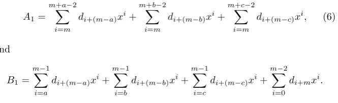
di+(m−c)xi, (6)
and
B1=
m−1 X
i=a
di+(m−a)xi+ m−1
X
i=b
di+(m−b)xi+ m−1
X
i=c
di+(m−c)xi+ m−2
X
i=0
Sincem= 2b+c anda=b+c, we have
A1=
3b+2c−2 X
i=2b+c
di+bxi+ 3b+c−2
X
i=2b+c
di+b+cxi+ 2b+2c−2
X
i=2b+c
di+2bxi,
B1=
2b+c−1 X
i=b+c
di+bxi+ 2b+c−1
X
i=b
di+b+cxi+ 2b+c−1
X
i=c
di+2bxi+ 2b+c−2
X
i=0
di+2b+cxi. (7)
3.3 DeterminingA2 andB2
As before, we divide the leading term ofA1byf and we obtain the remainder D2. We get D2 = D2a +D2b +D2c, where D2a, D2b and D2c refer to the
reductions of the sums in Equation (6). We start withD2a:
D2a=
a−2 X
i=0
di+2m−axi(xa+xb+xc+ 1).
SeparatingD2a in the piecesA2a and B2a, we get A2a =
P2a−2
i=m di+2m−2axi sinceb+a−2< m, and
B2a =
m−1 X
i=a
di+2m−2axi+ a+b−2
X
i=b
di+2m−a−bxi+ a+c−2
X
i=c
di+2m−a−cxi+ a−2 X
i=0
di+2m−axi.
Substitutingm= 2b+canda=b+c, we getA2a =
P2b+2c−2 i=2b+c di+2bx
i, and
B2a =
2b+c−1 X
i=b+c
di+2bxi+ 2b+c−2
X
i=b
di+2b+cxi+ b+2c−2
X
i=c
di+3bxi+ b+c−2
X
i=0
di+3b+cxi.
Proceeding with the reduction now of the second sum in Equation (6), we obtain
D2b =
a+b−2 X
i=a
di+2m−a−bxi+ 2b−2
X
i=b
di+2m−2bxi+ b+c−2
X
i=c
di+2m−b−cxi+ b−2 X
i=0
di+2m−bxi.
Clearly,D2b is already reduced, and thusA2b= 0, and
B2b =
2b+c−2 X
i=b+c
di+2b+cxi+ 2b−2
X
i=b
di+2b+2cxi+ b+c−2
X
i=c
di+3b+cxi+ b−2 X
i=0
di+3b+2cxi.
We finally reduce the third and last sum in Equation (6):
D2c =
a+c−2 X
i=a
di+2m−a−cxi+ b+c−2
X
i=b
di+2m−b−cxi+ 2c−2
X
i=c
di+2m−2cxi+ c−2 X
i=0
Again, we easily check thatD2c is reduced and soA2c = 0, and
B2c=
b+2c−2 X
i=b+c
di+3bxi+ b+c−2
X
i=b
di+3b+cxi+ 2c−2
X
i=c
di+4bxi+ c−2 X
i=0
di+4b+cxi.
Concluding,A2is given by
A2=A2a+A2b+A2c =
2a−2 X
i=m
di+2m−2axi, (8)
andB2=B2a+B2b+B2c is
B2=
2b+c−1 X
i=b+c
di+2bxi+ b+2c−2
X
i=c
di+3bxi+ b+2c−2
X
i=b+c
di+3bxi+ 2c−2
X
i=c
di+4bxi+
2b+c−2 X
i=b
di+2b+cxi+ 2b+c−2
X
i=b+c
di+2b+cxi+ 2b−2
X
i=b
di+2b+2cxi+ b+c−2
X
i=0
di+3b+cxi+
b+c−2 X
i=c
di+3b+cxi+ b+c−2
X
i=b
di+3b+cxi+ b−2 X
i=0
di+3b+2cxi+ c−2 X
i=0
di+4b+cxi.
(9)
3.4 DeterminingA3 andB3
Dividing the leading term ofA2 in Equation (8) byf, we have
D3=
b+2c−2 X
i=b+c
di+3bxi+ b+c−2
X
i=b
di+3b+cxi+ 2c−2
X
i=c
di+4bxi+ c−2 X
i=0
di+4b+cxi.
We have thatD3 is reduced soA3= 0 and
B3=
b+2c−2 X
i=b+c
di+3bxi+ b+c−2
X
i=b
di+3b+cxi+ 2c−2
X
i=c
di+4bxi+ c−2 X
i=0
di+4b+cxi. (10)
3.5 The number of terms inArandBr
Let G(i) = 1 if i > 0 andG(i) = 0 if i≤0. Let r be a reduction step. It is clear now that the precise number of terms forAr andBr, for r≥0, can be obtained usingkb+c,kb andkc given in Equations (2), (3) and (4). We have:
i) The number of terms ofA0 andB0is 1.
4 The family of polynomials f(x) =x2b+1+xb+1+xb+x+ 1
In this section, we consider the case when c = 1, that is, when kb+c = 2, as given in Equation (2). The polynomials in this subfamily have the form
f(x) =x2b+1+xb+1+xb+x+ 1. For the subfamily treated in this section, sincekb+c= 2, we immediately getA2= 0 and the expressions in the previous section simplify. As a consequence, the desired reduction is given by
Dred=B0+B1+B2. Using Equations (5), (7) and (9), we obtain
Dred=
2b X
i=0 dixi+
2b X
i=b+1
di+bxi+ b X
i=1
di+2bxi+ b X
i=1
di+3bxi+ 2b X
i=b
di+b+1xi+
b−1 X
i=0
di+2b+1xi+ 2b−1
X
i=b+1
di+2b+1xi+ 2b−2
X
i=b
di+2b+2xi+ b−2 X
i=0
di+3b+2xi+d3b+1.
(11) A crucial issue that allows us to give improved results for our family of pentanomials is the fact that redundancies occur for Dred in Equation (11). Let
T1(j) = b−2 X
i=0
(di+2b+1+di+3b+2)xi+j, T2(j) =d3bxj,
T3(j) =d3b+1xj, T4(j) = b−1 X
i=0
(di+2b+1+di+3b+1)xi+j.
A careful analysis of Equation (11) reveals that T1,T2 andT3 are used more than once, and hence, savings can occur. We rewrite Equation (11) as
Dred=B0+T1(0) +T1(b) +T1(b+ 1) +T2(b−1)+ T2(2b−1) +T2(2b) +T3(0) +T3(2b) +T4(1).
(12)
One can check that by pluggingT1,T2,T3andT4in Equation (12) we recover Equation (11). Figure 2 shows these operations. We remark that even though the first row in this figure isB0, the following two rows are notB1andB2. In-deed, those rows are obtained fromB1andB2together with the optimizations provided byT1,T2,T3 andT4.
Using Equation (12), the number N⊕ of XOR operations is N⊕= 6b+ 1 = 3m−2.
It is also easy to see from Figure 2 that the time delay is 3TX, where TX is the delay of one 2-input XOR gate.
We are now ready to provide Algorithm 1 for computing Dred given in Equation (12), and as explained in Figure 2, for the pentanomials f(x) =
x2b+1+xb+1+xb+x+ 1.
m-1
T1
m-2
T4
T2
T3
T3 T2
T2
T1
T1
m-3 ... a b ... c
B0 + B1 + B2 2b
⊕
⊕
= B0
Dred
2b-1 2b-2 b+1 b-1 b-2 1 0
Fig. 2 Representation of the reduction byf(x) =x2b+1+xb+1+xb+x+ 1.
Algorithm 1ComputingDred whenf(x) =x2b+1+xb+1+xb+x+ 1.
input :D0=d[4b . . .0] bits vector of length 4b+ 1 output:Dred
fori←0tob−2do
T1[i]←d[i+ 2b+ 1]⊕d[i+ 3b+ 2]; .Definition ofT1 end
fori←0tob−1do
T4[i]←d[i+ 2b+ 1]⊕d[i+ 3b+ 1]; .Definition ofT4 end
Dred[0]←d[0]⊕T1[0]⊕d[3b+ 1]; .Column 0 of Fig. 2 fori←1tob−2do
Dred[i]←d[i]⊕T1[i]⊕T4[i−1]; .Columns 1 tob−2 of Fig. 2 end
Dred[b−1]←d[b−1]⊕d[3b]⊕T4[b−2] Dred[b]←d[b]⊕T1[0]⊕T4[b−1] fori←b+ 1to2b−2do
Dred[i]←d[i]⊕T1[i−b]⊕T1[i−b−1]; .Columnsb+ 1 to 2b−2 of Fig. 2 end
Dred[2b−1]←d[2b−1]⊕d[3b]⊕T1[b−2] Dred[2b]←d[2b]⊕d[3b+ 1]⊕d[3b] returnDred
Theorem 1 Algorithm 1 correctly gives the reduction of a polynomial of de-gree at most 2m−2 overF2 by f(x) =x2b+1+xb+1+xb+x+ 1 involving N⊕= 3m−2 = 6b+ 1 number of XORs operations and a time delay of3TX.
5 Family f(x) =x2b+c+xb+c+xb+xc+ 1, c >1
For polynomials of the formf(x) =x2b+c+xb+c+xb+xc+ 1,c >1, we have thatkb+c= 3, implying thatA3= 0. The reduction is given by
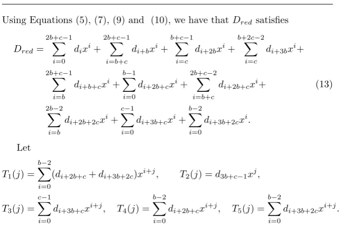
Using Equations (5), (7), (9) and (10), we have thatDredsatisfies
Dred=
2b+c−1 X
i=0
dixi+ 2b+c−1
X
i=b+c
di+bxi+ b+c−1
X
i=c
di+2bxi+ b+2c−2
X
i=c
di+3bxi+
2b+c−1 X
i=b
di+b+cxi+ b−1 X
i=0
di+2b+cxi+ 2b+c−2
X
i=b+c
di+2b+cxi+
2b−2 X
i=b
di+2b+2cxi+ c−1 X
i=0
di+3b+cxi+ b−2 X
i=0
di+3b+2cxi.
(13)
Let
T1(j) = b−2 X
i=0
(di+2b+c+di+3b+2c)xi+j, T2(j) =d3b+c−1xj,
T3(j) = c−1 X
i=0
di+3b+cxi+j, T4(j) = b−2 X
i=0
di+2b+cxi+j, T5(j) = b−2 X
i=0
di+3b+2cxi+j.
Again, a careful analysis of Equation (13) shows thatT1,T2 andT3 are used more than once. Thus, we can rewrite Equation (13) forDredas
Dred=B0+T1(0) +T1(b) +T1(b+c)+
T2(b−1) +T2(b+c−1) +T2(2b−1) +T2(2b+c−1)+ T3(0) +T3(c) +T3(2b) +T4(c) +T5(2c).
(14)
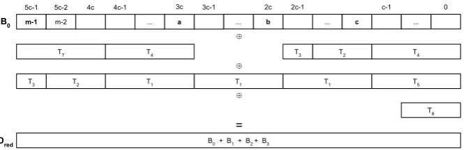
Figure 3 depicts these operations. Using Equation (14) and Figure 3, we have Algorithm 2. For code efficiency reasons, in contrast to Algorithm 1, in Algo-rithm 2 we separate the last line before the equality in Figure 3. The additions of this last line are done in lines 17 to 20 of Algorithm 2. As a consequence, lines 3 to 16 of Algorithm 2 include only the additions per column from 0 to 2b+c−1 of the first three lines in Figure 3.
m-1 ...
B0 + B1 + B2 + B3
B0
Dred
T2 T2
b+c
a
... ... ... ...
m-2 ... b c
T2 T1 T2 T1
T1 T3 T3 T3 T4 T5 b-2 0 b 2b-2 b+c 2b+c-2 2b+c-1 2b+c-2 0 c-1 c 2c-1 2b 2b+c-1 c b+c-2 2c b+2c-2 0 c-1 b-1 2c b+c-1 2b-1 2b ⊕ ⊕ ⊕ =
Fig. 3 Representation of the reduction byf(x) =x2b+c+xb+c+xb+xc+ 1, c >1.
The time delay is 3TX; after removal of redundancies and not counting repeated terms, we obtain that the numberN⊕ of XORs is
Algorithm 2ComputingDred forf(x) =x2b+c+xb+c+xb+xc+ 1.
input :D0=d[2b+c−1. . .0] bits vector of length 2b+c output:Dred
fori←0tob−2do
T1[i]←d[i+ 2b+ 1]⊕d[i+ 3b+ 2c]; .Definition ofT1 end
fori←0toc−1do
Dred[i]←d[i]⊕T1[i]; .Columns 0 toc−1 of the first three lines of Fig. 3 end
fori←ctob−2do
Dred[i]←d[i]⊕T1[i]⊕d[i+ 2b] end
Dred[b−1]←d[b−1]⊕d[3b+c−1]⊕d[3b−1] fori←btob+c−2do
Dred[i]←d[i]⊕T1[i−b]⊕d[i+ 2b] end
Dred[b+c−1]←d[b+c−1]⊕d[3b+c−1]⊕T1[c−1] fori←b+cto2b−2do Dred[i]←d[i]⊕T1[i−b]⊕T1[i−b−c]
end
Dred[2b−1]←d[2b−1]⊕d[3b+c−1]⊕T1[b−c−1] fori←2bto2b+c−2do Dred[i]←d[i]⊕T1[i−b−c]⊕d[i+b+c]
end
Dred[2b+c−1]←d[2b+c−1]⊕d[3b+c−1]⊕d[3b−1] fori←0toc−1do
Dred[i]←Dred[i]⊕d[i+ 3b+c]; .Columns 0 toc−1 of the 4thline of Fig. 3 end
fori←ctob+ 2c−2do
Dred[i]←Dred[i]⊕d[i+ 3b]; .Colsctob+ 2c−2 of the 4thline of Fig. 3 end
returnDred
Theorem 2 Algorithm 2 correctly gives the reduction of a polynomial of de-gree at most2m−2 over F2 by f(x) = x2b+c+xb+c+xb+xc+ 1involving N⊕ = 3m−2 = 6b+ 3c−2 number of XORs operations and a time delay of 3TX.
5.1 Almost equally spaced pentanomials: the special caseb= 2c
Consider the special case b = 2c. In this case we obtain the almost equally spaced polynomials f(x) = x5c+x3c+x2c+xc+ 1. Our previous analysis when applied to these polynomials entails
Dred=
5c−1 X
i=0 dixi+
5c−1 X
i=3c
di+2cxi+ 3c−1
X
i=c
di+4cxi+ 4c−2
X
i=c
di+6cxi+ 5c−1
X
i=2c
di+3cxi+
2c−1 X
i=0
di+5cxi+ 5c−2
X
i=3c
di+5cxi+ 4c−2
X
i=2c
di+6cxi+ c−1 X
i=0
di+7cxi+ 2c−2
X
i=0
di+8cxi.
Let
T1(j) = 2c−2
X
i=c
(di+5c+di+4c)xi+j, T2(j) = 2c−2
X
i=c
(di+8c+di+6c)xi+j,
T3(j) =d8c−1xj, T4(j) = c−1 X
i=0
di+8cxi+j, T5(j) = c−1 X
i=0
di+5cxi+j,
T6(j) = c−2 X
i=0
di+7cxi+j, T7(j) = 5c−1
X
i=4c
di+2cxi+j.
In the computation of Dred, T1, T2,T3 andT4 are used more than once. Figure 4 shows, graphically, these operations. After removal of redundancies, the numberN⊕ of XORs is N⊕= 12c−1 =
12
5 m−1.This number of XORs is close to 2.4m providing a saving of about 20% with respect to the other pentanomials in our family. Irreducible pentanomials of this form are rare but they do exist, for example, for degrees 5, 155 and 4805. We observe that the extension 155 is used in [1].
m-1 ...
B0 + B1 + B2 + B3
B0
Dred
3c
a ...
...
m-2 b c
5c-1 5c-2 4c 4c-1 3c-1 2c 2c-1 c-1 0
T4
T2
T3
T5
T1
T1
T1
T2
T3
T4
...
T6
T7
⊕
⊕
⊕
=
Fig. 4 Representation of the reduction by the almost equally spaced pentanomials (the special caseb= 2c).
Using Equation (15) and Figure 4, we naturally have Algorithm 3.
6 Multiplier inF2[x], complexity analysis and comparison
So far, we have focused on the second step of the algorithm, that is, on the reduction part. For the first step, the multiplication part, we simply use a standard Karatsuba recursive algorithm implementation; see Algorithm 4.
Recursivity in hardware can be an issue; see [24] and [13], for example, for efficient hardware implementations of polynomial multiplication in finite fields using Karatsuba’s type algorithms.
Algorithm 3ComputingDred forf(x) =x5c+x3c+x2c+xc+ 1.
input :D0=d[5c−1. . .0] bits vector of length 5c output:Dred
fori←0toc−2do
T1[i]←d[i+ 6c]⊕d[i+ 5c] .Definition ofT1 end
fori←0toc−2do
T2[i]←d[i+ 9c]⊕d[i+ 7c] .Definition ofT2 end
fori←0toc−2do
Dred[i]←d[i]⊕d[i+ 8c]⊕d[i+ 5c]⊕d[i+ 7c] end
Dred[c−1]←d[c−1]⊕d[9c−1]⊕d[6c−1] fori←cto2c−2do
Dred[i]←d[i]⊕T1[i−c]⊕T2[i−c] end
Dred[2c−1]←d[2c−1]⊕d[8c−1]⊕T1[c−1] fori←2cto3c−1do
Dred[i]←d[i]⊕T1[i−2c] end
fori←3cto4c−1do
Dred[i]←d[i]⊕T1[i−3c]⊕d[i+ 5c] end
fori←4cto5c−2do
Dred[i]←d[i]⊕T2[i−4c]⊕d[i+ 2c] end
Dred[5c−1]←d[5c−1]⊕d[8c−1]⊕d[7c−1] returnDred
Algorithm 4Karatsuba Algorithm forF2m
input :A(x) =Pm−1
i=0 aixiandB(x) =Pmi=0−1bixi output:C(x) =A(x)B(x) =P2i=0m−2cixi
FunctionKaratsuba(A,B):
m←maxDegree(A, B) .compute the larger degree between polynomialsAandB ifm = 0 then
return(A&B) .& is a bitwise AND operator
end
m2 =f loor(m/2) .splitAandB
higha,lowa←split(A, m2)
highb,lowb←split(B, m2)
d0←Karatsuba(lowa,lowb) .recursive call of Karatsuba
d1←Karatsuba((lowa⊕higha),(lowb⊕highb)) .recursive call of Karatsuba
d2←Karatsuba(higha,highb) .recursive call of Karatsuba
c←d2xm⊕(d1⊕d2⊕d0)xm2⊕d0 returnc
End Function
0 100 200 300 400 500 600 700 800 900 1,000 3.5
4 4.5 5 5.5 6
Deg
C
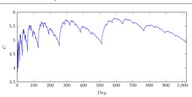
Fig. 5 Karatsuba constant for degrees up to 1024.
We chose the Karatsuba multiplier since our goal is to minimize the area, i.e. to minimize the number of gates AND and XOR. A summary of our re-sults compared with related works is given in Tables 1 and 2. Table 1 presents comparison costs among multipliers that perform two steps for the multipli-cation, that is, they execute a multiplication followed by a reduction. The table shows the multiplication algorithm used in each case. Table 2 gives a comparison among the state-of-the-art bit multipliers in the literature. The main target for us is [18] since it presents the smallest area in the literature. However, Type 3 polynomials are also considered; this is another practically relevant family of polynomials. With respect to Karatsuba variants, Table 3 of survey [4] shows asymptotic complexities of several Karatsuba multiplication algorithms without reduction.
For each entry in Table 1, we give the multiplication algorithm and the amount of gates AND, XOR as well its delay. We point that for [19] and [25], their multipliers are general for any pentanomial with a ≤ m
2 instead of for a specific family such as [20]. In the case of our family, in addition to the number of XORs for the reduction, we include the cost for the multiplication due to the recursive Karatsuba implementation multiplier, that is, the XOR count is formed by the sum of the XORs of the Karatsuba multiplier and the ones of the reduction part. In our implementation, the constant of Karatsuba is strictly less than 6; see Figure 5 for degrees up to 1024. As can be seen, for degrees powers of 2 minus 1 (2k −1, k ≥1), the constant achieves local minimum. For the number of AND gates, we provide an interval. The actual number of AND gates depends on the value ofm; it only reaches a maximum whenm= 2k−1, for k≥1.
Table 1 Two steps multipliers cost comparison for different family of pentanomials.
xm+xa+xb+xc+ 1 [25, 20], Multiplication algorithm: Schoolbook.
Costs #AND #XOR Delay
Reduction 0 4(m−1) 3TX
Multiplication m2 (m−1)2 T
A+ (dlog2me)TX Multiplier m2 m2+ 2m−3 T
A+ (3 +dlog2me)TX TypeI-xm+xn+1+xn+x+ 1 [20], Multiplication algorithm: Mastrovito-like Multiplier.
Costs #AND #XOR Delay
Reduction 0 3m+ 2n−1 3TX
Multiplication m2 m2−2m+ 1 T
A+ (dlog2me)TX Multiplier m2 m2+m+ 2n T
A+ (3 +dlog2me)TX TypeI-xm+xn+1+xn+x+ 1 [19], Multiplication algorithm: Mastrovito-like Multiplier.
Costs #AND #XOR Delay
Reduction 0 3m−2 3TX
Multiplication m2 m2−2m+ 1 T
A+ (dlog2(m−1)e)TX Multiplier m2 m2+m† T
A+ (3 +dlog2(m−1)e)TX TypeII-xm+xn+2+xn+1+xn+ 1 [20], Multiplication algorithm: Dual basis.
Costs #AND #XOR Delay
Reduction 0 3m− d(m−2)/2e+ 3n−4 3TX Multiplication m2 m2−m T
A+ (dlog2me)TX Multiplier m2 m2+ 2m− d(m−2)/2e+ 3n−4 T
A+ (3 +dlog2me)TX
xm+xa+xb+xc+ 1, c >1 [19], Multiplication algorithm: Mastrovito-like Multiplier.
Costs #AND #XOR Delay
Reduction 0 4m−4 4TX
Multiplication m2 m2−2m+ 1 T
A+ (dlog2(m−1)e)TX Multiplier m2 m2+ 2m−3 T
A+ (4 +dlog2(m−1)e)TX Ours -x2b+c+xb+c+xb+xc+ 1, Multiplication algorithm: Karatsuba.
Costs #AND #XOR Delay
Reduction 0 3m−2 3TX
Multiplication (3blog2mc,3blog2mc+1] <6mlog23 TA+ 3dlog2(m−1)eTX Multiplier (3blog2mc,3blog2mc+1] <6mlog23+ 3m−2 TA+ 3(dlog2(m−1)e+ 1)TX
Ours -x5c+x3c+x2c+xc+ 1, Multiplication algorithm: Karatsuba.
Costs #AND #XOR Delay
Reduction 0 (12/5)m−1 3TX Multiplication (3blog2mc,3blog2mc+1] <6mlog23 TA+ 3dlog2(m−1)eTX Multiplier (3blog2mc,3blog2mc+1] <6mlog23+ (12/5)m−1 TA+ 3(dlog2(m−1)e+ 1)TX
†There is an additional XOR to reduce the time delay; see [19, page 955].
we separate these two parts and use Karatsuba for the multiplier followed by our reduction algorithm.
Table 2 Space and time complexities of state-of-the-art bit multipliers.
Type # XOR # AND Delay
Type 1 xm+xb+1+xb+x+ 1, 1< b≤m
2−1
[18] bis odd 3m
2+ 24m+ 8b+ 21 4
3m2+ 2m−1
4 TA+ (3 +dlog2(m+ 1)e)Tx
[18] bis even 3m
2+ 24m+ 8b+ 17 4
3m2+ 2m−1
4 TA+ (3 +dlog2(m+ 1)e)Tx Type 2 xm+xc+2+xc+1+xc+ 1
[18] cis odd,c≤3 8(m−7)
3m2+ 24m+ 14c+ 35 4
3m2+ 2m−1
4 TA+ (3 +dlog(m+ 1)e)Tx [18] cis even,c≤m
2−1
3m2+ 24m+ 14c+ 45 4
3m2+ 2m−1
4 TA+ (3 +dlog(m+ 1)e)Tx [20] c >1 m2+ 2m
− d(m−2)/2e+ 3n−4 m2 T
A+ (3 +dlog(m−1)e)Tx
[20] c= 1 m2+m
−2 m2 T
A+ (3 +dlog2(m−1)e)Tx
Type 3 xm+xm−c+xm−2c+xm−3c+ 1
[19] m−1 4 ≤c≤
m−1
3 m
2+m−c−1 m2 T
A+ (3 +dlog2(m−1)e)Tx
[19] m−1 5 ≤c <
m−1
4 m
2+ 2m−5c−2 m2 T
A+ (3 +dlog2(m−1)e)Tx
[19] m−1 8 ≤c <
m−1
5 m
2+m−2 m2 T
A+ (3 +dlog2(m−1)e+ 1)Tx
Ours x2b+c+xb+c+xb+xc+ 1
Ours c≥1,b6= 2c <6mlog23+ 3m−2 (3blog2mc,3blog2mc+1] T
A+ 3(dlog2(m−1)e)Tx
Ours c≥1,b= 2c <6mlog23+12
5m−1 (3b
log2mc,3blog2mc+1] T
The costs for using our pentanomials for degrees proposed by NIST can be found in Table 3. The amount of XOR and AND gates are the exact value obtained from Table 1. The delay costs can be separated inTAandTX, delay for AND gates and XOR gates, respectively. The delay for AND gates is due to only 1 AND gate at the lowest level of the Karatsuba recursion. The delay for the XOR gates in the Karatsuba multiplier is 3dlog2(m−1)esince there are 3 delay XORs per level of the Karatsuba recursion. For the reduction part, we only have 3 delay XORs. Hence, the total number of XOR delays is 3dlog2(m−1)e+ 3.
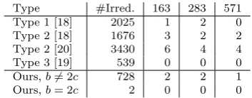
Table 4 shows the number of irreducible pentanomials of degrees 163, 283 and 571 for the families considered since those are NIST degrees where pen-tanomials have been recommended [16]. Analyzing the table, we have that family Type 1 has the most irreducible pentanomials, but few of them have degrees recommended by NIST [16]. The first family of Type 2, proposed in [18], has restrictions in the range ofc; this family presents the highest number of representatives with NIST degrees of interest. The second family of Type 2, proposed in [20], has no restrictions forc; this family presents the largest num-ber of irreducible polynomials. Type 3 is the special case from [19]. Our family forb6= 2chas less irreducible polynomials and it has no irreducible polynomi-als with degrees 163, 283 and 571. In the other side, whenb 6= 2cour family has 730 polynomials of degrees up to 1024 and it presents 5 pentanomials of NIST degrees.
In the following we comment on the density of irreducible pentanomials in our family. Table 5 lists all irreducible pentanomials of our family for degrees up to 1024;N⊕is the number of XORs required for the reduction. We leave as an open problem to mathematically characterize under which conditions our pentanomials are irreducible.
Table 3 Costs for fixed degree pentanomials proposed by NIST.
Degree XORs ANDs Delay
Karatsuba Reduction Total
163 17,944 487 18,431 4,419 TA+ 27TX
283 43,162 847 44,009 10,305 TA+ 30TX
571 132,280 1,711 133,991 31,203 TA+ 33TX
Table 4 Number of irreducible pentanomials for NIST degrees.
Type #Irred. 163 283 571
Type 1 [18] 2025 1 2 0
Type 2 [18] 1676 3 2 2
Type 2 [20] 3430 6 4 4
Type 3 [19] 539 0 0 0
Ours,b6= 2c 728 2 2 1
Table 5: Our family of irreducible pentanomials and their number of XORs (b, c, N⊕), 2b6=c.
7 Conclusions
In this paper, we present a new class of pentanomials over F2, defined by x2b+c+xb+c+xb+xc+ 1. We give the exact number of XORs in the reduction process; we note that in the reduction process no ANDs are required.
It is interesting to point out that even though the cases c= 1 and c >1, as shown in Figures 2 and 3, are quite different, the final result in terms of number of XORs is the same. We also consider a special case when b = 2c
where further reductions are possible.
There are irreducible pentanomials of this shape for several degree exten-sions of practical interest. We provide a detailed analysis of the space and time complexity involved in the reduction using the pentanomials in our family. For the multiplication process, we simply use the standard Karatsuba algorithm.
The proved complexity analysis of the multiplier and reduction considering the family proposed in this paper, as well as our analysis suggests that these pentanomials are as good as or possibly better to the ones already proposed. We leave for future work to produce a one-step algorithm using our pen-tanomials, that is, a multiplier that performs multiplication and reduction in a single step using our family of polynomials, as well as a detailed study of the delay obtained using this algorithm.
References
1. G.B. Agnew, R.C. Mullin, and S.A. Vanstone. An implementation of elliptic curve cryp-tosystems overF2155. IEEE Journal on Selected Areas in Communications, 11(5):804-813, 1993
2. D. J. Bernstein and P. Schwabe. Neon crypto. In International Workshop on Crypto-graphic Hardware and Embedded Systems, pages 320339. Springer, 2012.
3. A. Cilardo. Fast parallelGF(2m) polynomial multiplication for all degrees. IEEE
Trans-actions on Computers, 62(5):929-943, 2013.
4. H. Fan and M.A. Hasan. A survey of some recent bit-parallelGF(2n) multipliers. Finite
Fields and Their Applications, 32:5-43, 2015.
5. J. Fan, X. Guo, E. De Mulder, P. Schaumont, B. Preneel, and I. Verbauwhede. State-of-the-art of secure ECC implementations: a survey on known side-channel attacks and countermeasures. In Hardware-Oriented Security and Trust (HOST), 2010 IEEE In-ternational Symposium on, pages 76-87. IEEE, 2010.
6. A. Halbutogullari and C.K. Ko¸c. Mastrovito multiplier for general irreducible polyno-mials. IEEE Transactions on Computers, 49:503-518, 2000.
7. M.A. Hasan, M. Wang, and V.K. Bhargava. Modular construction of low complexity parallel multipliers for a class of finite fieldsGF(2m). IEEE Transactions on Computers,
41:962-971, 1992.
8. J.L. Ima˜na. High-speed polynomial basis multipliers over GF(2m) for special
pen-tanomials. IEEE Transactions on Circuits and Systems I: Regular Papers, 63(1):58-69, 2016.
9. J.L. Ima˜na, R. Hermida, and F. Tirado. Low complexity bit-parallel multipliers based on a class of irreducible pentanomials. IEEE Transactions on Very Large Scale Integration (VLSI) Systems, 14(12):1388-1393, 2006.
10. J.L. Ima˜na, R. Hermida, and F. Tirado. Low complexity bit-parallel polynomial basis multipliers over binary fields for special irreducible pentanomials. Integration, the VLSI Journal, 46(2):197-210, 2013.
12. R. Lidl and H. Niederreiter. Finite Fields. Cambridge University Press, Cambridge, 1997.
13. M. Machhout, M. Zeghid, B. Bouallegue, and R. Tourki. Efficient hardware architecture of recursive Karatsuba-Ofman multiplier. In Design and Technology of Integrated Sys-tems in Nanoscale Era, 2008. DTIS 2008. 3rd International Conference on, pages 1-6. IEEE, 2008.
14. G.L. Mullen and D. Panario. Handbook of Finite Fields. CRC Press, 2013.
15. C. Negre and J. Robert. Impact of optimized field operations AB, AC and AB+CD in scalar multiplication over binary elliptic curve. In International Conference on Cryptol-ogy in Africa, pages 279-296. Springer, 2013.
16. NIST. Digital signature standard. Report P-41, National Institute of Standards and Technology (NIST), 2000.
17. T. Oliveira, J. L´opez, and F. Rodr´ıguez-Henr´ıquez. Software implementation of Koblitz curves over quadratic fields. In International Conference on Cryptographic Hardware and Embedded Systems, pages 259-279. Springer, 2016.
18. S.-M. Park, K.-Y. Chang, D. Hong, and C. Seo. New efficient bit-parallel polynomial basis multiplier for special pentanomials. Integration, the VLSI Journal, 47(1):130-139, 2014.
19. A. Reyhani-Masoleh and M.A. Hasan. Low complexity bit parallel architectures for poly-nomial basis multiplication overGF(2m). IEEE Transactions on Computers, 53:945-959, 2004.
20. F. Rodr´ıguez-Henr´ıquez and C.K. Ko¸c. Parallel multipliers based on special irreducible pentanomials. IEEE Transactions on Computers, 52:1535-1542, 2003.
21. M. Scott. Optimal irreducible polynomials forGF(2m) arithmetic. IACR Cryptology
ePrint Archive, 2007:192, 2007.
22. B. Sunar and C.K. Ko¸c. Mastrovito multiplier for all trinomials. IEEE Transactions on Computers, 48:522-527, 1999.
23. T. Unterluggauer and E. Wenger. Efficient pairings and ECC for embedded systems. In International Workshop on Cryptographic Hardware and Embedded Systems, pages 298-315. Springer, 2014.
24. J. von zur Gathen and J. Shokrollahi. Efficient FPGA-based Karatsuba multipliers for polynomials overF2. In International Workshop on Selected Areas in Cryptography,
pages 359-369. Springer, 2005.
25. H. Wu. Low complexity bit-parallel finite field arithmetic using polynomial basis. Cryp-tographic Hardware and Embedded Systems, pages 280-291. Springer, 1999.
26. H. Wu. Bit-parallel finite field multiplier and squarer using polynomial basis. IEEE Transactions on Computers, 51(7):750-758, 2002.
27. H. Wu. Bit-parallel polynomial basis multiplier for new classes of finite fields. IEEE Transactions on Computers, 57:1023-1031, 2008.