Saber: Module-LWR based key exchange,
CPA-secure encryption and CCA-secure KEM
Jan-Pieter D’Anvers, Angshuman Karmakar Sujoy Sinha Roy, and Frederik Vercauteren
imec-COSIC, KU Leuven
Kasteelpark Arenberg 10, Bus 2452, B-3001 Leuven-Heverlee, Belgium [email protected]
Abstract In this paper, we introduce Saber, a package of cryptographic primitives whose security relies on the hardness of the Module Learning With Rounding problem (Mod-LWR). We first describe a secure Diffie-Hellman type key exchange protocol, which is then transformed into an IND-CPA encryption scheme and finally into an IND-CCA secure key encapsulation mechanism using a post-quantum version of the Fujisaki-Okamoto transform. The design goals of this package were simplicity, efficiency and flexibility resulting in the following choices: all integer moduli are powers of 2 avoiding modular reduction and rejection sam-pling entirely; the use of LWR halves the amount of randomness re-quired compared to LWE-based schemes and reduces bandwidth; the module structure provides flexibility by reusing one core component for multiple security levels. A constant-time AVX2 optimized software im-plementation of the KEM with parameters providing more than 128 bits of post-quantum security, requires only 101K, 125K and 129K cycles for key generation, encapsulation and decapsulation respectively on a Dell laptop with an Intel i7-Haswell processor.
1
Introduction
and ’a New Hope’ by using modules. Concurrently to our work, Jin et al. de-scribed a generic key exchange for Ring-LWE, Mod-LWE, LWE and LWR in [33], and Baan et al. [8] described a LWR, Ring-LWR key exchange.
In this paper, we introduce Saber, a suite of cryptographic primitives based on the Mod-LWR problem. The choices we made for the underlying hard prob-lem and also the actual parameters of the scheme were motivated by three design principles: simplicity of the scheme and its implementation, efficiency and flexi-bility:
– Learning with Rounding (LWR) [10]: schemes based on (variants of) LWE require sampling from noise distributions, which needs randomness. Further-more, the noise is included in public keys and ciphertexts resulting in higher bandwidth. LWR based schemes naturally reduce the bandwidth while avoid-ing additional randomness for the noise since it is deterministically obtained.
– Choice of moduli: we choose all integer moduli in the scheme to be powers of 2. This eliminates the need for explicit modular reduction and complicated sampling routines such as rejection sampling. We also prove that using pow-ers of two, the keys are unbiased and that there is no need for steps such as uplifting and randomization or decoding of the exchanged information. These advantages contribute to the simplicity of our design, and facilitate constant time implementations. The main disadvantage of using such mod-uli is that it excludes the use of the number theoretic transform (NTT) to speed up polynomial multiplication. We propose the use of a combination of Toom-Cook and Karatsuba polynomial multiplication to mitigate this disadvantage.
– Modules [36,16]: the module versions of the problems (see Section 2) allow to interpolate between the original pure LWE/LWR problems and their ring versions, lowering computational complexity and bandwidth compared to LWE/LWR, while introducing protection against attacks on the ring struc-ture of Ring-LWE/LWR and flexibility to move to higher security levels without any need to change the underlying arithmetic.
A high-level constant-time software implementation of Saber is provided and has been placed in the public domain1 as part of the submission to the NIST competition. The implementation has been optimized using AVX2 instructions available in modern Intel processors and uses a combination of Toom-Cook and Karatsuba polynomial multiplication algorithms.
The remainder of the paper is organised as follows: in Section 2 we review the necessary background; we present a secure Diffie-Hellman type key exchange scheme in Section 3, a CPA secure encryption scheme in Section 4 and a CCA secure key encapsulation mechanism in Section 5. A security analysis of the hardness on the underlying mod-LWR problem is given in Section 6.1, based on which three parameter sets are chosen in Section 6.2. Finally, specific implemen-tation choices that speed up our protocols are discussed in Section 7 and our implementation results are compared with the state of the art in Section 8.
1
2
Preliminaries
2.1 Notation
We denote withZq the ring of integers modulo an integerqwith representants in
[0, q) and for an integerz, we denotezmodqthe reduction ofzin [0, q).Rqis the
quotient ringZq[X]/(Xn+ 1) withna fixed power of 2 (we only needn= 256).
For any ring R, Rl×k denotes the ring of l×k-matrices over R. For p| q, the
modpoperator is extended to (matrices over)Rqby applying it coefficient-wise.
Single polynomials are written without markup, vectors are bold lower case and matrices are denoted with bold upper case. U denotes the uniform distribution andβµis a centered binomial distribution with parameterµand corresponding
standard deviation σ = pµ/2. If χ is a probability distribution over a set S, then x ← χ denotes sampling x ∈ S according to χ. If χ is defined on Zq,
XXX ←χ(Rl×k
q ) denotes sampling the matrixXXX ∈Rql×k, where all coefficients of
the entries inXXX are sampled fromχ.
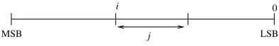
We use the part selection functionbits(x, i, j) withj ≤i to access j con-secutive bits of a positive integer x ending at the i-th index (assuming least significant bit in the 0-th index), producing an integer in Z2j; i.e., written in standard C code the function returns (x(i−j))&(2j −1), where is the
right-shift operator. This is explained in Fig. 1.The part selection function is extended to polynomials and matrices by applying it coefficient-wise. Finally let bedenote rounding to the nearest integer, which can be extended to polynomials and matrices coefficient-wise.
i 0
LSB
MSB j
Figure 1: Thebits(x, i, j) operator.
2.2 Cryptographic definitions
Let KE be a Diffie-Hellman type key exchange protocol between two parties as illustrated in Protocol 1. KE is called (1−δ)-correct if after execution of the protocolP r[k0 =k]>1−δ, where the probability is computed over the random coins used in Protocol 1. KE is called IND-RND secure if it is hard for an adversary to distinguish the real shared secret from random. More formally, we define the advantage of an adversary in distinguishing the keykfrom a uniformly random key ˆk← U(K) as follows:
Advind-rndKE (A) = P r
A(P,A,B, k) = 1 −P r
Public parameters P
Alice Bob
Choose secreta
ComputeAas function ofPanda A
-Choose secretb
ComputeBas function ofPandb
B
k= Derive key fromP, a,B k0= Derive key fromP, b,A
Protocol 1: Diffie-Hellman type key exchange protocol
Enctakes a public keypk and a messagem∈ Mto produce a ciphertextc∈ C, andDectakes the secret keysktogether with ciphertextc to output a message m0 ∈ M or the symbol ⊥to denote rejection. The PKE is said to be (1−δ )-correct if P r[Dec(sk,Enc(pk, m)) = m]>1−δ, where the probability is taken over (pk, sk) ← KeyGen and the random coins of Enc. We use the notion of indistinguishability under chosen plaintext attacks (IND-CPA) and define the advantage of an adversary A by:
Advind-cpaenc (A) = P r
b0 =b:
(pk, sk)←KeyGen();
(m1, m2)←AEnc(pk); b← U({0,1}); c←Enc(pk, mb); b0 ←AEnc(pk, c);
− 1 2 .
The weaker notion of one-wayness under chosen plaintext attacks (OW-CPA) is defined as:
Advow-cpaenc (A) = P r m 0=m:
(pk, sk)←KeyGen(); m← M; c←Enc(pk, m);
m0←AEnc(pk, c); − 1 2 .
A key-encapsulation mechanism KEM = (KeyGen,Encaps,Decaps) is a triple of probabilistic algorithms, where KeyGenreturns a secret key sk and a public keypk, whereEncaps takes a public keypk and produces a ciphertextc and a key k ∈ K, and where Decaps takes the secret key sk, the public key pk and ciphertextcto return a keyk∈ Kor the symbol⊥to denote rejection. The KEM is said to be (1−δ)-correct ifP r[Decaps(sk, c) =k: (c, k)←Encaps(pk)]>1−δ, where the probability is taken over (pk, sk)←KeyGenand the random coins of
Encaps. We use the notion of indistinguishability under chosen ciphertext attacks (IND-CCA) to define the advantage of an adversaryAby:
Advind-ccaKEM (A) = P r
b0=b:
(pk, sk)←KeyGen(); b← U({0,1}); (c, d, k0)←Encaps(pk); k1← K; b0 ←ADecaps(pk, c, d, kb);
− 1 2 .
The advantage of an adversary A in distinguishing a pseudorandom generator
defined as follows:
Advprg
gen()(A) =
P r
b0 = 1 : seedAAA← U({0,1} 256) A
A
A←gen(seedAAA)∈Rql×l;b0=A(AAA);
.
−P r
b0 = 1 :AAA← U(Rm×l
q );b0 =A(AAA);
(1)
2.3 LWE, LWR and Mod-LWR problems
The learning with errors (LWE) problem was introduced by Regev [41] and its decisional version states that it is hard to distinguish uniform random samples (aaa, u)← U(Zlq×1×Zq) from LWE-samples of the form
a
aa, b=aaaTsss+e ∈ Zlq×1×Zq, (2)
where the secret vector sss ← βµ(Zql×1) is fixed for all samples, aaa ← U(Zlq×1)
and e←βµ(Zq) is a small error. A module version of LWE, called Mod-LWE,
was analyzed by Langlois and Stehl´e [36] and essentially replaces the ringZq in
the above samples by a quotient ring of the form Rq with corresponding error
distributionβµ(Rql×1). The rank of the module island the dimension of the ring
Rq isn. The casel= 1 corresponds to the ring-LWE problem introduced in [37].
The LWR problem was introduced by Banerjee et al. [10] and is a derandom-ized version of the LWE problem. In contrast to the LWE problem, the “noise” in the LWR problem is generated deterministically by scaling and rounding co-efficients moduloqto modulop(withp < q). In detail, an LWR sample is given by
aaa, b=jp q(aaa
Tsss)m ∈
Zlq×1×Zp (3)
for a fixedsss←βµ(Zql×1) and uniform randomaaa← U(Zlq×1). The decisional LWR
problem states that is it hard to distinguish samples from the LWR distribution from that of the uniform distribution. A reduction from the LWE problem to the LWR problem was given by Banerjee et al. [10], and further improved by Alwen et al. [6], Bogdanov et al. [15] and, Alperin-Sheriff and Daniel Apon [5].
The security of our protocol relies on the hardness of the module version of LWR (Mod-LWR), which is a straightforward generalization of Mod-LWE. A Mod-LWR sample is given by
a
aa, b=jp q(aaa
Tsss)m ∈ Rl×1
q ×Rp (4)
where the secretsss←βµ(Rql×1) is fixed for all samples andaaa← U(Rlq×1).
m,k,µ,qandpare positive integers withq > p:
AdvMod-LWRm,l,µ,q,p (A) =
P r
b0= 1 :AAA← U(R
m×l
q ); sss←βµ(Rlq×1);
b0=A(AAA,b(p/q)AAAssse);
−P r
b0= 1 :AAA← U(R
m×l
q ); uuu← U(Rlp×1);
b0 =A(AAA, uuu);
. (5)
3
Key Exchange
In Protocol 2 we describe a Diffie-Hellman type key exchange scheme Saber.KE based on the hardness of Mod-LWR problem. Unlike the Diffie-Hellman key exchange [23], in our scheme the two communicating parties sometimes fail to agree on the same key. As in previous works [24,40,12], we can make this failure probability negligibly small by sending some additional reconciliation datac.
Alice Bob
1 seedAAA← U({0,1}256)
2 AAA←gen(seedAAA)∈Rlq×l
3 sss←βµ(Rlq×1) sss0←βµ(Rlq×1)
4 bbb=bits(AAAsss+hhh, q, p)∈Rpl×1 bbb,seed-AAA AAA←gen(seedAAA)∈Rlq×l
5 bbb0=bits(AAATsss0+hhh, q, p)∈Rlp×1
6 v0=bbbTbits(sss0, p, p) +h1∈Rp
7 v=bbb0Tbits(sss, p, p) +h1∈Rp
bbb0, c c=bits(v0
, p−1, t)∈Rt
8 k=bits(v−2p−t−1c+h
2, p,1) k0=bits(v0, p,1)
9 keyAlice=kdf(k) keyBob=kdf(k0)
Protocol 2: Saber.KE key exchange
All moduli involved in the scheme are chosen to be powers of 2, in particular we chooseq= 2q,p= 2pandt= 2t with
q > p>(t+1), so we have 2t|p|q.
In practice, our main parameter set will correspond to the caseq = 13,p= 10
andt= 3. The secret vectorssssandsss0 are sampled fromβµ(Rql×1), withµ < p,
while the matrixAAA ∈ Rlq×l is sampled using a pseudorandom generator gen()
initialized with seedA. The session key is obtained by feeding the common secret
k=k0∈R
2 into a key derivation functionkdf(). The algorithm also uses three constants: a constant vectorhhh∈Rl×1
q consisting of polynomials all coefficients
of which are set to the constant 2q−p−1, a constant polynomialh
1 ∈Rq with
all coefficients equal to 2q−p−1, and a constant polynomial h
2 ∈ Rq with all
Note that the operationsbits(sss, p, p) in line6andbits(sss0, p, p) in line7
simply mean we are consideringsssmodpandsss000modpas elements in Rp which
is well defined since p|q.
Correctness: Using Saber.KE two communicating parties agree on a com-mon random key with overwhelming probability. A tight bound on the failure probability can be obtained using following observations from Bos et al. [17]: the reconciliation between two integer values vi, vi0 ∈ Zp is correct if the distance
betweenviandvi0 is smaller thanp/4(1−1/t), and fails if the distance is bigger
thanp/4(1 + 1/t). In between these values, the probability of success decreases linearly from 1 to 0. Consequently, a tight bound on the failure probability given the distribution of∆vi=v0i−vi can be calculated by adding to∆vi a discrete
uniformly distributed error er∈Zp with range [−p/4t, p/4t]. The success
prob-ability of the reconciliation betweenvi andv0i then equalsP r[|∆vi+er|< p/4].
Using the above observation we can estimate a bound on the error probability:
Theorem 1. LetAAA be a matrix in Rlq×l andsss, sss0 two vectors in Rlq×1 sampled as in Protocol 2. Define eee andeee0 as the rounding errors introduced by scaling and roundingAAAsssandAAATsss0, i.e.
bits(AAAsss+h, hh q, p) =pqAsAAss+eeeandbits(AAATsss0+
hhh, q, p) = pqAAATsss0+eee000. Let er∈ Rq be a polynomial with uniformly distributed coefficients with range[−p/4t, p/4t]. If we set
δ=P r[||(sss0Teee−eee0Tsss+er) modp||∞> p/4]
then after executing the Saber.KE protocol, both communicating parties agree on an-bit key with probability1−δ.
Proof. The polynomials v0 and v calculated by Bob and Alice respectively in Protocol 2 are given as:v0 = (pqsss0TAAAsss+h
1+sss0Teee modp) andv= (pqsss
0TAAAsss+h
1+ eee0Tsss modp). Here, the coefficients ofeee, eee0 are the rounding errors and so are in
(−1/2,1/2]. It can be easily seen that the values calculated by the communicating parties differ by ∆v=||(sss0Teee−eee0Tsss) mod p||. Therefore, Bob and Alice agree
on the same secret if ||∆v+er||∞ ≤ p4. Hence, for δ=P r[||(sss
0Teee−eee0Tsss+e r)
modp||∞> p/4] the Saber.KE protocol is (1−δ) correct.
Similar to Bos et al. [16], a tight upper bound on the value ofδis calculated using a Python script. To be able to practically compute the distribution of ∆v = v0 −v ∈ Rp, Bos et al. assume independence between the terms sss0Teee
and eee0Tsss, which is not necessarily the case. Analogous to Theorem 5.2 from Jin and Zhao [33], one could argue that they are independent if conditioned on sss0TAAAsss ≡ a modq/p, where a ∈ R
q/p. The recommended parameter set
described in Section 6.2 yieldsδ <2−136.
Unbiased keys: Since our moduli are powers of 2 and as such non-prime, there exists (negligibly small) exceptional sets forsssandsss000such that the common key is biased. The intuition is that if all coefficients of the polynomials insssorsss000 are divisible by a high power of 2, the same property will hold forAAAsssorAAATsss000,
Theorem 2. Let Sbad denote the set of elements inRlq×1 for which none of the coefficientswsatisfiesgcd(w, q)|(q/p)and letSbad0 denote the set of elements in
Rl×1
q for which none of the coefficientsw satisfies gcd(w, p)|(p/2). Let sss, sss0 ←
βµ(Rlq×1)and letAAA← U(Rql×l)and determine kas follows:
1. bbb=bits(AAAsss+hhh, q, p) 2. k=bits(bbbT(sss0 modp) +h
1, p,1)
Forsss /∈ Sbad andsss0 ∈/ Sbad0 ,k is distributed uniformly forAAA ← U(Rql×l). This occurs with a probabilityP r[sss /∈Sbad]P r[sss0 ∈/ Sbad0 ].
Proof. Note that the multiplication of a uniformly distributed coefficient ofAAA, by a coefficientw ofsss, is uniformly distributed in itsp most significant bits if
gcd(w, q)|(q/p), which is equivalent to stating that bpw/qeis invertible inZp.
The distribution of the coefficients ofbbb =bits(AAAsss+hhh, q, p) is as follows:
since convolution of any distribution with a uniform distribution in Zp results
again in a uniform distribution inZp, we need only one term of the summation
step to be uniform in itspmost significant bits. Therefore, the coefficients ofbbb will be uniformly distributed ifsss /∈Sbad.
Finally note that the distribution ofk0 =bits(bbbT(sss0 modp) +h
1, p,1) is
uniform ifbbbhas a uniform distribution and ifsss0 ∈/ s0bad. As above, a multiplication of a uniformly distributed coefficient ofbbb, with a coefficientw0 ofsssis uniformly distributed in its most significant bit if gcd(w0, p)|(p/2). Therefore, k will be uniform if the coefficients ofbbb are uniformly distributed and ifsss0 ∈/ Sbad0 . The probability of a samplingsssandsss0 so that khas a uniform distribution is thus P r[sss /∈Sbad]P r[sss0∈/Sbad0 ].
Since in our settingsss, sss000 are sampled fromβµ(Rq), the coefficients are small
and thus the only sampleable vector in Sbad and S0bad is the all zero vector which occurs with probability 2−1436. In the rest of the paper, we assume that the secret vectors are not in the vector sets:sss /∈Sbad andsss0 ∈/ Sbad0 .
Security: The security of Saber.KE can be reduced to the decisional Mod-LWR problem as shown by the following theorem.
Theorem 3. For any adversary A, there exist three adversaries B0, B1 and B2
such that Advind-rndSaber.KE(A)6Advprggen()(B0) +Advmod-lwrl,l,µ,q,p(B1) +Advmod-lwrl+1,l,µ,q,p(B2),
if q/p6p/(2t).
Proof. The IND-RND security of our key exchange can be expressed as the probability that an adversary A can distinguish between k and a uniformly random key ˆk ← U(K), given the public information AAA,bbb,bbb0 and c. The proof
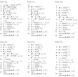
proceeds by a sequence of games Gi, where AdvGi(A) = |P r[SA,i]−1/2|, in which SA,i is the event that the adversary guesses correctly in game Gi. The
sequence of games is depicted in Figure 2.
GameG0:
1. seedAAA← U({0,1}256) 2. AAA←gen(seedAAA) 3. sss, sss0←βη(Rlq×1) 4. bbb=bits(
A
AA·sss+hhh, q, p) 5. bbb0=bits(
A
AAT·sss0+hhh, q, p) 6. v0=bbbT·bits(sss0,
p, p) +h1
7. c=bits(v0, p−1, t) 8. k0=bits(v0, p,1) 9. ˆk← U(R2) 10. u← U({0,1}) 11. ifu= 0:
return(AAA, bbb, bbb0, c, k0) 12. else:
return(AAA, bbb, bbb0, c,ˆk)
GameG1:
1.
2. AAA← U(Rlq×l) 3. sss, sss0←βη(Rlq×1) 4. bbb=bits(
A A
A·sss+hhh, q, p) 5. bbb0=bits(
A A
AT·sss0+hhh, q, p) 6. v0=bbbT·bits(sss0,
p, p) +h1
7. c=bits(v0, p−1, t) 8. k0=bits(v0, p,1) 9. ˆk← U(R2) 10. u← U({0,1}) 11. ifu= 0:
return(AAA, bbb, bbb0, c, k0) 12. else:
return(AAA, bbb, bbb0, c,ˆk)
GameG2:
1.
2. AAA← U(Rl×l q ) 3. sss0←βη(Rlq×1)
4. bbb← U(Rlp×1) 5. bbb0=bits(
A A
AT·sss0+hhh, q, p) 6. v0=bbbT·bits(sss0,
p, p) +h1
7. c=bits(v0, p−1, t) 8. k0=bits(v0, p,1) 9. ˆk← U(R2) 10. u← U({0,1}) 11. ifu= 0:
return(AAA, bbb, bbb0, c, k0) 12. else:
return(AAA, bbb, bbb0, c,ˆk)
GameG3: 2. AAA← U(Rlq×l) 3. sss0←βη(Rlq×1) 4. bbb← U(Rlp×1) 5. bbb0=bits(
A
AAT·sss0+hhh,
q, p) 6. v0=bbbT·bits(sss0,
p, p) +h1
7. c=bits(
v0, p−1,2p−q−1) 8. k0=bits(v0, p,1) 9. ˆk← U(R2) 10. u← U({0,1}) 11. ifu= 0:
return(AAA, bbb, bbb0, c, k0) 12. else:
return(AAA, bbb, bbb0, c,ˆk)
GameG4: 2. AAA← U(Rl×l
q ) 3. sss0←βη(Rlq×1)
4. bbb← U(Rlq×1) 5. bbb0=bits(
A A
AT·sss0+hhh,
q, p)
6. v0=bits(
b b
bT·sss0+h1, q, p) 7. c=bits(
v0, q−1, p−1) 8. k0=bits(v0, q,1) 9. ˆk← U(R2) 10. u← U({0,1}) 11. ifu= 0:
return(AAA, bbb, bbb0, c, k0) 12. else:
return(AAA, bbb, bbb0, c,ˆk)
GameG5:
2. AAA← U(Rl×l q ) 4. bbb← U(Rlq×1)
5. bbb0← U(Rlp×1)
6. v0← U(Rlp×1) 7. c=bits(
v0, p−1, p−1) 8. k0=bits(v0, p,1) 9. ˆk← U(R2) 10. u← U({0,1}) 11. ifu= 0:
return(AAA, bbb, bbb0, c, k0) 12. else:
return(AAA, bbb, bbb0, c,ˆk)
Figure 2: Sequence of games that are used in the proof of Theorem 3
two games, can also distinguish the matrix generated through the pseudorandom generator from a uniformly random matrix, and therefore|P r[SA,0]−P r[SA,1]|6 Advprggen()(B0).
During the second game G2, the vector bbb is generated uniformly random, so that (AAA, bbb) is a uniformly distributed sample, in contrast to the first game G1, where (AAA, bbb) forms a Mod-LWR sample. An adversary that can distinguish between gameG1 andG2 has also solved the decisional Mod-LWR problem on this sample, and therefore|P r[SA,1]−P r[SA,2]|6Advmod-lwrl,l,µ,q,p(B1).
In game G2, the number of bits dropped in the calculation of bbb0 and c is q−p andp−t−1 respectively, which is reduced toq−p in gameG3. If we compareG3 to G2, since (q−p)6(p−t−1), the number of dropped bits
Algorithm 1: Saber.KeyGen()
1 seedAAA← U({0,1}256)
2 AAA←gen(seedAAA)∈Rlq×l 3 sss←βµ(Rlq×1)
4 bbb=bits(AAAsss+h, hh q, p)∈Rlp×1 5 return(pk:= (bbb, seedAAA), sk:=sss)
is at least the same. From this we conclude that G2 is at least as hard asG3: ∀A,∃A0: Adv
G2(A)6AdvG3(A 0).
Up to gameG3, the coefficients of the inputs for the generation ofbbb0 andc are in Zq and Zp respectively. This is evened up to coefficients in Zq for all of
the calculations in gameG4. Usingsss0 instead ofbits(sss0, p, p) does not change
the result of the multiplication because µ < p. Since p | q, generating bbb from U(Rl×1
q ) instead of U(Rlp×1) makes the advantage of the adversary in GameG4 at least as big as in gameG3, as the adversary in GameG4can easily calculate the same value for cas in GameG3. Cutting off the lastq−p bits of v0 does
not change the game since they are not used in the rest of the protocol. Thus we can state:∀A0,∃A00: Adv
G3(A 0)
6AdvG4(A 00).
Analogous to gameG2,bbb0 andc are replaced by a uniform random value in game G5, so that the Mod-LWR samples (AAA, bbb0) and (bbb, v0), which share secret keysss0, are replaced by uniformly random variables. Therefore, an adversary that can distinguish between these two games, can solve the corresponding Mod-LWR decisional problem and thus|P r[SA00,4]−P r[SA00,5]|6Advmod-lwrl+1,l,µ,q,p(B2).
In the resulting gameG5, the keys are independent of the valuesbbb,bbb0andv0. Moreover, since v0 is uniformly distributed inRlp×1, whereq is a power of two,
and sincek0is generated as the first bit ofv0,k0is also uniformly distributed, and thereforeP r[SA00,5] = 1/2. Working backwards from the probability of success in
gameG5to that in gameG0, and using the fact that AdvGi(A) =|P r[SA,i]−1/2|, gives the desired result.
4
CPA secure encryption
The key exchange scheme of the previous section can be transformed into a CPA secure public-key encryption scheme Saber.PKE by using a similar transforma-tion from Diffie-Hellman key exchange to ElGamal encryptransforma-tion, i.e. the messages sent by Alice now define her public key, and the encryption simply consists of an XOR with the common (pre)key.
The message space is M ∈ {0,1}n and a message m ∈ M is represented
as an element in Rq with coefficients in {0,1}. Algorithms 1 to 3 describe the
Algorithm 2: Saber.Enc(pk= (bbb, seedAAA), m∈ M;r)
1 AAA←gen(seedAAA)∈Rlq×l 2 sss000←βµ(Rlq×1)
3 bbb0=bits(AAATsss0
+hhh, q, p)∈Rlp×1
4 v0=bbbTbits(sss0, p, p) +h1∈Rp 5 cm=bits(v0+ 2p−1m, p, t+ 1)∈R2t 6 returnc:= (cm, bbb000)
Algorithm 3: Saber.Dec(sk=s, css m, bbb000)
1 v=bbb0Tbits(sss, p, p) +h1∈Rp 2 m0=bits(v−2p−t−1c
m+h2, p,1)∈R2
3 returnm0
Security and Correctness: It is easily seen that the security and cor-rectness of the encryption scheme are equivalent to that of the key exchange introduced in Section 3.
Theorem 4. For any adversary A against Saber.PKE, there exists an adversary B against Saber.KE such that Advind-cpaSaber.PKE(A) =Advind-rndSaber.KE(B). Furthermore, Saber.PKE is(1−δ)correct if and only if Saber.KE is(1−δ)correct.
Proof. The proof proceeds by showing the equivalence between Saber.PKE and the combination of Saber.KE with a one time pad of the messagem withk0KE. Note that the most significant bit of each coefficient of v0 is equal to the cor-responding (pre)key bits of k0 in Saber.KE. Therefore, in line 5 of the Alg. 2, the addition is essentially a one time pad of the message bits m with the co-efficients of the (pre)key k0 in the key exchange scheme (Protocol. 2). We can therefore conclude that the security of our encryption equals the security of our key exchange scheme for the same parameters. Similarly, it can be seen that Saber.PKE is correct if the keys k and k0 are equal. Hence, the correctness of the encryption scheme is equivalent to the correctness of the key exchange in Protocol. 2.
5
CCA secure KEM
Algorithm 4: Saber.Encaps(pk= (bbb, seedAAA)) 1 m← U({0,1}256
)
2 ( ˆK, r) =G(pk, m)
3 c=Saber.Enc(pk, m;r)
4 K=H( ˆK, c)
5 return(c, K)
Algorithm 5: Saber.Decaps(sk= (sss, z), pk= (bbb, seedAAA), c)
1 m0=Saber.Dec(sss, c)
2 ( ˆK0, r0) =G(pk, m0)
3 c0=Saber.Enc(pk, m0;r0)
4 if c=c0 then
5 returnK=H( ˆK0, c)
6 else
7 returnK=H(z, c)
Saber.KEM is described in detail in Algorithm 4 and 5. The functionsG : {0,1}∗ → {0,1}l×n and H: {0,1}∗ → {0,1}n are hash functions,z is a secret
random seed used to return a pseudorandom response when the re-encryption fails, and theSaber.EncandSaber.Decfunctions are from the CPA secure asym-metric encryption described in Section 4.
Correctness: Following Hofheinz et al. [30], Saber.KEM is (1−δ) correct if and only if Saber.PKE is (1−δ) correct, and thus also if and only if Saber.KE is (1−δ) correct.
Security: By modeling the hash functions G and H as random oracles, a lower bound on the CCA security can be proven. We use the security bounds of Hofheinz et al. [30], which considers a KEM variant of the Fujisaki-Okamoto transform that can also handle a small failure probability δ of the encryption scheme. This failure probability should be cryptographically negligibly small for the security to hold. Using Theorem 3.2 and Theorem 3.4 from [30], we get the following theorems for the security and correctness of our KEM in the random oracle model:
Theorem 5(ROM, Hofheinz et al. [30]). For a IND-CCA adversary B, making at most qH and qG queries to respectively the random oracleG and H, and qD queries to the decryption oracle, there exists an IND-CPA adversary A such that:
Advind-ccaSaber.KEM(B)63Advind-cpaSaber.PKE(A) +qGδ+
2qG+qH+ 1
2256 .
Theorem 6 (QROM, Jiang et al. [32]). For any IND-CCA quantum adversary B, making at mostqH andqG queries to respectively the random quantum oracle
G andH, andqD many (classical) queries to the decryption oracle, there exists an adversary A such that:
Advind-ccaSaber.KEM(B)62qH
1 √
2256 + 4qG √
δ+ 2(qG+qH) q
Advind-cpaSaber.PKE(A)
Multi target protection: As described in [16], hashing the public key into ˆ
K has two beneficial effects: it makes sure thatK depends on the input of both parties, and it offers multi-target protection. In this scenario, the adversary uses Grover’s algorithm to precompute anmthat has a relatively high failure proba-bility. Hashingpkinto ˆKensures that an attacker is not able to use precomputed ‘weak’ values ofm.
6
Security analysis and parameter selection
6.1 Security analysis
Our security analysis is similar to the one in ‘a New Hope’ [4]. The hardness of Mod-LWR is analyzed as an LWE problem, since there are no known attacks that make use of the Module or LWR structure. A set ofl LWR samples given by withAAA← U(Rl×l
q ) andsss←βµ(Rlq×1), can be rewritten as an LWE problem
in the following way:
AAA,jp
q(AAAsss modq) m
modp=AAA,p
q(AAAsss modq) +eee modp
.
We can lift this to a problem modulo qby multiplying by qp:
q
pbbb=AAAsss+ q
peee modq ,
whereq/p eeeis the random variable containing the error introduced by the round-ing operation, of which the coefficients are discrete and nearly uniformly dis-tributed in (−q/2p, q/2p].
BKW type of attacks [35] and linearization attacks [7] are not feasible, since the number of samples is at most double the dimension of the lattice. Moreover, the secret vectorssss andsss0 are dense enough to avoid the sparse secret attack
described by Albrecht [2]. As a result, we end up with two main type of attacks: the primal and the dual attack, that make use of BKZ lattice reduction [20,43].
Weighted Primal AttackThe primal attack constructs a lattice that has a unique shortest vector that contains the noiseeeeand the secret sss. BKZ, with block dimension b, can be used to find this unique solution. An LWE sample (AAA, bbb = AAAsss+eee) ∈ Zm×n
q ×Zmq can be transformed to the following lattice:
Λ ={vvv ∈Zm+n+1 : (AAA|III
m| −bbb)vvv = 0 modq}, with dimension d=m+n+ 1
has normλ≈p nσ2
s+mσ2e. Using heuristic models, the primal attack succeeds
if [4]:
p nσ2
s+mσ2e<δ
2b−d−1Vol(Λ)1
d
where: δ= ((πb)d1 b 2πe)
1 2(b−1)
However, the vectorvvv= (sss, eee,1) is unbalanced since||sssi||is not necessarily equal
to||eeei||. In our case,||sssi||<||eeei||, which can be exploited by the lattice rescaling
method described by Bai et al. [9], and further analysed in [22]. Analogous to [4], the primal attack is successful if the projected norm of the unique shortest vector on the lastb Gram-Schmidt vectors is shorter than the (d−b)th Gram-Schmidt vector, or:
σs
√
b6δ2b−d−1q α
md .
Weighted Dual Attack The dual attack tries to distinguish between an LWE sample (AAA, bbb=AAAsss+eee)∈Zmq ×n×Zmq and a uniformly random sample by
finding a short vector (vvv, www) in the lattice Λ ={(xxx, yyy) ∈ Zm×Zn : AAATxxx=yyy modq}. This short vector is used to compute a distinguisher z = vvvbbb. Ifbbb = AAAsss+eee, we can writez=vvvAAAsss+vvveee=wwwsss+vvveee, which is small and approximately Gaussian distributed. If bbb is generated uniformly, z will also be uniform mod q. Since in our case, ||sssi|| <||eeei||, we observe that thewwwsssterm will be smaller
than thevvveee term. The weighted attack [9,22] optimizes the shortest vector so that these terms have a similar variance, by considering the weighted lattice Λ0={(xxx, yyy0)∈Zm×(α−1Z)n: (xxx, αyyy0)∈Λ modq}.
Following the strategy of [4], we can calculate the cost of the dual attack. The statistical distance between a uniformly distributedzand a Gaussian distributed z is bounded by = 4exp(−2π2τ2), where τ = ||uuu||σ
e/q . Since the key is
hashed, an advantage of is not sufficient and must be repeated at leastR = max(1,1/(20.2075b2)) times. The cost of the dual attack is thus equal to:
Costdual= CostBKZR=b2cbR, .
6.2 Parameter selection
We use a python script to choose parameters q, pand t for optimum usage of communication bandwidth, while achieving a quantum security level of 128 and failure probability 2−128. Additional parameter sets are generated as Light and Fire versions of the Saber.KEM, a light and paranoid version respectively.
as a power-of-two, we can be assured of the pseudorandomness, which we also showed in Subsection. 3.
Sec Cat fail prob attack Classical Quantum pk (B) sk (B) ciphertext (B)
LightSaber-KEM:k= 2,n= 256,q= 213,p= 210,t= 22,µ= 10
1 2−120 primal 126 115 672 1568 736 dual 126 115
Saber-KEM:k= 3,n= 256,q= 213,p= 210,t= 23,µ= 8
3 2−136 primal 199 181 992 2304 1088 dual 198 180
FireSaber-KEM:k= 4,n= 256,q= 213,p= 210,t= 25,µ= 6
5 2−165 primal 270 246 1312 3040 1472 dual 270 245
Table 1: Security and correctness of Saber.KEM.
7
Implementation
In this section, we describe a constant-time software implementation of Saber. Our implementation is relatively simpler than several existing lattice-based post-quantum key exchange schemes [16,4,17]. This is primarily due to the underlying LWR problem and our choice of power-of-two moduli. As the LWR problem in-herently introduces errors, Saber can bypass error sampling operations unlike other LWE-based schemes. Our choice of power-of-two moduli results in faster arithmetic operations and does not require rejection sampling [4,16] for generat-ing the random matrix A. In the remaining part of this section we describe the building blocks that are used to realize an efficient implementation of Saber.
Symmetric primitives The hash functions G and H in the CCA-secure Saber-KEM are implemented using SHA3-512 and SHA3-256 respectively, stan-dardized in FIPS 202 [1]. For pseudorandom number generation, we use the extendable output function SHAKE-128 [1]. On parallel platforms, such as In-tel processors that support ‘single instruction multiple data’ (SIMD), one can speedup pseudorandom number generation by using a vectorized implementa-tion of SHAKE-128 and multiple seed values [16]. We decided to use SHAKE-128 serially to generate pseudorandom byte string of a required length from a given seed. This is mainly because of the fact that on majority of resource-constrained platforms (e.g., billions of IoT devices) SIMD would not be feasible, and hence multiple execution of SHAKE-128 would worsen performance (time and energy) because of the costly initialization operation [1] performed in each execution of SHAKE-128. Note that, it is essential for the correctness of the KEM, that all parties generate pseudorandomness in the same way.
error distribution is usually a discrete Gaussian distribution. A significant num-ber of papers [27,44,39,18,25,26] improve the performance of discrete Gaussian sampling. However, the implementation of a constant-time Gaussian sampler turns out to be a challenging problem [38,34]. This motivated the authors of NewHope [4] to use a centered binomial distribution instead of a Gaussian dis-tribution. Sampling from a centered binomial distribution can be performed easily [4] in constant time by comparing the Hamming weights of two random integers of same length. Hence we use a centered binomial distributionβµ with
the parameterµ= 8 to sample the secret polynomials.
Matrix A generationSince A consists of 9 polynomials, each having 256 13-bit coefficients, we use SHAKE-128 to generate 9·256·13/8 = 3,744 pseudo-random bytes. Next we pack these bytes into the 13-bit coefficients of A. Note that in our case no additional rejection sampling is required as in Kyber, due to their use of a prime moduli. The rejection sampling wastes a portion of the generated pseudorandom bytes.
Polynomial arithmeticOur protocols relies heavily on polynomial arith-metic in the ringRqwith modulusq= 213and the irreducible polynomialf(x) =
x256+ 1. While polynomial addition and subtraction are simple coefficient-wise addition and subtraction operations, polynomial multiplication is a costly oper-ation. An optimized polynomial multiplication routine is crucial for an efficient implementation of Saber. Since q is not a prime, we cannot apply the Num-ber Theoretic Transform (NTT) unlike the key exchange schemes such as ‘New Hope’ [4], Kyber [16] etc. The next best alternative is the Karatsuba method which does not require any special modulus. Hence we use the Karatsuba polyno-mial multiplication method in Saber. The Karatsuba polynopolyno-mial multiplication has a higher asymptotic complexity ofO(nlog23). Though we lose in asymptotic time complexity, we gain in modular arithmetic since modular reduction comes for free. Furthermore, we found that the Karatsuba polynomial multiplication method is relatively easier to vectorize in modern Intel processors that support AVX/AVX2 ‘single instruction multiple data’ (SIMD) instructions.
The Karatsuba multiplication method follows a top-down recursive approach: a 256-coefficient polynomial multiplication is split into three 128-coefficient poly-nomial multiplications, next each 128-coefficient polypoly-nomial multiplication is split into three 64-coefficient polynomial multiplications, and so on. After sev-eral levels of recursive splitting, when the polynomial size becomes small enough, i.e., reaches a particular threshold, a quadratic-complexity polynomial multipli-cation such as the School-book method is used to compute the smallest polyno-mial multiplications. If we set the threshold value to 16, then a 256-coefficient Karatsuba polynomial multiplication calls the School-book polynomial multipli-cation routine 81 times.
method as described above. Thus using the four-way Toom-Cook multiplication, the total number of calls to the School-book multiplication routine reduces to only 63 for a 256-coefficient polynomial multiplication.
In the Toom-Cook multiplication the choice of the evaluation points affects the computation time. Following [14], we choose the set of evaluation points to be {0,±1/2,±1,2,∞}. In the interpolation phase multiplications and divisions by scalar constants are performed. Divisions by odd scalars are performed by computing multiplications by their respective inverses. However, the inverse of an even divisor does not exist when the modulus is a power of two, which is true for Saber. For an even divisor we compute the division in two steps: first, we multiply by the inverse of the odd factor, then we compute a true division (i.e. right shifting) by the power-of-two factor since we know beforehand the division has to be exact. In the four-way Toom-Cook multiplication, the maximum power-of-two factor we have is 8, which could result in a loss of precision of 3 bits. Hence, during the interpolation phase, we allow the intermediate coefficients to grow by 3 bits such that the extra bits can be used to calculate the divisions by 2, 4 and 8. Our choice of modulus q = 213 is especially helpful since we can use 16-bit data variables (short integers in C) to store the 13-bit coefficients. The steps are shown in Algorithm 6 in Appendix A.
AVX2 implementation of polynomial multiplication Starting from Sandy Bridge, Intel provides AVX/AVX2 SIMD instructions that support com-putation on 128/256-bit vectors. We utilize this feature to achieve fast polyno-mial multiplication inspired by the software implementations of NTRU Prime [11] and NTRU KEM [31]. In Algorithm 6 the interpolation phase is trivial to vec-torize. However, the evaluation phase, where 64-coefficient polynomial multi-plications are performed requires special care to take advantage of vectorized instructions. We explain this below.
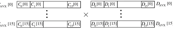
Assume that we want to compute 16 polynomial multiplications C0 ·D0, C1·D1, to C15·D15 where each polynomial has 16 coefficients. Also assume that the polynomials are stored in two AVX2-arraysCAV X andDAV X as shown
in Figure 3. The i-th coefficients of all Cj (and Dj) polynomials reside in the
same AVX2 vectors. With such an arrangement it is easy to compute the 16 polynomial multiplications in a batch by multiplying the elements ofCAV X and
DAV X. We design the polynomial multiplier routine with the aim to obtain such
an arrangement of coefficients during the threshold School-book multiplications. This is explained below.
The seven 64-coefficient polynomial multiplications in Algorithm 6 require 63 School-book multiplications of 16-coefficient polynomials. Since a 16-coefficient
0[0] D [0]
1
D D [0]
15
[15]
D 1 0[15]
D [15]
15 D C
AVX[0]
C AVX[15]
D AVX[0]
DAVX[15] [0]
1 15[0]
[15]
1
0[15] 15[15] 0[0]
C C C
C C
C
polynomial fits in an AVX2 vector, the 63 School-book multiplications can be computed in 4 batches using vectorized instructions. However, the batching is not trivial to implement. In the Karatsuba recursion, we do not immediately com-pute a School-book multiplication every time the recursion reaches the threshold condition. Instead, a lazy approach is adapted. We keep two ‘buckets’ each of which is an array of 16 AVX2 vectors. These buckets are gradually filled with the 16-coefficient polynomials that are the multiplicands of the School-book multi-plications. Once the buckets are full, each of them can be viewed as a 16×16 matrix, containing 256 coefficients. Next we transpose the matrices using a se-quence of AVX2 operations to reach the arrangement as shown in Figure 3. Now a batch multiplication is performed. The result is a collection of 31 vectors. This is again transposed to get the result of each 16-coefficient polynomial multipli-cation in two vectors. This lazy approach requires a bookkeeping which has a small overhead.
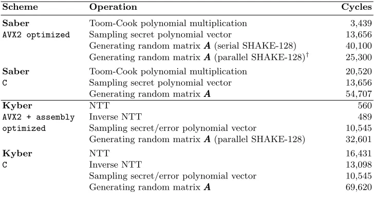
Table 2: Cycle count of the building blocks used in Saber and Kyber
Scheme Operation Cycles
Saber Toom-Cook polynomial multiplication 3,439
AVX2 optimized Sampling secret polynomial vector 13,656 Generating random matrixAAA(serial SHAKE-128) 40,100 Generating random matrixAAA(parallel SHAKE-128)† 25,300
Saber Toom-Cook polynomial multiplication 20,520
C Sampling secret polynomial vector 13,656
Generating random matrixAAA 54,707
Kyber NTT 560
AVX2 + assembly Inverse NTT 489
optimized Sampling secret/error polynomial vector 10,545 Generating random matrixAAA(parallel SHAKE-128) 32,601
Kyber NTT 16,431
C Inverse NTT 13,098
Sampling secret/error polynomial vector 10,545
Generating random matrixAAA 69,620
‡Not used in Saber, see Sec. 7
8
Results
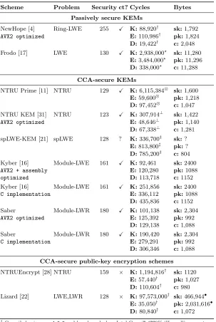
In Table 3, we compare our software implementation of Saber with software im-plementations of other lattice based post-quantum key exchange and encryption schemes. We compiled the Saber software usinggcc-7.1with optimization flags
multi-core support disabled on a Dell Latitude E7470 laptop with Ubuntu 16.04 operating system.
We remark that a totally fair comparison between the listed schemes and their software implementations is not possible since they are based on different hard problems, offer different levels of post-quantum security, implemented with different levels of optimizations and benchmarked on different platforms. Never-theless, it is clear from the table that Saber is highly efficient both in terms of bandwidth and computation time.
The implementations of Saber and Kyber use similar building blocks namely polynomial multiplication, generation of random matrix AAA, sampling of small secret (and error) polynomials and standard symmetric-key primitives for CCA transformations. In Table 2, we compare the performances of these building blocks excluding the symmetric-key primitives. Our Toom-Cook multiplication requires only 3,439 cycles. On the other hand, Kyber uses highly AVX-optimized NTT for polynomial multiplications. Furthermore, Kyber spends much less cy-cles in polynomial multiplications by generating the matrixAin the NTT domain directly and by keeping the secret polynomials in the NTT domain.
Saber does not require sampling of error polynomials, thus saving in com-putation time and entropy usage. As already described in Section 7 generating the random matrixAis faster in Saber (when same pseudorandom number gen-erator is used) since rejection sampling is not performed, resulting in optimal usage of random numbers. Though in this paper we consider only software im-plementation on high-end Intel processors, we would like to remark that random number generation is very expensive on resource-constrained platforms. When we compare the high-level C implementations of Saber and Kyber, we see that Saber performs better than Kyber.
Table 3:Performance and comparison of lattice-based KEMs and public-key encryption schemes. Cycles for key generation, encapsulation/encryption, and decapsulation/decryption are represented by K, E, and D respectively in the 5th column. Sizes of secret key (sk), public key (pk) and ciphertext (c) are reported in the last column. Constant-time implementations are marked withXin the columnct?. Performances are measured on the platform specified in the beginning of this section if not indicated otherwise.
Scheme Problem Security ct? Cycles Bytes
Passively secure KEMs
NewHope [4] Ring-LWE 255 X K:88,920† sk:1,792
AVX2 optimized E:110,986† pk:1,824
D:19,422† c:2,048
Frodo [17] LWE 130 X K:2,938,000? sk:11,280
E:3,484,000? pk:11,296 D:338,000? c:11,288
CCA-secure KEMs
NTRU Prime [11] NTRU 129 X K:6,115,384⊗ sk:1,600
E:59,600⊗ pk:1,218
D:97,452⊗ c:1,047
NTRU KEM [31] NTRU 123 X K:307,914⊥ sk:1,422
AVX2 optimized E:48,646⊥ pk:1,140
D:67,338⊥ c:1,281
spLWE-KEM [21] spLWE 128 ? K:336,700‡ sk:?
E:813,800‡ pk:?
D:785,200‡ c:804
Kyber [16] Module-LWE 161 X K:92,461 sk:2400
AVX2 + assembly E:120,280 pk:1088
optimized D:113,718 c:1152
Kyber [16] Module-LWE 161 X K:251,856 sk:2400
C implementation E:336,112 pk:1088
D:435,836 c:1152
Saber Module-LWR 180 X K:101,138 sk:2,304
AVX2 optimized E:125,392 pk:992
D:129,138 c:1,088
Saber Module-LWR 180 X K:190,420 sk:2,304
C implementation E:279,291 pk:992
D:306,346 c:1,088
CCA-secure public-key encryption schemes
NTRUEncrypt [28] NTRU 159 × K:1,194,816† sk:1120
E:57,440† pk:1,027
D:110,604† c:980
Lizard [22] LWE,LWR 128 × K:97,573,000† sk:466,944• E:35,050† pk:2,031,616•
D:80,840† c:1,072
†Compiled using
gcc-4.9.2and benchmarked on Intel Core i7-4770K (Haswell) computer
?Benchmarked on a 2.6GHz Intel Xeon E5 (Sandy Bridge) with hyperthreading enabled.
⊗Benchmarked on an Intel Haswell processor.
9
Acknowledgements
This work was supported in part by the Research Council KU Leuven: C16/15/058. In addition, this work was supported by the European Commission through the Horizon 2020 research and innovation programme under grant agreement No H2020-ICT-2014-645622 PQCRYPTO, H2020-ICT-2014-644209 HEAT, Cathe-dral ERC Advanced Grant 695305 and in part by Flemish Government, by the Hercules Foundation AKUL/11/19.
References
1. 2015., National Institute of Standards and Technology.: SHA-3 standard: Permutation-Based Hash and Extendable-Output Functions. FIPS PUB 202 (2015) 2. Albrecht, M.R.: On dual lattice attacks against small-secret lwe and parameter choices in helib and seal. In: EUROCRYPT 2017. pp. 103–129 (2017), https: //doi.org/10.1007/978-3-319-56614-6_4
3. Alkim, E., Ducas, L., P¨oppelmann, T., Schwabe, P.:NewHopewithout reconcili-ation (2016),http://cryptojedi.org/papers/#newhopesimple
4. Alkim, E., Ducas, L., P¨oppelmann, T., Schwabe, P.: Post-quantum key exchange – a new hope. In: USENIX Security 2016 (2016)
5. Alperin-Sheriff, J., Apon, D.: Dimension-preserving reductions from lwe to lwr. Cryptology ePrint Archive, Report 2016/589 (2016)
6. Alwen, J., Krenn, S., Pietrzak, K., Wichs, D.: Learning with rounding, revisited -new reduction, properties and applications. In: CRYPTO 2013. pp. 57–74 (2013), https://doi.org/10.1007/978-3-642-40041-4_4
7. Arora, S., Ge, R.: New algorithms for learning in presence of errors. In: Aceto, L., Henzinger, M., Sgall, J. (eds.) ICALP 2011. pp. 403–415 (2011),https://doi. org/10.1007/978-3-642-22006-7_34
8. Baan, H., Bhattacharaya, S., Garcia-Morchon, O., Rietman, R., Tolhuizen, L., Torre-Arce, J.L., Zhang, Z.: Round2: Kem and pke based on glwr. Cryptology ePrint Archive, Report 2017/1183 (2017),https://eprint.iacr.org/2017/1183 9. Bai, S., Galbraith, S.D.: Lattice Decoding Attacks on Binary LWE, pp. 322–337.
Springer International Publishing, Cham (2014), https://doi.org/10.1007/978-3-319-08344-5_21
10. Banerjee, A., Peikert, C., Rosen, A.: Pseudorandom functions and lattices. In: EUROCRYPT 2012. pp. 719–737 (2012), https://doi.org/10.1007/978-3-642-29011-4_42
11. Bernstein, D.J., Chuengsatiansup, C., Lange, T., van Vredendaal, C.: Ntru prime: reducing attack surface at low cost. Cryptology ePrint Archive, Report 2016/461 (2016),http://eprint.iacr.org/2016/461
12. Bhattacharya, S., Garcia-Morchon, O., Rietman, R., Tolhuizen, L.: spkex: An op-timized lattice-based key exchange. Cryptology ePrint Archive, Report 2017/709 (2017),http://eprint.iacr.org/2017/709
13. Birkett, J., Dent, A.W.: Relations among notions of plaintext awareness. In: PKC 2008. pp. 47–64 (2008),https://doi.org/10.1007/978-3-540-78440-1_4 14. Bodrato, M., Zanoni, A.: Integer and polynomial multiplication: Towards optimal
15. Bogdanov, A., Guo, S., Masny, D., Richelson, S., Rosen, A.: On the hardness of learning with rounding over small modulus. In: 13th International Conference on Theory of Cryptography. pp. 209–224 (2016), https://doi.org/10.1007/978-3-662-49096-9_9
16. Bos, J., Ducas, L., Kiltz, E., Lepoint, T., Lyubashevsky, V., Schanck, J.M., Schwabe, P., Stehl´e, D.: Crystals – kyber: a cca-secure module-lattice-based kem. Cryptology ePrint Archive, Report 2017/634 (2017), http://eprint.iacr.org/ 2017/634
17. Bos, J.W., Costello, C., Ducas, L., Mironov, I., Naehrig, M., Nikolaenko, V., Raghunathan, A., Stebila, D.: Frodo: Take off the ring! practical, quantum-secure key exchange from LWE. In: CCS 2016. pp. 1006–1018. ACM (2016), http://doi.acm.org/10.1145/2976749.2978425
18. Buchmann, J., Cabarcas, D., G¨opfert, F., H¨ulsing, A., Weiden, P.: Discrete ziggu-rat: A time-memory trade-off for sampling from a gaussian distribution over the integers. In: Revised Selected Papers on Selected Areas in Cryptography – SAC 2013 - Volume 8282. pp. 402–417. Springer-Verlag New York, Inc., New York, NY, USA (2014),http://dx.doi.org/10.1007/978-3-662-43414-7_20
19. Chen, L., Jordan, S.P., Liu, Y.K., Moody, D., Peralta, R.C., Perlner, R.A., Smith-Tone, D.C.: Report on post-quantum cryptography. In: NIST Internal Report (NI-STIR) - 8105 (2016),http://dx.doi.org/10.6028/NIST.IR.8105
20. Chen, Y., Nguyen, P.Q.: Bkz 2.0: Better lattice security estimates. In: ASIACRYPT 2011 (2011),https://doi.org/10.1007/978-3-642-25385-0_1
21. Cheon, J.H., Han, K., Kim, J., Lee, C., Son, Y.: A practical post-quantum public-key cryptosystem based on splwe. In: ICISC 2016. pp. 51–74 (2017),https://doi. org/10.1007/978-3-319-53177-9_3
22. Cheon, J.H., Kim, D., Lee, J., Song, Y.: Lizard: Cut off the tail! practical post-quantum public-key encryption from lwe and lwr. Cryptology ePrint Archive, Re-port 2016/1126 (2016),http://eprint.iacr.org/2016/1126
23. Diffie, W., Hellman, M.: New directions in cryptography. IEEE Transactions on Information Theory 22(6), 644–654 (Nov 1976)
24. Ding, J.: New cryptographic constructions using generalized learning with errors problem. Cryptology ePrint Archive, Report 2012/387 (2012), http://eprint. iacr.org/2012/387
25. Ducas, L., Durmus, A., Lepoint, T., Lyubashevsky, V.: Lattice signatures and bimodal gaussians. In: Canetti, R., Garay, J.A. (eds.) Advances in Cryptology – CRYPTO 2013: 33rd Annual Cryptology Conference, Santa Barbara, CA, USA, August 18-22, 2013. Proceedings, Part I, pp. 40–56. Springer Berlin Heidelberg, Berlin, Heidelberg (2013),http://dx.doi.org/10.1007/978-3-642-40041-4_3 26. Ducas, L., Nguyen, P.Q.: Faster gaussian lattice sampling using lazy floating-point
arithmetic. In: Wang, X., Sako, K. (eds.) Advances in Cryptology – ASIACRYPT 2012: 18th International Conference on the Theory and Application of Cryptology and Information Security, Beijing, China, December 2-6, 2012. Proceedings, pp. 415–432. Springer Berlin Heidelberg, Berlin, Heidelberg (2012), http://dx.doi. org/10.1007/978-3-642-34961-4_26
27. Dwarakanath, N.C., Galbraith, S.D.: Sampling from discrete gaussians for lattice-based cryptography on a constrained device. Applicable Algebra in Engineering, Communication and Computing 25(3), 159–180 (2014), http://dx.doi.org/10. 1007/s00200-014-0218-3
29. Hoffstein, J., Pipher, J., Silverman, J.H.: Ntru: A ring-based public key cryptosys-tem. In: AANTS-III (1998),https://doi.org/10.1007/BFb0054868
30. Hofheinz, D., H¨ovelmanns, K., Kiltz, E.: A modular analysis of the fujisaki-okamoto transformation. Cryptology ePrint Archive, Report 2017/604 (2017), http://eprint.iacr.org/2017/604
31. H ulsing, A., Rijneveld, J., Schanck, J.M., Schwabe, P.: High-speed key encap-sulation from ntru. Cryptology ePrint Archive, Report 2017/667 (2017), http: //eprint.iacr.org/2017/667
32. Jiang, H., Zhang, Z., Chen, L., Wang, H., Ma, Z.: Post-quantum ind-cca-secure kem without additional hash. Cryptology ePrint Archive, Report 2017/1096 (2017), https://eprint.iacr.org/2017/1096
33. Jin, Z., Zhao, Y.: Optimal key consensus in presence of noise. Cryptology ePrint Archive, Report 2017/1058 (2017),https://eprint.iacr.org/2017/1058 34. Karmakar, A., Roy, S.S., Reparaz, O., Vercauteren, F., Verbauwhede, I.:
Constant-time discrete gaussian sampling. IEEE Transactions on Computers pp. 1–1 (2018) 35. Kirchner, P., Fouque, P.: An improved BKW algorithm for LWE with applications to cryptography and lattices. In: CRYPTO 2015. pp. 43–62 (2015),https://doi. org/10.1007/978-3-662-47989-6_3
36. Langlois, A., Stehl´e, D.: Worst-case to average-case reductions for module lattices. Designs, Codes and Cryptography 75(3), 565–599 (Jun 2015),https://doi.org/ 10.1007/s10623-014-9938-4
37. Lyubashevsky, V., Peikert, C., Regev, O.: On ideal lattices and learning with er-rors over rings. In: EUROCRYPT 2010 (2010), https://doi.org/10.1007/978-3-642-13190-5_1
38. Micciancio, D., Walter, M.: Gaussian sampling over the integers: Efficient, generic, constant-time. Cryptology ePrint Archive, Report 2017/259 (2017), http:// eprint.iacr.org/2017/259
39. Peikert, C.: An efficient and parallel gaussian sampler for lattices. In: Rabin, T. (ed.) Advances in Cryptology – CRYPTO 2010: 30th Annual Cryptology Con-ference, Santa Barbara, CA, USA, August 15-19, 2010. Proceedings, pp. 80–97. Springer Berlin Heidelberg, Berlin, Heidelberg (2010), http://dx.doi.org/10. 1007/978-3-642-14623-7_5
40. Peikert, C.: Lattice cryptography for the internet. In: Mosca, M. (ed.) PQCrypto 2014 (2014),https://doi.org/10.1007/978-3-319-11659-4_12
41. Regev, O.: On lattices, learning with errors, random linear codes, and cryptog-raphy. In: STOC ’05. pp. 84–93. ACM (2005), http://doi.acm.org/10.1145/ 1060590.1060603
42. Saito, T., Xagawa, K., Yamakawa, T.: Tightly-secure key-encapsulation mecha-nism in the quantum random oracle model. Cryptology ePrint Archive, Report 2017/1005 (2017),https://eprint.iacr.org/2017/1005
43. Schnorr, C.P., Euchner, M.: Lattice basis reduction: Improved practical algorithms and solving subset sum problems. Mathematical Programming (1994),https:// doi.org/10.1007/BF01581144
45. Stehl´e, D., Steinfeld, R.: Making ntru as secure as worst-case problems over ideal lattices. In: EUROCRYPT 2011 (2011), https://doi.org/10.1007/978-3-642-20465-4_4
46. Targhi, E.E., Unruh, D.: Post-quantum security of the fujisaki-okamoto and oaep transforms. In: Theory of Cryptography: 14th International Conference (2016), https://doi.org/10.1007/978-3-662-53644-5_8
A
Toom-Cook-4 polynomial multiplication.
Here we describe the Toom-Cook polynomial multiplication used in our imple-mentation.
Algorithm 6: Toom-Cook Algorithm
Input:Two polynomialsA(x) andB(x)of degreen= 256
Output:C(x) =A(x)∗b(x)
// Splitting A(x) into four polynomials of size 64
1 A(y) =A3·y3+A2·y2+A1·y+A0 wherey=x64 // Splitting B(x) into four polynomials of size 64
2 B(y) =B3·y3+B2·y2+B1·y+B0
// Evaluation of the polynomials at y={0,±1,±1
2,2,∞}. These multiplications are computed using Karatsuba
3 w1 =A(∞)∗B(∞) =A3∗B3
4 w2 =A(2)∗B(2) = (A0+ 2·A1+ 4·A2+ 8·A3)∗(B0+ 2·B1+ 4·B2+ 8·B3)
5 w3 =A(1)∗B(1) = (A0+A1+A2+A3)∗(B0+B1+B2+B3)
6 w4 =A(−1)∗B(−1) = (A0−A1+A2−A3)∗(B0−B1+B2−B3)
7 w5 =A(12)∗B(12) = (8·A0+ 4·A1+ 2·A2+A3)∗(8·B0+ 4·B1+ 2·B2+B3)
8 w6 =A(−21)∗B(−21) = (8·A0−4·A1+ 2·A2−A3)∗(8·B0−4·B1+ 2·B2−B3)
9 w7 =A(0)∗B(0) =A0∗B0 // Interpolation
10 w2 =w2+w5
11 w6 =w6−w5
12 w4 = (w4−w3)/2
13 w5 =w5−w1−64·w7
14 w3 =w3+w4
15 w5 = 2·w5+w6
16 w2 =w2−65·w3
17 w3 =w3−w7−w1
18 w2 =w2+ 45·w3
19 w5 = (w5−8·w3)/24
20 w6 =w6+w2
21 w2 = (w2+ 16·w4)/18
22 w3 =w3−w5
23 w4 =−(w4+w2)
24 w6 = (30·w2−w6)/60
25 w2 =w2−w6