Analytic solutions for free vibration analysis of laminated beams in three-dimensional statement

Analytic solutions for free vibration analysis of laminated

beams in three-dimensional statement

SergeyGolushko1,2,∗_,GlebGorynin3_{, andArseniyGorynin}1

1_{Novosibirsk State University}

2_{Institute of Computational Technologies of SB RAS} 3_{Surgut State University}

Abstract.In this research we consider free vibrations of laminated beams in terms of three-dimensional linear theory of elasticity. Analytic solutions for natural frequencies of laminated beams are obtained by using an asymptotic splitting method. The results were compared with classical Euler“Bernoulli beam theory and Timoshenko beam theory.

1 Introduction

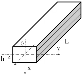
Let us consider a free vibrations of laminated beam (Fig. 1) with an arbitrary cross section constant along the length and symmetric aboutOxaxis. The beam consists of arbitrary num-ber of isotropic layers. The layers are counted from top to bottom alongOxaxis. The origin of coordinates is located in center of mass of cross section. Let denote number of layers bys, the layer number byi, the displacements along the x-, y-, and z-axes byux,uy,uz, respectively and the length and height of the beam byLandh.

We will use dimensionless variables and functions, keeping the original notation for sim-plicity:

ε=h/L, x↔ x

h, y↔

y

h, z↔ z h, uα↔

uα

˜

u, λi↔

λi ˜ E,

µi↔

µi ˜

E, σαβ↔

σαβ

σ0

, σ0=

˜ Eu˜

h , ρi↔

ρiuh˜ ˜ Et2

0

, t↔ t

t0

, ωn↔ωnt0,

(1)

where ˜E – is a characteristic value of YoungTM_{s modulus, ˜u – is a characteristic value for}

displacementux,σαβ – are the components of the linear stress tensor, ωn – is the natural frequency of the beam,t0 - is characteristic time,ρi,µi,λi– are the density and the elastic constants of the material of thei-th layer. ε– is a small parameter. Herein after we assume that :α∈(x, y,z), i= 1, . . . , s.

The dimensionless equations of motion of a beam with no mass loads are:

−ρi

∂2_(u α)i

∂t2 +

∂(σαx)i

∂x +

∂(σαy)i

∂y +ε ∂(σαz)i

∂z =0. (2)

Figure 1.Laminated beam

Boundary conditions on the lateral surfaces of the beam (except for the ends):

(σαx)inx+(σαy)iny=0. (3)

The interfacial stresses (σαn)iand displacements (uα)iare continuous:

[(σαn)] j

i =0, (σαn)i=(σαx)inx+(σαy)iny, (uα)j=(uα)i. (4)

The material of each layer obeys HookeTM_{s law:}

(σαβ)i=λiθδαβ+2µieαβ, θ=

3 X

γ=1

eγγ, λi=

νiEi

(1−2νi)(1+νi), µi= Ei

2(1+νi), (5)

whereeαβare the components of the linear strain tensor.

Cauchy equations for the linear strain tensor:

(exx)i= ∂(ux)i

∂x , (eyy)i=

∂(uy)i

∂y , (ezz)i=ε ∂(uz)i

∂z , (exy)i= 1 2(

∂(ux)i

∂y + ∂(uy)i

∂x ),

(exz)i=1 2(ε

∂(ux)i

∂z +

∂(uz)i

∂x ), (eyz)i= 1 2(ε

∂(uy)i

∂z +

∂(uz)i

∂y ).

(6)

Together formulas (2) – (6) represent a linear elasticity boundary-value problem in Saint-Venant’s statement.

(uβ)(in)(¯r,t, ε)= n+1 X

k=0

(Uβ)(2i k)

∂2k_u(n) 0

∂z2k ε

2k_,(uz)(n)

i (¯r,t, ε)= n

X

k=0

(Uz)(2_ik+1)∂

2k+1_u(n) 0

∂z2k+1 ε 2k+1_,

β∈(x, y), (Ux)

(0)

i =1, (Uy)

(0)

i =0, (Uz)

(1)

i =−(x−c0),

(σαβ)(_in)(¯r,t, ε)= n+1 X

k=1

(ταβ)(2_i k)∂

2k_u(n) 0

∂z2k ε

2k_,

(σzz)(_in)(¯r,t, ε)= n

X

k=1

(τzz)(2_i k)∂

2k_u(n) 0

∂z2k ε

2k_,

(σαz)

(n)

i (¯r,t, ε)= n

X

k=1

(ταz)

(2k+1)

i

∂2k+1_u(n) 0

∂z2k+1 ε

2k+1_{, α, β∈(x, y),}

(7)

where (Uα)(_ik) are the characteristic functions of the displacement vector; (uα)_i(n)(¯r,t, ε) are the displacement components of thei–th layer in then–th order asymptotic approximation; (ταβ)(_ik)(x, y) are the characteristic functions of the tensor stress field in the beam cross section; u0(z,t) is the deflection function.

Relations between characteristic functions (ταβ)(_ik)(x, y) and characteristic functions (Uα)(ik):

(τxy)2ik=µi(

∂(Uy)(2_i k)

∂x +

∂(Ux)(2_i k)

∂y ), (τzα)2ik+1=µi(

∂(Uz)(2_i k+1)

∂α +(Uα)

(2k)

i ),

(τzz)2_ik=(λi+2µi)(Uz)(2_i k−1)+λi(

∂(Ux)

(2k)

i

∂x +

∂(Uy)(2i k)

∂y ), (8)

(τxx)2ik=(λi+2µi)

∂(Ux)(2_i k)

∂x +λi((Uz)

(2k−1)

i +

∂(Uy)(2_i k)

∂y ),

(τyy)2_ik=(λi+2µi)

∂(Uy)(2_ik)

∂y +λi((Uz)

(2k−1)

i +

∂(Ux)(2_i k)

∂x ).

In case of free vibrations transverse the distributed load is equal to zero. According to the approximation (7), equation of free vibrations looks as follows [3]:

M∂

2_u(n) 0

∂t2 +

n+1 X

k=2

G(2_xzk−1)∂

2k_u(n) 0

∂z2k ε

2k_{=0, G}(2k−1)

xz =−

s

X

i=1 Z

Fi

(τxz)(2_i k−1)dF, (9)

whereG(2xzk−1) are the characteristic stiffnesses of the cross section; M is the dimensionless mass of the beam cross section per unit length. To find equation of free vibrations (9) it is necessary to determine characteristic stiffnesses by solving several boundary-value problems in the beam cross section.

2 Boundary-value problems in the beam cross section

Approximation of displacement vector and stress tensor of the form (7) allow us to split the original three-dimensional problem into the (n+1) much easier two-dimensional problems, where the unknowns are characteristic functions (ταβ)(_in). The characteristic numberkchanges from 1 ton+1. The first two boundary-value problems are described below.

with numberk=1:                 

∂(ταx)

(2)

i

∂x +

∂(ταy)(2)i

∂y =0, ∂(τzx)(3)_i

∂x +

∂(τzy)(3)_i

∂y +(τzz)

(2)

i =0;

(10)

with numberk=2:

                          

∂(τxx)(4)_i

∂x +

∂(τxy)(4)_i

∂y +(τxz)

(3)

i +ρi

G(3)xz M =0,

∂(τxy)(4)_i

∂x +

∂(τyy)(4)_i

∂y +(τyz)

(3)

i =0.

∂(τzx)

(5)

i

∂x +

∂(τzy)

(5)

i

∂y +(τzz)

(4)

i −ρi

G(3)xz

M (x−c0)=0;

(11)

Boundary conditions on the border of cross section for (10), (11):

(ταx)

(2k)

i nx+(ταy)

(2k)

i ny=0, (τzx)

(2k+1)

i nx+(τzy)

(2k+1)

i ny=0, α∈(x, y). (12)

Conditions at the interface between layers for (10), (11):

(τnβ)(2_ik) =(τnβ)(2_jk), (τnz)_i(2k)=(τnz)(2_jk),

(Uβ)(2_i k)=(Uβ)(2_jk), (Uz)_i(2k+1)=(Uz)(2_jk+1), α∈(x, y,z), β∈(x, y). (13)

According to [2] approximation of displacement vector and stress tensor of the form (7) with consideration to (10)-(13) gives an asymptotic solution of linear elasticity problem (2)-(6) with residual proportional toε(2n+2)_.

The following equalities are fulfilled [4]:

(τzz)(2)_i =ν(τxx)(2)_i +ν(τyy)(2)_i −Ei(x−c0),

(τzz)

(4)

i =ν(τxx)

(4)

i +ν(τyy)

(4)

i +Ei(Uz)

(3)

i .

(14)

Equations (10), (11) with (12), (13) represent boundary-value problems in the beam cross section fork=1, 2. In case of arbitrary cross section it is necessary to use numerical methods for solving corresponding boundary-value problems. However for widely used types of cross sections as a rectangular or I-beam cross sections it is possible to find an analytic solution.

3 Solution for rectangular cross section

From the equation of vibrations (9) follows the formula of natural frequencies for a hinged simple beam of an arbitrary cross section [3]:

ω(n)

m =

v u tn+1

X

k=2

G(2xzk−1)(πmε)2k(−1)k,

ω(1)

m =(πmε)

2 s

G(3)xz

M , ω

(2)

m =ω

(1)

m

s

1−G (5)

xz

G(3)xz (πmε)2,

(15)

a) b)

Figure 2.) – I-beam cross section; b) – rectangular cross section

To findω(1)m, ω

(2)

m it is necessary to solve first two boundary-value problems in the beam cross section fork=1, 2 and determine characteristic stiffnessesG(3)xz,G

(5)

xz. First boundary-value problem (10), (12), (13) fork=1 has an exact solution:

(τzz)(2)_i =−(x−c0)Ei, (ταα)(2)_i =0, α∈(x, y),

(Ux)(2)_i =0.5(−νy2+ν(x−c0)2+C2), Z

F

(Ux)(2)_i dF=0, (Uy)(2)_i =νy(x−c0).

(16)

Constantc0need to be determined from condition:

Z

Fi

h(τzz)(2)_i idF=0. (17)

ForG(3)xz with consideration to (16) the following formula is satisfied:

G(3)_xz =−

s

X

i=1 Z

Fi

(τxz)(3)_i dF=−

s

X

i=1 Z

Fi

x(τzz)(2)_i dF=[EI], [EI]= s

X

i=1

EiIi. (18)

Formulas (16), (18) are satisfied for an arbitrary cross section. It means that solution of a first boundary-value problem does not depend on a form of cross section.

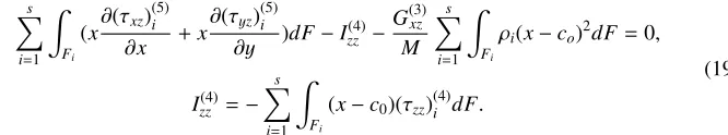
To findG(5)xz we multiply the third equality (11) by (x−c0) and integrate over the entire

beam cross section:

s

X

i=1 Z

Fi

(x∂(τxz)

(5)

i

∂x +x

∂(τyz)(5)_i

∂y )dF−I

(4)

zz −

G(3)xz M

s

X

i=1 Z

Fi

ρi(x−co)2dF=0,

Izz(4)=− s

X

i=1 Z

Fi

(x−c0)(τzz)

(4)

i dF.

(19)

Introducing xunder the derivative sign and replacing the integral over cross section to the integral over the boundary of cross section, we obtain the formula:

G(5)_xz =I_zz(4)+G

(3)

xz

M [ρI], [ρI]= s

X

i=1

ρiIi= s

X

i=1 Z

Fi

To determineIzz in formula (20) it is necessary to take into account the cross-sectional shape. To solve the subsequent boundary-value problems, we use the procedure of averaging the characteristic functions over the cross section. The sought stresses will vary slightly within the thin wall and it can be assumed that their average values will almost coincide with the values themselves. A similar procedure for solving boundary value problems is described in [5].

Here we present a solution for a thin-walled rectangular beams. The procedure of aver-aging the characteristic functions over the cross section looks as follows:

hfi=1

b

Z 0.5b

−0.5b

f(α,s)ds. (21)

Apply the averaging procedure (21) to the second equation (11) to find unknown char-acteristic functions (τzx)

(3)

i (τzy)

(3)

i . We use the conditions on the lateral surface of the beam (11) and take into account the solution (16):

dh(τzx)

(3)

i i

dx =xEi, h(τzx)

(3)

i i=

Z x

−0.5

Eiξdξ. (22)

The function (τzy)

(3)

i is antisymmetric across the width of the cross section, therefore (τzy)(3)i =0. We average the second equality (8) and substitute in it the averaged third expres-sion from (16), integrate over the variablexand express the averaged characteristic function (Uz)(3)_i :

h(Uz)i(3)_i =

Z x

−0.5 (h(τzx)

(3)

i i

µi

− h(Ux)(2)_i i)dξ+C1, h(Ux)(2)_i i=0.5ν(x2−

1

12). (23)

The constantC1in the expression (23) can be found from the equality:

Z 0.5

−0.5 h(τzz)

(4)

i idx=0. (24)

The expression (24) follows from the fact that with pure bending, the longitudinal force is zero.

We now proceed to the second boundary value problem. We average the first equation (11) and use the conditions at the cross section boundary (12):

d(hτ_xx)(4)_i i

dx +h(τzx)

(3)

i i+

G(3)xz

M hρii=0, h(τxx)

(4)

i i|x=−0.5=0. (25)

We integrate (25) and get:

h(τxx)(4)_i i=−

Z x

−0.5

(h(τzx)(3)_i idξ−G (3)

xz M

Z x

−0.5

hρ_iidξ. (26)

Due to antisymmetry, the average values of the following functions are zero:

h(τyy)(4)_i i=0, h(τxy)(4)_i i=0. (27)

We average the second expression over the width of the cross section (14):

h(τzz)(4)_i i=νh(τxx)(4)_i i+Eih(Uz)(3)_i i. (28)

4 Analysis of the solution

To compare the obtained results, we consider two theories of free vibrations of a homoge-neous beam: the classical Euler“Bernoulli beam theory and Timoshenko beam theory. The difference between TimoshenkoTMs theory is that it takes into account the deplanation and in-ertia of the rotation of the cross section during vibrations [1]. The equation of free vibrations of a homogeneous beam in TimoshenkoTMs theory is as follows [6]:

EI

ρF

∂4_u 0

∂z4 +

∂2_u 0

∂t2 −

I F(1+

E k0_G)

∂4_u 0

∂z2_t2 +

ρI k0_GF

∂4_u 0

∂t4 =0, k

0₌ 10(1+ν)

12+11ν, (29)

whereGis a shear modulus;k0_{is a coefficient depending on the shape of the cross section.} The formula for calculating the natural frequencies of a hinged simple beam::

ωT

m=a

π2_m2

L2 [1−

1 2

Iπ2_m2

FL2 (1+

E

k0_G)], a=

s

EI

ρF. (30)

The first and the second approximations of natural frequency (15) in dimensional vari-ables are:

ω(1)

m =[a]

π2_m2

L2 , ω (2)

m =[a]

π2_m2

L2 r

1−ζπ 2_m2_h2

L2 , [a]= s

[EI] [ρF], ζ=

G(5)xz

[EI]. (31)

In case of homogeneous beam the frequency ω(1)m is equal to the frequency predicted by classical beam theory based on the Bernoulli hypothesis. The frequencyω(2)m takes into account the deplanation and inertia of the rotation of the cross section.

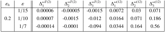
Let us compare two formulas (31) and (30) in case of homogeneous beam. To do that, we introduce relative differences∆ω_mbetween natural frequencies:

∆ω(2)T

m =

(ω(2)m −ω

(T)

m )

ω(2)

m

, ∆ω(12)

m =

(ω(1)m −ω

(2)

m)

ω(2)

m

, εh= b

h, (32)

whereεh 1 is a ratio between width and height of the cross section. It is important to note that the formulas (31) are applicable as long as the condition is true:

(πmε)<1. (33)

The expression (33) imposes a restriction on the length of the beam and the ordinal number of the frequency.

Table 1.Relative differences for homogeneous beam,ν=0.25

εh ε ∆

ωT(2)

1 ∆

ωT(2)

2 ∆

ωT(2)

3 ∆

ω(12)

1 ∆

ω(12)

2 ∆

ω(12) 3 1/15 0.00006 -0.00005 -0.0015 0.0072 0.03 0.071

0.2 1/10 0.00007 -0.0015 -0.012 0.0164 0.071 0.186

1/7 -0.00014 -0.0001 -0.094 0.0344 0.164 0.56

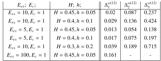
Eex; Ec; H;h; ∆₁ω(12) ∆ω₂(12) ∆ω₃(12)

Eex=10,Ec=1 H=0.45,h=0.05 0.02 0.087 0.237

Eex=10,Ec=1 H=0.4,h=0.1 0.029 0.136 0.424

Eex=5,Ec=1 H=0.45,h=0.05 0.013 0.054 0.138

Eex=5,Ec=1 H=0.4,h=0.1 0.017 0.075 0.197

Eex=10,Ec=1 H=0.3,h=0.2 0.039 0.189 0.715

Eex=100,Ec=1 H=0.45,h=0.05 0.161 -

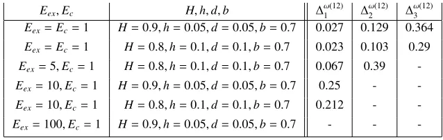
-In Table 2 the results for a three-layer beam consisting of isotropic materials are presented. It is assumed that the Young’s modulus of the outer layers is larger than in the middle layer (Eex > Ec) and Poisson’s coefficients of the layers are equal. The thickness of the layers varies. It can be seen that the more different the mechanical characteristics of the layers, the higher the relative differences. For a three-layer beam, in which the Young’s modules differ 100 times, the relative error for the first natural frequency reaches 16%. Thus, the use of second-order asymptotic approximations and higher is more justified for non-homogeneous beams.

A situation may arise when the magnitude under the root in the formula (15) becomes negative. In this case, the lower bound for the true frequency will be zero. In such cases, there is a dash in the table.

4.1 Solution for I-beam cross section

Similar to a beam of rectangular section, an I-beam was calculated. The averaging of char-acteristic functions was carried out over the wall widthdand over the height of the shelves h.

In Table 3 the relative differences of natural frequencies for a homogeneous I-beam are presented. It can be seen that the natural frequencies predicted by the second asymptotic approximation are almost equal to the ones predicted by Timoshenko theory. The difference between them is small and does not exceed 3%.

Here we present the results for a three-layer non-homogeneous I-beam (Table 4), in which the wall is made of one material and the shelves are of another. The effect of cross section deplanation in this case increases. When the Young’s modulus differs 10 times, the relative differences for the first frequency reaches 25%.

5 Conclusions

The asymptotic splitting method allows to obtain the first approximations of the natural fre-quenciesω(mn) analytically when the Poisson’s coefficients in each layer are equal. The first approximationω(1)m corresponds to the frequencies predicted by the classical theory of the Bernoulli-Euler beam and estimate the true frequency from above. The second approxima-tionω(2)m takes into account the deplanation and inertia of the rotation of the cross section during vibrations and evaluates the true frequency from below. For a hinged simple homo-geneous beam, the second approximationω(2)m almost completely coincides with the solution obtained from the refined Timoshenko theory.

Table 3.Relative differences for homogeneous I-beam,ν=0.25,En=Ec

ε H,h,d,b ∆₁ω(2T) ∆ω₂(2T) ∆ω₃(2T) H=0.8,h=0.1,d=0.1,b=0.7 0.002 0.006 0.003

ε=1/15 H=0.9,h=0.05,d=0.05,b=0.7 0.001 0.001 -0.03 H=0.8,h=0.1,d=0.1,b=0.5 -0.003 -0.004 -0.02

H=0.8,h=0.1,d=0.1,b=0.5 0.005 0.018 0.034

H=0.8,h=0.1,d=0.1,b=0.7 0.006 -0.28

-ε=1/7 H=0.9,h=0.05,d=0.05,b=0.7 -0.0002 -1.1 -H=0.8,h=0.1,d=0.1,b=0.5 -0.005 -0.22

-H=0.8,h=0.1,d=0.1,b=0.5 0.02 0.016

-Table 4.Relative differences for non-homogeneous I-beam,ν=0.25, ε=1/15

Eex,Ec H,h,d,b ∆

ω(12)

1 ∆

ω(12)

2 ∆

ω(12) 3 Eex=Ec=1 H=0.9,h=0.05,d=0.05,b=0.7 0.027 0.129 0.364

Eex=Ec=1 H=0.8,h=0.1,d=0.1,b=0.7 0.023 0.103 0.29

Eex=5,Ec=1 H=0.8,h=0.1,d=0.1,b=0.7 0.067 0.39

-Eex=10,Ec=1 H=0.9,h=0.05,d=0.05,b=0.7 0.25 -

-Eex=10,Ec=1 H=0.8,h=0.1,d=0.1,b=0.7 0.212 -

-Eex=100,Ec=1 H=0.9,h=0.05,d=0.05,b=0.7 - -

-section is not large and the classical theory can be used with an acceptable accuracy. The insignificant difference in the results can be explained by the fact that for isotropic materials the effect of transverse deformations is small.

The research was supported financially by Russian Foundation for Basic Research, Project 18-29-18029

References

[1] S. P. Timoshenko, W. Weaver Jr. , D. H. YoungVibration Problems in Engineering// John Wiley Sons, 1990 – pp. 624.

[2] Gorynin G.L., Nemirovsky Yu.V.Spatial tasks of bending and torsion of layered struc-tures. Asymptotic splitting method. – Novosibirsk, 2004. – 409 p. (in Russian)

[3] Gorynin G.L., Nemirovsky Yu.V. Tranverse vibration of laminated beams in Three-Dimensional Formulation//Int. Appl. Mech. – 2005. – 41, N. 6. – P. 631-645.

[4] Gorynin G.L., Nemirovsky Yu.V. Deformation of laminated anisotropic bars in the three-dimensional statement 1.Transverse-longitudinal bending and edge compatibility condition//Mechanics of Composite Materials, Vol. 45, N. 3, 2009. – pp. 257-280. [5] Gorynin G.L., Gorynina O.G.The study of the stress-strain state of a three-layer

I-beam in three-dimensional statement//Vestnik Sibadi. – 2012. – N. 5 (27). – pp. 49-54. (in Russian)