R E S E A R C H
Open Access
Modeling individual HRTF tensor using high-order
partial least squares
Qinghua Huang
*and Lin Li
Abstract
A tensor is used to describe head-related transfer functions (HRTFs) depending on frequencies, sound directions, and anthropometric parameters. It keeps the multi-dimensional structure of measured HRTFs. To construct a multi-linear HRTF personalization model, an individual core tensor is extracted from the original HRTFs using high-order singular value decomposition (HOSVD). The individual core tensor in lower-dimensional space acts as the output of the multi-linear model. Some key anthropometric parameters as the inputs of the model are selected by Laplacian scores and correlation analyses between all the measured parameters and the individual core tensor. Then, the multi-linear regression model is constructed by high-order partial least squares (HOPLS), aiming to seek a joint subspace approximation for both the selected parameters and the individual core tensor. The numbers of latent variables and loadings are used to control the complexity of the model and prevent overfitting feasibly. Compared with the partial least squares regression (PLSR) method, objective simulations demonstrate the better performance for predicting individual HRTFs especially for the sound directions ipsilateral to the concerned ear. The subjective listening tests show that the predicted individual HRTFs are approximate to the measured HRTFs for the sound localization.
Keywords:Head-related transfer function; Tensor; Multi-linear model; Laplacian score; High-order partial least squares
1 Introduction
The generation of virtual three-dimensional (3D) audio based on head-related transfer functions (HRTFs) be-comes important in many applications, such as PC entertainment, hearing aids, multimedia, and virtual real-ity, with spatial and immersive feelings in 3D auditory space. Its key technique is to recover the location informa-tion of a sound source by HRTFs. HRTFs describe the spectral changes of sound waves from the sound positions to a listener's ear carnal, due to the diffraction and reflec-tion properties of the anthropometric structures. The corresponding representations in the time domain are head-related impulse responses (HRIRs). HRTFs not only vary with sound source locations (elevations and azimuths) and frequencies but also depend on external physiological structures uniquely from one listener to another. The tiny difference of anthropometric structures can create a significant influence on HRTFs for sound localization.
Perceptual distortions may occur in spatial sound localization with non-individual HRTFs. Unfortunately, individual HRIR measurements for each listener are very time consuming and difficult to implement with specific instruments. So, it is not practical and economical for various applications. It is essential to obtain individual HRTFs fast and effectively.
Some theoretical calculation methods were used to generate individual HRTFs based on a snowman model [1] and the boundary element method (BEM) [2], which are unsuitable for the individual HRTF estimation at high frequencies. They also need a large amount of calculations and have a high request for computers [3]. To customize HRTFs more easily and effectively, some researchers attempted to explore the effect resulting from the differ-ence of anthropometric structures on HRTFs [4-6] and further study the relationship between HRTFs and an-thropometric parameters [7,8]. Zotkin et al. measured the pinna size of a new subject and used the similarity of pinna structures between the new subject and the listeners in a known HRTF database to select the best matching HRTFs as the individual HRTFs of that subject [9]. Zeng * Correspondence:[email protected]
School of Communication and Information Engineering, Shanghai University, Shanghai 200072, People's Republic of China
et al. applied a hybrid algorithm for selecting the individ-ual HRTFs based on the similarity of anthropometric structures [10]. These HRTF personalization methods based on database matching were limited by the sizes of the existing databases and the matching criteria. Conse-quently, individual modeling based on anthropometric measurements is a big breakthrough in HRTF customiza-tion. HRTF estimation has three indispensable parts in-cluding the dimension reduction of original HRTFs, a reasonable selection of anthropometric measurements, and the mapping relation between the compacted HRTFs and the selected anthropometric measurements.
HRTFs depend on frequencies, sound directions (azi-muths and elevations), and listeners. The collection of high-spatial-resolution HRTFs of each listener makes up a large dataset with a multi-dimensional structure and complex characteristic. It is difficult to directly apply the original HRTFs into learning and storing. Due to the high dimensionality, it is necessary to extract the indi-vidual factors with lower dimension from the original HRTFs and get rid of non-individual features. Principal component analysis (PCA) was popularly applied to get individual weight coefficients and basis vectors before the HRTF customization [11-15]. Sodnik et al. found a suitable representation for the weight variations of the HRTF amplitudes by PCA [16]. Wang et al. applied PCA for the HRTF compression [17] and interpolation [18], respectively. Xie presented to recover the high-spatial-resolution HRTFs from the individual weight coefficients by a small set of measurements [19]. Kistler and Wightman modeled the HRTF matrix by PCA [20]. PCA successfully reduces the dimensionality of HRTF datasets and it is based on the so-called vector space model. Under this model, the HRTFs of a subject at different source loca-tions are modeled as a vector and the collection of indi-vidual HRTFs is modeled as a matrix. It cannot capture the variations among different sound source directions and the interaction of multiple variables in HRTFs. To overcome the weakness of the vector model, Grindlay and Vasilescu modeled HRTFs using a multi-factor (tensor) representation [21]. The tensor framework is used to learn the interaction of the multi-variable for HRTF representa-tion and can achieve the dimensionality reducrepresenta-tion of the HRTF dataset along each variable separately. Rothbucher et al. used multi-way array analysis to customize HRTFs [22]. There is no specific selection of anthropometric pa-rameters in combination with the HRTF tensor. However, the key parameter selection is important for the accuracy of HRTF model estimation.
A number of anthropometric parameters (head, torso, pinna, etc.) affect the immersion of listener's spatial hearing and show different influence on HRTFs. It is un-desirable to apply all the anthropometric measurements for modeling the individual HRTFs. A reasonable selection
of the anthropometric measurements is necessary to the individual HRTF customization. Xu et al. [5] found that ear parameters were significantly correlated with the mag-nitudes of HRTFs at high frequencies. Chen et al. studied the influence of the neck and torso parameters on the near-field HRTFs [23]. Rothbucher et al. [7] developed a measurement system that was capable to scan a human body for the anthropometric measurements. Hu et al. used correlation coefficients twice for the parameter selec-tion and retained eight parameters for the HRTF estima-tion [12,24,25]. Zeng et al. [10] also selected 13 reference physiological parameters utilizing correlation analyses be-tween the measured HRTFs and all the anthropometric parameters for matching the best HRTFs. Xu et al. [26] used a weighted correlation method and selected eight sig-nificant parameters. Hugeng and Gunawan [27] analyzed the correlation among anthropometric parameters and three physical quantities (interaural time difference, interaural level difference, and pinna notch frequency). However, correlation analyses only describe the linear re-lationship among anthropometric parameters and cannot evaluate the significance of a single parameter. These existing methods for the parameter selection did not con-sider the relation between the anthropometric parameters and the multi-dimensional HRTFs. In order to avoid the HRTF vector modeling, it is necessary to keep the multi-dimensional structure of the original HRTFs and on this basis to select the key parameters.
back-propagation artificial neural network (ANN) was used to HRTF personalization. Huang et al. applied support vec-tor regression (SVR) to model personalized HRIRs [30,31]. All these linear or non-linear HRTF personaliza-tion methods were based on the vector model to cus-tomize HRTFs. They are unable to establish the mapping from anthropometric parameters to a HRTF tensor. In order to predict the individual HRTFs of dif-ferent sound directions, it requires a separate regression model for each sound direction. A high-spatial-resolution HRTF prediction based on the tensor model requires only one regression. Therefore, it is necessary to consider the HRTF data involving multiple variables as multi-way data structures [33] and a multi-linear extension for modeling a HRTF tensor using a small set of anthropometric measurements.
The above considerations motivate us to construct a multi-linear model for predicting an individual HRTF tensor. To learn HRTFs of any listener from a measured database, we present a HRTF customization through three steps. First, to keep the inherent interaction of dif-ferent variables in HRTFs, a tensor is used to describe measured HRTFs, and the individual core tensor (ICT) with lower dimension in tensor subspace is extracted by high-order singular decomposition (HOSVD). Then, combining with the lower-dimensional ICT, a few an-thropometric parameters are selected in consideration of the local geometric structure and global information in the parameter data space. Last, we use a multi-linear subspace regression to model the multi-linear relation-ship between the ICT and the selected key parameters. Section 2 presents the data processing including the di-mension reduction of the HRTF tensor and the selection of key anthropometric parameters. The multi-linear sub-space regression between the compacted HRTF tensor and the selected key parameters is developed in Section 3. The proposed method can realize the direct multi-linear mapping from the anthropometric parameters to the HRTF tensor. In Section 4, we give the results and discussions of the proposed HRTF personalization method. The conclusions are given in the last section.
2 Data processing
2.1 Notations and basic multi-linear algebra
In order to facilitate the distinctions of scalars, matrices, and tensors, the following notations are used. Scalars are denoted by italic letters, e.g., a; vectors by lowercase boldface letters, e.g., a; matrices by uppercase boldface letters, e.g., A; and tensors by boldface calligraphic let-ters, e.g.,A. Theith entry of the vector ais denoted by
The n-mode unfolding operation of the tensor A is de-noted byAð Þn∈ℝInðI1⋯In−1Inþ1⋯INÞ. Thenth factor matrix is
denoted by Að Þn∈ℝInIn. TheI
n×Inunitary matrix is
de-noted byIIn.
The superscripts T and + are used for representing the matrix transposition and the Moore-Penrose pseudoin-verse, respectively. ⊗ represents the Kronecker product. Since the following sections in this paper mainly focus on the data of a third-order HRTF tensor, let us introduce the fundamental of a third-order tensor A∈ℝI1I2I3. It has three modes with size In along mode n. The Frobenius
norm ofAis computed as
A
The n-mode vectors ofA are obtained by varying the nth index and keeping all other indices fixed. Then-mode product of the tensorAand a matrixU∈ℝJnIn is denoted
byB=A×nU. It is calculated by multiplying alln-mode vectors from the left-hand side by the matrix U. For ex-ample, ifn= 2,B¼A2U∈ℝI1J2I3is calculated as
bi1j2i3 ¼
XI2
i2¼1
ai1i2i3uj2i2 ð2Þ
The HOSVD of a third-order tensor A is denoted as follows:
A¼S1Uð Þ1 2Uð Þ2 3Uð Þ3 ¼〚S;Uð Þ1;Uð Þ2;Uð Þ3〛
ð3Þ
where S∈ℝI1I2I3 is the core tensor [34].Uð Þn∈ℝInIn is the unitary matrix and can be calculated by performing a matrix singular value decomposition (SVD) on theA(n) [35]. The last term is the simplified notation [36].
2.2 Data processing
2.2.1 Dimension reduction of the HRTF tensor
Each measured HRIR can be transformed into the corre-sponding complex HRTF by fast Fourier transform (FFT). The HRTF is defined as the ratio of the sound pressure
H pð ;r;θ;ϕ;fÞ ¼P pð ;r;θ;ϕ;fÞ
P0ðr;fÞ ð4Þ
where f is the frequency and ris the distance from the
sound source to the center of a listener's head. The spatial direction of the sound source is marked by
azi-muth θ and elevation ϕ. The individual factors are
em-bodied in the first variable p on behalf of different
subjects.P(p,r,θ,ϕ,f) represents the sound pressure at the left or right ear, andP0(r,f) is the sound pressure at the center of the listener's head with the listener absent.
In the following section,ris omitted because HRTFs are
asymptotically independent of distance in the far field (r> 1 m) [37].
Even in the far field, HRTFs are functions of frequen-cies and sound directions uniquely from one person to another. To keep the interaction of different variables, a third-order tensor is used to describe the HRTFs of dif-ferent subjects. Due to the high dimension of each mode, a core tensor in a lower-dimensional subspace is extracted from the original HRTF tensor by HOSVD. It still keeps the multi-dimensional structure and contains the individual characteristic of the measured HRTFs.
A tensor H∈ℝP×D×F denotes the HRTF magnitudes without phases of P subjects at D sound directions, whereFis the number of frequencies. In order to extract
the individual factors, the dimensions of the frequency and the direction should be reduced and the subject mode is unchanged. HOSVD is the extension of conven-tional SVD for higher-order tensor decomposition [34]. Using HOSVD on the latter two modes, we can get the decomposition of the high-order tensorHas
H¼W2Uð Þ2 3Uð Þ3 ð5Þ
where U(m) is the left singular matrix of the m-mode
unfolding matrix of H, m equals 2 or 3 corresponding
to the 2- (direction) or 3-mode (frequency) ofH, respect-ively,U(2)∈ℝD×D,U(3)∈ℝF×F, andW∈ℝP×D×Fhas the
same sizes as those of H. The main variations of the
HRTF tensor can be explained by parts of the basis vec-tors ofU(m). So, a truncation onU(m)can achieve an ap-proximate representation of the original HRTF tensor. The projection on the HRTF tensor subspace spanned by the truncated matrices [38] is obtained as
~
W¼H2U~ð Þ2T3U~ð Þ3T ð6Þ
where W~ ∈ℝPD′F′D′<DandF′<F is the ICT and ~
Uð Þm denotes the truncated matrix of U(m) called the basis function. The ICT has lower dimension for each mode excluding the subject mode compared to the ori-ginal HRTFs. The characteristic of the individual core tensor will be discussed in Section4. Figure2shows the HRTF tensor decomposition. The approximate recon-struction of the original HRTFs is through
~
H¼W~ 2U~ð Þ2 3U~ð Þ3 ð7Þ
with a controllable error, where H~ is the approximation of the original HRTF tensor. The error analysis of the HRTF approximation is introduced in the following ex-periments of Section4.1.
2.2.2 Selection of key anthropometric parameters combining with the ICT
HRTFs describe the responses resulting from the diffrac-tion and reflecdiffrac-tion of listener's anthropometric struc-tures and are related to anatomy concentrating on the head, torso, and pinna. Each listener has his specific an-thropometric shape and size. The parameter data space can be obtained by anthropometric measurements of the
HRTF magnitudes
ICT
Tensor
BF Anthropometric
parameters Laplacian score
Correlation analysis Selected anthropometric
parameters
HOP
L
S HOSVD
Figure 1The framework of the data processing and the individual HRTF modeling.
physiological structures from each subject [7,39]. There is correlation among all the different anthropometric pa-rameters. The correlation coefficients are not equal or close to one. So, the anthropometric parameters cannot replace each other, and it is better to select a group of necessary anthropometric measurements for approxi-mately reflecting the fundamental property of HRTFs. How to select such a group of anthropometric parame-ters is a key work. We can take the following three pro-cedures to select the key anthropometric parameters for the latter multi-linear personalization modeling.
First, in order to measure the influence of parameters on HRTFs, the correlation analyses are performed be-tween all the measured parameters and the individual core tensor. The parameters with larger correlation coefficients are reserved as the results of the first selection procedure.
Then, we use a Laplacian score to further select appro-priate parameters. It can measure the importance of each anthropometric parameter. In order to avoid the unbal-ance selection of similar parameters, the reserved parame-ters are divided into three classes before calculating the Laplacian score. We examine the intrinsic properties of the parameter space to evaluate each parameter after the correlation analysis. For each parameter, its Laplacian score is computed to reflect the locality preserving power. Laplacian score is based on the local observation and an assumption that two parameters are probably related to the same topic if they are close to each other [40].
Suppose there arePsubjects andKparameters of each subject. Letapkdenote thekth anthropometric parameter
of thepth subject,k= 1, 2,…,K,p= 1, 2,…,P. All the pa-rameters can be denoted byAall= [a1,a2,⋯, aP]T∈ℝP×K.
The vector ap contains all the elements apk with k= 1,
2, …, K. It is treated as a data point which represents all the anthropometric measurements of the pth subject and corresponds to the pth node of a graph. In order to model the local geometric structure of the measured parameters, a nearest neighbor graph with P nodes is established. If ap is close to another parameter vector
ap′ðp′¼1;2;⋯;P;p′≠pÞ, an edge is put between these two nodes p and p′. If nodes pand p′are connected, a weight is assigned to the edge as
Spp′¼ ap−ap ′
2
t ð8Þ
where tis an appropriate constant. Otherwise, Spp′ ¼0.
All the weights on the graph model the local structure of the parameter space. For a parameter we choose, it is reasonable to minimize the following objective function
Lk ¼
eter of allPsubjects and var(⋅) is the variance
computa-tion. Lk is the Laplacian score of the kth parameter,
which concerns two aspects of the reserved anthropo-metric parameter. One is the variance of the parameter that reflects its representative power. The other relates to the local geometric structure of the parameter data space. It seeks the anthropometric parameters which best reflect the underlying manifold structure and are probably better for predicting HRTFs. Thus, we select these parameters with lower Laplacian scores, which have significant influence on HRTFs at the same time.
Last, correlation analysis is applied to delete some of the above selected parameters that have strong correl-ation with the others. Through the above selection process,K′key parameters forPsubjects are selected as the inputs of the multi-linear HRTF model. It is denoted by a matrixA∈ℝPK′.
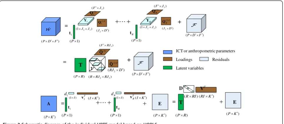
3 Multi-linear personalization modeling by HOPLS
When the individual core tensor and a few key parame-ters are obtained, a multi-linear HRTF personalization model can be learned by HOPLS regression. HOPLS is a generalized multi-linear regression model with the aim to predict a tensor from a tensor through projecting the data onto the latent space and performing regression on corresponding latent variables [41]. Moreover, it is par-ticularly suitable for small sample sizes [42]. HOPLS re-gression is used to explore the multi-linear subspace approximation for both the selected parameters and the HRTF tensor. It is employed to learn the relation be-tween the parameter matrix and the individual core tensor. The complexity of the regression model is con-trolled by the hyperparameters which are the numbers of orthogonal loadings denoted byJ2,J3,Iand latent vec-tors denoted byRin Figure 3. Figure 3 shows the frame-work of a joint subspace approximation for the ICT and the anthropometric parameters by the HOPLS model. After the regression model is constructed from training data, the individual HRTFs for a new subject can be pre-dicted by his anthropometric measurements.
Consider a second-order tensor A∈ℝPK′ containing the selected parameters and a third-order tensor W~ ∈
[24,43]. Here, based on the property, do a high-order ex-tension to find common latent variables for explaining the covariance betweenAand W~ , as illustrated in Figure 3. The mathematical model can be expressed as [41,42]
~
the latent vector tr on the mode of the sound direction
and the frequency, respectively; similarly, vr∈ℝK
′I
I≤K′
is the loading vector of the parameter matrixA, andFandEare the residuals. Use the rank-(1,J2,J3)
de-composition of the individual core tensor W~ to get the
core tensorYr∈ℝ1J22J3 corresponding to therth latent
vector. dr∈ℝ1 ×Iis the core of the anthropometric
par-ameter tensor by the rank-(1,I) decomposition. The
model in (10) is boiled down to a concise form as
~
block-diagonal matrix D∈ℝR×RI, direction loading
matrix Qð Þ2 ¼ Qð Þ12;Q
the anthropometric parameter loading matrix V¼½v1;
v2;⋯;vR∈ℝK
′RI
.
Observing Figure 3, how to chooseRand estimate the loading matrices from W~ andAis the key optimization of the multi-linear subspace regression for individual HRTF customization. There are two different ways for extracting the latent variables: sequential and simultan-eous methods. We choose to obtain the latent vectors in sequence since it provides better performance [42]. If the first latent vector is obtained, the other latent vectors can be estimated by the deflation of W~ andA. There-fore, we firstly find the latent vector t1 and the corre-sponding loading matrices Qð Þ1mðm¼2;3Þ and v1. The subscriptris omitted to simplify the notations in the fol-lowing discussions. The whole optimization is based on the strategy for the simultaneous minimization of the Frobenius norm of residuals F and E, while keeping a common latent vectort. Assume thatQ(2),Q(3), v, andt are given; then, the cores in (10) can be calculated as
Y¼W~ 1tT2Qð Þ2T3Qð Þ3T d¼A1tT2vT
ð12Þ
In [42], minimization of the Frobenius norm of the re-siduals F and E under the orthonormality constraint is converted to maximize a cross-covariance tensor. Zhao et al. defined a cross-covariance tensor of independent variables and dependent variables. Then, the optimization problem for loading matrices can be finally formulated as
max
where C¼ covA;W~ ∈ℝK′D′F′ is a 1-mode cross-covariance tensor [41]. We try to find a rank-(I, J2, J3)
tensor decomposition of C by employing HOSVD [34].
When the loading matrices of the parameters and the
in-dividual core tensor are estimated, the latent vector t
should explain the variance of the anthropometric pa-rameters as much as possible estimated by
t¼ arg min
t kA−D;t;vk
2
F ð14Þ
When the latent vector t is fixed, the cores Y and d are obtained by (12).
Once the latent vectors and loading matrices are esti-mated, the prediction of the individual core tensor for a new subject using the corresponding anthropometric measurementsanewcan be predicted as
Tnew ¼anewVDþ
In the section, the performance of the proposed method is measured by objective evaluation and subjective sound localization based on a large number of HRTF measure-ments. The Center for Image Processing and Integrated Computing (CIPIC) database provides high-spatial-resolution HRIR measurements of 45 different subjects. It contains measured HRIRs for both left and right ears at 1,250 sound directions (25 azimuths and 50 eleva-tions) [44]. The azimuths vary from−80° to 80°, and the elevations range from −45° to +230.625°. Moreover, 27 anthropometric parameters of 45 subjects are measured in the CIPIC database including 17 for the head and the torso from x1to x17and 10 for the pinna expressed by
d1−d8, θ1, and θ2[44]. The CIPIC database is used to evaluate the performance of our proposed regression model based on HOPLS.
4.1 Simulations of the data processing 4.1.1 HRTF tensor compaction
In the simulations, the HRTFs of the left ears are chosen to construct the model. The HRIRs in CIPIC of each sub-ject are transformed into HRTFs by a 200-point FFT. Col-lect the HRTFs of random 30 subjects acting as the training samples denoted by a third-order tensor H∈
ℝP×D×F, where
Pis the number of subjects (30),Dis the number of the sound source elevations (50), andFis the frequency points (100). The other subjects are used for testing the model. When the high-dimensional HRTF ten-sor is acquired, an individual core tenten-sor W∈ℝPD′F′ can be extracted from the original data via HOSVD. The following discussions focus on how to determine the
dimensionsD′andF′of the ICT and the performance of the HRTF tensor subspace approximation:
1. The selections ofD′andF′depend on the energy
loss of the original HRTF tensor in each mode, respectively. The energy contained in the HRTF tensor is calculated by the squared Frobenius norm
ofH. It also equals the sum of the squaredm-mode
singular values [34] expressed by
H
corresponding to them-mode of the HRTF tensor.
The square of them-mode singular value is called
them-mode eigenvalue denoted byλð Þim. The
eigenvalue magnitudes and their cumulative
distributions are shown in Figure4. The loss of
energy with the selectedD′andF′is proportional to
the sum of the corresponding singular values of the
discarded singular vectors contained inU(m). The
ratios of the retained energy to the total energy for
different modes areEð Þratio2 ¼
than the originalDandF. The dimension reduction
of the original HRTF tensorH∈ℝP×D×Fbrings
corresponding compression ratio (CR) as
CR¼ DFP
DD′þFF′þD′F′P ð17Þ
According to Figure4, the numbers of singular
vectors are kept in each mode, and the different CRs
are shown in Table1. Similar amount of energy is
kept in each mode with the sameEratio, but the
dimension reduction of each mode is quite different. This indicates that the redundancy of these two modes is different. The eigenvalue cumulative
distributions in Figure4show different redundancy
between the frequency mode and the sound
direction mode, resulting in different selections ofD′
andF′. Although with the sameEratio, similar
amount of variations is kept in each mode, the amount of dimension reduction in the frequency
mode (80% for the azimuth−80°, 64% for the
azimuth 0°, and 64% for the azimuth 80°) is different from that in the sound direction mode (90%, 48%,
and 70% for those three azimuths−80°, 0°, and 80°,
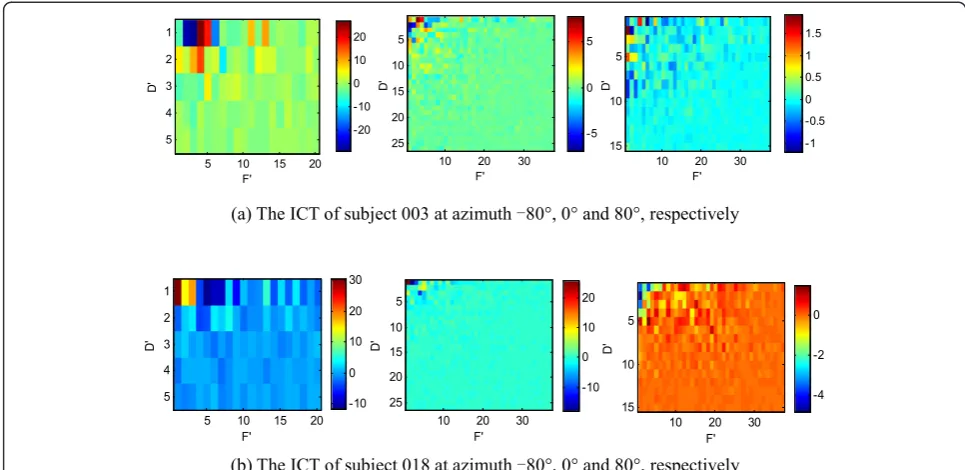
respectively). After dimension reduction ofH, the
HRTFs. Figure5shows the ICT for some subjects. It can be seen that the main energy of the ICT is concentrated in the upper left corner areas. 2. To measure the quantitative error of the
reconstruction using the basis functions and the
individual core tensor, the signal-to-distortion ratio (SDR) is defined in decibels as
SDRðp;θ;ϕÞ ¼10 lg
XF
f¼1
Hðp;θ;ϕ;fÞ
j j2
XF
f¼1
Hðp;θ;ϕ;fÞ−H^ðp;θ;ϕ;fÞ
2
ð18Þ
whereH(p,θ,ϕ,f) andH^ðp;θ;ϕ;fÞrepresent the
original and the reconstructed or predicted HRTF, respectively. The average of SDR (ASDR) defined as
Figure 4Eigenvalue magnitudes and their cumulative distributions for the HRTF tensor at different azimuths. (a)θ=−80°,(b)θ= 0°, and(c)θ= 80°.
Table 1 The selections ofD′andF′for three azimuths
Azimuth D′ F′ CR Eð Þratio2 Eð Þratio3
−80° 5 20 28.6
0° 26 37 4.4 0.98 0.98
ASDRðθ;ϕÞ ¼1 P
XP
p¼1
SDRðp;θ;ϕÞis used to measure
the mean performance for the reconstruction or prediction in the following discussions.
Figure 6a shows the ASDR for P= 30 subjects and the reconstruction with the correspondingD′andF′selection. In most cases, ASDR exceeds 20 dB. The average of ASDR over all the azimuths and elevations is 24.3 dB. The results imply that the reconstructed HRTFs can approximate the original HRTFs accurately via selecting appropriateD′and F′. For example, the reconstruction of the subject 003 at three sound directions (−80°, 0°), (0°, 0°), and (80°, 0°) are shown in Figure 6b,c,d compared to the original measured HRTFs. Moderate deviations between the original HRTFs and the reconstructed HRTFs occur at the frequencies of the spectral notches. These reconstruction errors imply that the information loss of the lower-dimensional HRTF tensor may affect the subsequent modeling.
4.1.2 Selecting anthropometric parameters
There are 27 parameters measured in the CIPIC data-base. The detailed definitions of these parameters can be referred in [44]. To avoid the loss of some important pa-rameters, a mass of correlation analyses are done be-tween all the parameters and the ICT instead of the original HRTFs. Three steps for selecting parameters are used in the following simulation:
1. In order to reduce the amount of computation and make correlation analyses more effectively, it is
desirable to sample the upper left corner areas of the ICT for correlation analyses. In this procedure, the
compacted ICT denoted byW~ c∈ℝPD
″F″
D″<D′
and F″<F′Þ is reshaped to a matrixW~c∈ℝPD
″F″ ð Þ.
Then, the absolute values of Pearson correlation coefficients are calculated and stored in a matrix
RW~cA∈ℝ27ðD″F″Þ. There are 25 compacted ICTs
corresponding to 25 azimuths, so 25 correlation analyses are constructed for the different azimuths. The significance of all the anthropometric parameters on the HRTFs can be shown by the correlation coefficient matrices with elements larger than 0.35
and plotted in Figure7. The results in Figure7show
that all the anthropometric measurements affect the HRTFs with different levels. It is necessary to delete
unimportant parameters. After 25 correlation
analyses, 22 parameters shown more important to the HRTFs are reserved for the next selection step. The
parameters x2, x4, x5, x7, and d2 have the weak
correlation with the HRTFs and they are deleted in this step.
2. After the correlation analyses, we model the intrinsic geometric structure of the reserved parameter space by the nearest neighbor graph.
These reserved parameters (x1,x3,x6,x8−x17,d1,
d3−d8,θ1,θ2) are arranged to three different classes
shown in Table2. Combining (8) and the graph, each
parameter is evaluated by a Laplacian score. These parameters of each class are arranged by their corresponding scores in an ascending sequence. By this means, 17 parameters are reserved as the results
Figure 7Correlation coefficients between the compacted ICT and the anthropometric parameters.
of the Laplacian score procedure. They arex3,x6,x9−
x15,x17,d1,d3,d4,d6−d8, andθ1with the Laplacian
score less than 0.4.
3. The selected parameters are fed into the training of the individual HRTF modeling by HOPLS. The last step performs the correlation analysis among the reserved parameters. Similarly in order to show the dependent relation among those parameters, the
gray image in Figure8presents the correlation
coefficients of the reserved parameters larger than
0.5. From Figure8,x6,x9,x12,x14, andx17have
strong correlation with others and are deleted. Thus, the parametersx3,x10,x11,x13,x15,d1,d3,d4,d6,d7,
d8, andθ1are selected as the final necessary
measurements for the individual HRTF prediction. All the final reserved parameters are selected by the procedures of the correlation analysis and the Laplacian score. We select these 12 parameters as the key parameters. However, the significance of each selected parameter on the HRTFs is still not clear. Since measurements of the anthropometric parameters need special instruments, we cannot implement the anthropometric measurements at present.
4.2 Objective evaluation and subjective localization experiment
Through the simulations in Section 4.1, we can obtain the individual core tensor and key anthropometric parameters.
The goal of our proposed HRTF personalization is to model the multi-linear relation between the key parame-ters and the individual core tensor. In this section, the ex-periments are implemented to evaluate the feasibility of the proposed individual HRTF customization by objective evaluation and subjective perception. It is important to se-lect the appropriate hyperparameters for preventing over-fitting and controlling the complexity of the HRTF estimation model.
4.2.1 Selecting the numbers of loadings and latent vectors for the individual HRTF prediction
The different selections for the numbers of loadings and latent vectors can control the personalization model complexity and improve the predicting performance. In order to simplify the selection, we defineJ2=J3=I=λ.λ andRare chosen based on cross-validation [43]. The re-sults of the optimal hyperparameters are shown in Table 3.
The optimalRandλof five predicted subjects at three azimuths are different. These optimal R and λ bring good predicted performance. The ASDR is larger than 12.46 dB, but lower ASDR is obtained by other selec-tions of R and λ. This implies that the performance of the individual HRTF prediction model can be adjusted by these two hyperparameters.
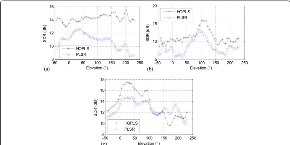
Compared with the PLSR method, the same 12 se-lected parameters are treated as the inputs and the ICT unfolded in 1-mode as the output. The optimal number of the latent variables in PLSR for the individual HRTF linear model is also chosen by cross-validation. The SDRs of the individual HRTF prediction for subject 124 at all the measured elevations of three different azimuths are shown in Figure 9. It can be seen that the proposed HRTF model has achieved larger SDRs than the PLSR method in all the elevations at azimuth−80° and 0°, ex-cluding the high elevations of azimuth 80°. The complex Table 2 Reserved parameters arranged by Laplacian
scores in an ascending order
Class Reserved anthropometric parameter
Class 1 (head and torso) x17,x15,x12,x6,x14,x9,x13,x11,x3,x10,x8,x16,x1
Class 2 (pinna) d3,d8,d4,d7,d1,d6,d5
Class 3 (pinna angle) θ1,θ2
property of the measured HRTFs for the contralateral ear especially at the rear directions near the horizontal plane leads to predict the individual HRTFs more diffi-cultly. The performance for predicting the individual HRTFs by HOPLS model is much better than that of the PLSR method especially for the sound directions
ipsilateral to the concerned ear. In Figure 10, the dis-crepancy between the original HRTFs and the individual HRTFs may be caused by the information loss in the di-mension reduction for the HRTF tensor and the inher-ent defect of the HOPLS model. In general, the predicted HRTFs can approximate the measured HRTFs based on the HOPLS method more accurately than the predicted HRTFs by PLSR.
4.2.2 Subjective localization experiment
The desirable individual HRTF modeling provides the accurate sound localization by the predicted HRTFs. The purpose of the subjective hearing experiment in this section is to compare the sound localization perform-ance of the original HRTFs and the predicted HRTFs. Subjective tests, using five pink noises repeated five times, with 0.5-s silence between each repetition are constructed by headphone listening binaural signals. The used pink noises have 22.05-kHz bandwidth and 44.1-kHz sample ratio. Five test subjects participate in the subjective listening experiment with five test stimuli. The five test stimuli are pink noise samples of duration 1 s with 50 ms onset and offset time [45]. Each pink noise sample is rendered using the predicted HRTFs as well as the measured ones at randomly chosen azimuths in the horizontal plane. Then, each rendering testing stimulus is played back through a headphone. The par-ticipating subjects are asked to mark the level of sound localization using the grades in Table 4. Figure 11 shows the results of the listening tests with the virtual sounds Table 3 The selected numbers of latent vectors and
loadings of HOPLS
Azimuth Subject HOPLS
R λ
−80° 003 1 1
033 4 1
124 5 4
134 4 2
153 3 5
0° 003 1 3
033 3 1
124 10 3
134 2 1
153 1 7
80° 003 1 3
033 7 5
124 10 7
134 4 3
153 1 9
by convolving the stimuli with the predicted HRTFs and the measured HRTFs of the subjects 003, 033, 124, 134, and 153. For the sound localization, the predicted HRTFs are approximate to the original HRTFs.
5 Conclusions
High-dimensional HRTFs and redundant anthropomet-ric parameters greatly affect the individual HRTF customization. We construct a multi-linear regression model between the HRTFs and the anthropometric pa-rameters. The individual core tensor as the output vari-able of the regression model is firstly extracted from the measured HRTFs. Then, the key parameters are selected as the input variables of the multi-linear model based on the individual core tensor. The appropriate hyperpara-meter selection can achieve good prediction perform-ance for the multi-linear model. Experimental results demonstrate the better performance for predicting the
individual HRTFs in comparison to the PLSR method especially for the sound directions ipsilateral to the con-cerned ear. The listening tests show that the predicted HRTFs are approximate to the original ones for the sound localization. The performance of the individual HRTF prediction is relatively not good in the region of the high elevations to the contralateral ear. In our future work, we will further implement the anthropometric measurements to predict the individual HRTFs and focus on the improvement of the prediction perform-ance of the contralateral HRTF personalization. At the same time, the non-linear methods for the HRTF tensor estimation will be our future task based on the current work.
Figure 10The individual HRTF prediction by HOPLS and PLSR compared with original HRTFs.
Table 4 Localization impairment scale in the subjective tests
Grade Localization similarity
1 Very different
2 Slightly different
3 Slightly similar
4 Very similar
Competing interests
The authors declare that they have no competing interests.
Acknowledgements
The authors would like to thank the editor and anonymous reviewers for their valuable comments. This work was supported by the National Natural Science Foundation (61001160) and Innovation Program of Shanghai Municipal Education Commission (12YZ023) of China.
Received: 31 August 2013 Accepted: 3 April 2014 Published: 3 May 2014
References
1. NA Gumerov, R Duraiswami, ZH Tang, Numerical study of the influence of the torso on the HRTF, inIEEE International Conference on Acoustics, Speech, and Signal Processing (ICASSP), vol. 2 (Orlando, 2002), pp. II1965–1968 2. NA Gumerov, AE O'Donovan, R Duraiswami, DN Zotkin, Computation of
head-related transfer function via the fast multipole accelerated boundary element method and its spherical harmonic representation. J. Acoust. Soc. Am.127(1), 370–386 (2010)
3. Y Kahana, PA Nelson, Boundary element simulations of the transfer function of human heads and baffled pinnae using accurate geometric models. J. Sound Vib.119(5), 552–579 (2007)
4. V Algazi, R Duda, R Duraiswami, N Gumerov, Z Tang, Approximating the head-related transfer function using simple geometric models of the head and torso. J. Acoust. Soc. Am.112(5), 2053–2064 (2002)
5. S Xu, Z Li, L Zeng, G Salvendy, A study of morphological influence on head-related transfer functions, inIEEE International Conference on Industrial Engineering and Engineering Management, Singapore, 2007, pp. 472–476 6. J Fels, M Vorlander, Anthropometric parameters influencing head-related
transfer functions. Acta Acustica united with Acustica95(2), 331–342 (2009) 7. M Rothbucher, T Habigt, JL Habigt, T Riedmaier, K Diepold, Measuring
anthropometric data for HRTF personalization, inProcessing of the 6th International Conference on Signal-Image Technology and Internet-Based Systems, Kuala Lumpur, 2010, pp. 102–106
8. M Zhang, RA Kennedy, TD Abhayapala, W Zhang, Statistical method to identify key anthropometric parameters in HRTF individualization, in2011 Joint Workshop on Hands-Free Speech Communication and Microphone Arrays, HSCMA'11(Edinburgh, 2011), pp. 213–218
9. DN Zotkin, J Hwang, R Duraswami, LS Davis, HRTF personalization using anthropometric measurements, inIEEE ASSP WASPAA'2003, New Paltz, 2003, pp. 157–160
10. XY Zeng, SG Wang, LP Gao, A hybrid algorithm for selecting head-related transfer function based on similarity of anthropometric structures. J. Sound Vib.329(19), 4093–4105 (2010)
11. N Inoue, T Kimura, T Nishino, K Itou, K Takeda, Evaluation of HRTFs estimated using physical features. Acoust. Sci. Technol.26(5), 453–455 (2005) 12. HM Hu, L Zhou, J Zhang, H Ma, ZY Wu, Head related transfer function
personalization based on multiple regression analysis, in IEEE International Conference on Computational Intelligence and Security. Guangzhou 2, 1829–1832 (2006)
13. S Xu, ZZ Li, G Salvendy, Improved method to individualize head-related transfer function using anthropometric measurements. Acoust. Sci. Technol. 29(6), 388–390 (2008)
14. K Matsui, A Akio, Estimation of individualized head-related transfer function based on principal component analysis. Acoust. Sci. Technol.30(5), 338–347 (2009) 15. S Hwang, YJ Park, YS Park, Modeling and customization of head-related transfer
functions using principal component analysis, inIEEE International Conference on Control, Automation and Systems(ICCAS)(Seoul, 2008), pp. 227–231 16. J Sodnik, A Umek, R Susnik, G Bobojevic, Representation of head related
transfer functions with principal component analysis, inProceedings of the Annual Conference of the Australian Acoustical Society, NSW, 2004, pp. 603–607 17. L Wang, FL Yin, Z Chen, HRTF compression via principal components
analysis and vector quantization. IEICE Electron Express5(9), 321–325 (2008) 18. L Wang, FL Yin, Z Chen, Head-related transfer function interpolation
through multivariate polynomial fitting of principal component weights. Acoust. Sci. Technol.30(6), 395–403 (2009)
19. BS Xie, Recovery of individual head-related transfer functions from a small set of measurements. J. Acoust. Soc. Am.132(1), 282–294 (2012)
20. DJ Kistler, FL Wightman, A model of head-related transfer functions based on principal components analysis and minimum-phase reconstruction. J. Acoust. Soc. Am.91(3), 1637–1647 (1992)
21. G Grindlay, MAO Vasilescu,A multilinear (tensor) framework for HRTF analysis and synthesis. IEEE International Conference on Acoustics, Speech and Signal Processing (ICASSP), vol. 1 (Honolulu, 2007), pp. I161–164
22. M Rothbucher, M Durkovic, H Shen, K Diepold, HRTF customization using multiway array analysis, inEUSIPCO'2010(Denmark, 2010), pp. 229–233 23. ZW Chen, GZ Yu, BS Xie, SQ Guan, Calculation and analysis of near-field
head-related transfer functions from a simplified head-neck-torso model. Chin. Phys. Lett.29(3), 034302 (2012)
24. HM Hu, L Zhou, H Ma, ZY Wu, Head-related transfer function personalization based on partial least square regression. J. Electron. Inform. Technol. 30(1), 154–158 (2008)
25. HM Hu, L Zhou, H Ma, ZY Wu, HRTF personalization based on artificial neural network in individual virtual auditory space. J. Appl. Acoust. 69(2), 163–172 (2008)
26. S Xu, ZZ Li, S Gavriel, Individual head-related transfer functions based on population grouping. J. Acoust. Soc. Am.124(5), 2708–2710 (2008) 27. W Hugeng, D Gunawan, Improved method for individualization of
head-related transfer functions on horizontal plane using reduced number of anthropometric measurements. J. Telecommun.2(2), 31–41 (2010) 28. T Nishino, N Inoue, K Takeda, F Itakura, Estimation of HRTFs on the
horizontal plane using physical features. Appl. Acoust.68(8), 897–908 (2007) 29. T Nishino, Y Nakai, K Takeda, F Itakura, Estimating head related transfer
function using multiple regression analysis. IEICE Trans. A84, 260–268 (2001) 30. QH Huang, Y Fang, Modeling personalized head-related impulse response using
support vector regression. J Shanghai Univ (English edition)13, 428–432 (2009) 31. QH Huang, QL Zhuang, HRIR personalisation using support vector regression
in independent feature space. Electron. Lett.45(19), 1002–1003 (2009) 32. L Li, QH Huang, HRTF personalization modeling based on RBF neural
network, inIEEE International Conference on Acoustics Speech and Signal Processing (ICASSP), Vancouver, 2013), pp. 3707–3710
33. M Rothbucher, H Shen, K Diepold, Dimensionality reduction in HRTF by using multiway array analysis, inHuman Centered Robot Systems(Springer, Berlin, 2009), pp. 103–110
34. LD Lathauwer, LD Moor, J Vandewalle, A multilinear singular value decomposition. SIAM J Matrix Anal Appl21(4), 1253–1278 (2000) 35. G Bergqvist, EG Larsson, The higher-order singular value decomposition:
theory and an application [lecture notes]. IEEE Signal Process. Mag. 27(3), 151–154 (2010)
36. TG Kolda, BW Bader, Tensor decompositions and applications. SIAM Rev. 51(3), 455–500 (2009)
37. BS Xie, XL Zhong, D Rao, ZQ Liang, Head-related transfer function database and its analyses. Sci. China, Ser. G50, 267–280 (2007)
38. LD Lathauwer, BD Moor, J Vandewalle, On the best rank-1 and rank-(R1, R2,…, RN) approximation of higher-order tensors. SIAM J Matrix Appl21(4), 1324–1342 (2000) 39. N Gupta, A Barreto, M Joshi, JC Agudelo, HRTF database at FIU DSP Lab, in
IEEE International Conference on Acoustic Speech and Signal Processing (ICASSP), Dallas, 2010), pp. 169–172
40. X He, D Cai, N Partha, Laplacian score for feature selection, inProceedings of Advances in Neural Information Processing Systems(Vancouver, 2005), pp. 507–514 41. QB Zhao, CF Caiafa, DP Mandic, L Zhang, T Ball, A Schulze-Bonhage, A
Cichocki, Multilinear subspace regression: an orthogonal tensor decomposition approach, inAdvances in Neural Information Processing Systems 24 (NIPS)(Granada, 2011), pp. 1269–1277
42. QB Zhao, CF Caiafa, DP Mandic, ZC Chao, Y Nagasaka, N Fujii, L Zhang, A Cichocki, Higher-order partial least squares (HOPLS): a generalized multi-linear regression method. IEEE Trans Pattern Anal Mach Intell35(7), 1660–1673 (2013) 43. HW Wang,Partial Least Square Regression-Method and Application(National
Defense Industry Press, Beijing, 2009), pp. 150–170
44. CIPIC HRTF database files, release 1.0. http://interface.cipic.ucdavis.edu/. Accessed 28 July 2012
45. PS Chanda, S Park, TI Kang, A binaural synthesis with multiple sound sources based on spatial features of head-related transfer functions, inIEEE IJCNN'06(Vancouver, 2006), pp. 1726–1730
doi:10.1186/1687-6180-2014-58