Preamble based frequency domain joint CFO and STO estimation for OQAM based filter bank multicarrier

R E S E A R C H

Open Access

Preamble-based frequency-domain joint CFO

and STO estimation for OQAM-based filter

bank multicarrier

Stijn Van Caekenberghe

, André Bourdoux

, Liesbet Van der Perre

and Jérôme Louveaux

Abstract

Filter bank multicarrier systems, similarly to orthogonal frequency division multiplexing (OFDM), are very sensitive to carrier frequency offset (CFO) and symbol timing offset (STO). In this paper, a low-complexity preamble-based joint CFO and STO technique is presented. It is based on a relatively long preamble in order to improve the CFO estimation performance as well as avoid interference coming from the data following this preamble. After CFO and STO

correction, the preamble can be reused to estimate the channel. Unlike most current techniques, the CFO and STO estimation occurs in the frequency domain. This allows for a low-complexity estimation with respect to time-domain techniques and, as will be shown by simulations, provide even better performance in a reasonable range. The drawback however is that the estimation range is shorter. Specifically, for large STOs (and to a smaller extent large CFOs), the performance decreases below time-domain estimations. Two versions of the STO estimation technique will be presented, the second one being an approximation of the first one, making it less complex yet also less precise. The performance is assessed by means of computer simulations, testing for both large and small STOs, and compared with existing techniques.

Keywords: Preamble-based estimation; Carrier frequency offset; Symbol timing offset; Filter bank multicarrier

1 Introduction

Filter bank multicarrier (FBMC) is a family of multicarrier modulation techniques that use discrete Fourier trans-form (DFT)-modulated filter bank in order to obtain a better spectral containment than the traditional orthogo-nal frequency division multiplexing (OFDM). There exists different versions of FBMC such as filtered multitone (FMT) and offset QAM (FBMC/OQAM). We focus on the latter in this paper. The FBMC/OQAM offers, at the expense of an increased complexity, several advantages over OFDM. The first one is the gain in spectral effi-ciency related to the removal of the cyclic extension. But the major advantage is the possibility to have several coex-isting systems with very little guard bands, which is a very desirable property in wireless communications where spectrum is expensive and should be used as efficiently as possible. For this reason, FBMC has been strongly

*Correspondence: [email protected]

3Université catholique de Louvain, Place du Levant, 2, Louvain-la-Neuve B-1348, Belgium

Full list of author information is available at the end of the article

considered for cognitive applications recently [1] as well as several other applications such as professional mobile radio (PMR) or 5G mobile networks. Just like OFDM, FBMC is highly sensitive to carrier frequency offset (CFO) and symbol timing offset (STO). A good estimation and correction technique is therefore essential.

There has been a lot of literature on CFO and STO esti-mation for OFDM, but most of these techniques cannot be directly applied to FBMC/OQAM due to the removal of the cyclic extension and due to the particular struc-ture of the OQAM. Hence, a good amount of research has been devoted recently to specific techniques for the synchronization in FBMC/OQAM. The literature focused on blind estimation methods initially. In [2], a blind joint CFO and STO estimation has been presented based on the cyclostationarity of the FBMC/OQAM signal. In [3], the CFO estimation is further improved by using the conjugate second-order cyclostationarity statistics. Then, a frequency-domain implementation is proposed in [4]. In [5], a blind CFO estimator is obtained based on the

maximum likelihood (ML) principle for low signal-to-noise ratio (SNR). In [6], a blind closed-loop method is proposed for the tracking of the STO based on the ML estimation, with several approximation to obtain a computationally efficient algorithm. More recently, pilot-based (or preamble-pilot-based) synchronization has received more attention. In [7], a periodic preamble is consid-ered, and both STO and CFO estimators are designed based on a least-square (LS) approach. This is a time-domain approach and exhibits a stable performance inde-pendently of the actual STO, making it very well suited as a coarse alignment algorithm. It also provides good robustness against multipath channels but has rather high complexity. In [8], the same authors develop a joint STO and CFO estimator for short nonperiodic preamble based on the ML principle. A closed-form approximate expres-sion of the CFO estimation is presented that provides accurate performance for moderate values. Another time-domain technique that should be mentioned is presented in [9] for FMT. And in [10], LS-based CFO and STO estimation is investigated for a short preamble, designed specifically for low latency and simplified channel estima-tion. In [11], a CFO estimation is derived for scattered pilots based on the ML principle and taking into account mobility as well as channel dispersion. In [12] and [13], a frequency-domain approach is considered for various pilot schemes inspired from WiMAX but using the auxil-iary pilots [14] or pair of pilots [15] (POP) principle. Due to this frequency-domain approach, it leads to lower com-plexity algorithms but the performance suffers for large values of the CFO and/or STO and it is more suited to a tracking scenario or for refining the estimation.

In this paper, we are interested in low-complexity synchronization methods using closed-form expressions while still providing accurate estimations. Because it is easier to implement in many system architectures, we focus on a frequency-domain implementation, i.e., work-ing with the demodulated symbols after the receiver’s analysis filter bank. As opposed to the literature described above, we do not focus on a particularly short pream-ble [8,10] or scattered pilots [11,13], but we instead consider a specific preamble designed to alleviate the interference structure of the OQAM modulation without requiring the use of auxiliary pilots or POP. This pream-ble is relatively long and might not be appropriate for low-latency applications but is able to provide efficient synchronization. In particular, the length helps improving the CFO accuracy. For this preamble, we design a spe-cific STO estimation and also show that accurate CFO can be obtained with a simple adaptation of a known technique. As with other frequency-domain methods, the best performance is obtained for offsets (both CFO and STO) which are not too large. So, it might be necessary to perform a very low complexity coarse estimation before

applying the filter bank, in order to ensure that the STO is within reasonable range. Especially large STOs degrade the performance of this estimation technique. This will be illustrated in the simulation results.

In this paper, we will focus on the OQAM flavor of FBMC. The OQAM modulation sends symbols on the real and imaginary part alternatively with T/2 spacing. Because of this structure, it is frequent to perform frac-tionally spaced equalization at the receiver, using T/2 spacing at the output of the analysis filter bank [16]. The STO estimation method proposed here will be using this double sampling rate at the receiver. Other flavors of FBMC, such as FMT, do not necessarily have this double sampling rate. The method can be generalized to those cases as well, but it requires that the double sampling rate be introduced at the receiver, at least for the duration of the preamble.

The rest of the paper is organized as follows. In Section 2, the FBMC/OQAM system is described. In Section 3, the preamble is introduced, and we explain how the STO and CFO can be estimated using this received preamble. The simulation results of the CFO and STO estimation will be presented in Section 4, and the perfor-mance of the proposed method is compared with the LS approach of [7].

2 FBMC/OQAM system model

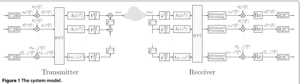
Consider an FBMC/OQAM system withMsubcarriers, as shown in Figure 1. At the input of the transmitter, QAM symbols are converted to OQAM, which is represented by theC2Rblock on the figure. The QAM symbols have a durationT, with 1/Tbeing the subcarrier spacing. The sampling rate isM/Tat the output of the transmitter. For the description of the FBMC/OQAM, we use a formalism based on real symbols similar to the one used in [1]. The purely real OQAM symbol for subcarrier k at sampling instantnM/2 will be denoted byd_kR[nM/2]. The alterna-tively real and imaginary symbols to be transmitted are denoted as (see Figure 1)

dk

The prototype filter is denoted bya[m]. The output of the transmitters[m] can be written as

s[m]=

Figure 1The system model.

in Figure 1). This filter is used in a DFT-modulated fil-ter bank. The length of the prototype filfil-ter isKM, with K being the overlapping factor and M the number of subcarriers. In the frequency domain, neighboring sub-channels will overlap, and this causes interference. When we send an impulse on one subcarrier, contributions will be received on the neighboring subcarriers. Other subcar-riers only have negligible contributions. By using OQAM, this interference can easily be removed.

The received symbols after the analysis receive filter bank are denoted byxk[nM/2] for subcarrier k at sam-pling instantnM/2. After multiplication withθ_k∗[nM/2] (the complex conjugate ofθk[nM/2]), the real part is taken to recover the estimation of the initial real symbol. The obtained value is denoted byxR_k[nM/2]. Now, for timing estimation purposes, it is worthwhile to look atxk[m] in between the symbol instants or, in other words, neglecting the downsampling that occurs in the receiver’s synthesis filter bank. For anidealchannel, it can be written as

x_k[m] =

is the convolution of the prototype filters on subcarriersk andk(we use∗to denote a convolution). The second and third terms of (4) are the interference terms from neigh-boring subcarriers. Non-neighneigh-boring subcarriers have

negligible interference, thanks to the spectral contain-ment of the prototype, i.e.,aˆk,k+w[m]≈ ˆak+w,k[m]≈0 for integerw>1.

When taking into account the influence of CFOφ, STO

δ, and channel impulse responsec[m], the received signal ˜

s[m] can be written as

˜

s[m]=(s[m+δ]∗c[m])ej2πφ(m+δ)/M+n[m] , (6)

wheren[m] is the additive noise.

3 Joint CFO and STO estimation

The preamble suggested in this paper has a duration of four multicarrier symbols, i.e., 4T. Thenth preamble sym-bol on thekth subcarrier will be denoted bypk[nM/2] in the transmitter and the corresponding received samples byyk[m] in the receiver (similarly todk[m] andxk[m] for data symbols). The preamble can now be defined as

pk

The received preamble is processed right after the IFFT in the receiver, i.e., the subchannel processing blocks in Figure 1. According to (4), and assuming that the channel is approximately flat inside each subcarrier, the received symbols on subcarrier k (denoted by yk[m] instead of xk[m] when they correspond to the preamble) can be written as is the channel coefficient on subcarrierk. The channel is assumed to be constant on the duration of the four pream-ble symbols. We assume additive white Gaussian noise (AWGN) with varianceσ2

n. In case of CFOφand STOδ,

The STO estimator is based on the observation of the amplitudeof the received preamble symbols|yk[nM/2]| on all subcarriers k for the first part of the preamble n = 0, 1,. . ., 4 (the second partn = 5, 6, 7 is potentially corrupted by intersymbol interference from the data sym-bols that follow). Note that even though the preamble is nonzero only forn = 0 andn = 4, all samples contain some information for the purpose of timing estimation, and we can thus take advantage of the structure of OQAM working atT/2 to utilize the overall information here.

In order to understand the derivation of the STO esti-mator below, it is interesting to investigate theamplitude of the received preamble |yk[m]| on the different sub-carriersk for all sample instantsm. As an example, the amplitude |y0[m]| for subcarrierk = 0 is illustrated in

Figure 2 for an ideal channel in the absence of noise. Note the raised cosine filter shape caused by the root raised cosine prototype filter in the filter bank. The STO can be estimated by looking at the difference in amplitude between the received preamble symbols |yk[M/2]| and |yk[3M/2]|, similarly to the way it is done for early-late tracking, and as it is illustrated in Figure 2. For instance, when the STO increases, the amplitude of yk[M/2] will decrease while the amplitude ofyk[3M/2] will increase. To cope with frequency selective channels and to increase

the precision,|yk[M/2]|and|yk[3M/2]|are combined for all even subcarriersk.

The estimation method proposed here is using four amplitude samples per subcarrier: |y_k[0]|, |y_k[M/2]|, |yk[3M/2]|, and |yk[2M]|. It is based on the early-late principle [18] and can be derived by using a few approxi-mations and assumptions:

• The four amplitude samples are modeled as linearly dependent on the STO, using a first-order

approximation aroundδ=0. In particular, the samples|yk[0]|and|yk[2M]|, which have a zero slope aroundδ=0(see Figure 2), are assumed to be roughly independent of the STO. This approximation is obviously valid only for small STO and makes the method less accurate at high STO. This effect can be partly compensated by using theoverall reference function as defined and explained below, which provides a reasonable range to the method. • The noise variance is assumed to be constant on all

subcarriers (before applying any equalization coefficient). This is usually a valid assumption. • The combination across all subcarriers is performed

using maximum ratio combining (MRC), which requires knowledge of the channel coefficients amplitudes. To this end and based on the

approximation described above, the samples|yk[0]| and|yk[2M]|are used as estimations of the channel amplitudes.

• The channel coefficients are assumed to be constant on the duration of the preamble, which is the case for most applications.

The expression of the estimator is derived below. Based on the linear approximation described above, the ampli-tude sample|yk[0]|can be written as denotes the contribution of additive noise on the ampli-tude samples of interesta. Similarly,

|y_k[2M]| ≈√G|C_k| +n_k,4. (13)

−1000 −500 0 500 1000 1500 2000 0

0.1 0.2 0.3 0.4 0.5 0.6 0.7 0.8 0.9 1

m

amplitude

|y₀[m]|

|y₀[nM/2]| for δ = 0

|y

0[nM/2]| for δ = 20

n=0

n=1 n=3

n=4

Figure 2Amplitude of a received preamble fork=0withG=1.The time axis has a sampling rate ofM/T(withM=512 in this case), while the processed preamble symbolsy0[nM/2] (crosses in the figure) have a rate of 2/T. If an STOδis applied, the amplitude ofy0[nM/2] will be different (circles in the figure).

whereSk,φis the slope of the amplitude with respect to the

STO

Sk,φ = −

∂aˆk,k,φ,δ[M/2]+ ˆak,k,φ,δ[−3M/2]

∂δ

_δ=

0

.

(15)

Similarly,

|yk[3M/2]| ≈ √

G|Ck|

|ˆak,k,φ,δ=0[3M/2]

+ ˆak,k,φ,δ=0[−M/2]| +Sk,φδ

+n_k,3. (16)

Due to the symmetry of the prototype, it is easy to show that the slopes at M/2 and 3M/2 are exactly opposite to each other and that the linearization points at M/2 and 3M/2 have the same amplitude: |ˆak,k,φ,δ[M/2]+ ˆak,k,φ,δ[−3M/2]| = |ˆak,k,φ,δ=0[3M/2]+

ˆ

ak,k,φ,δ=0[−M/2]|. Hence, based on the linearization and

on the early-late principle, a first quantity proportional to the STO can easily be obtained from the samples at subcarrierk:

ˆ

δk = |yk[3M/2]| − |yk[M/2]| (17) = 2δSk,φ| ˆCk|

√

G+(nk,3−nk,1). (18)

Now, one such quantity can be obtained for each sub-carrierk. All theses quantities can then be combined using MRC to form an estimate of the STO. It can be shown that for an ideal channel and for the prototype filter used here, the slopesSk,φare identical for all subcarriersk. Based on

this, assuming identical noise variances on all subcarriers

and optimizing the weights to minimize the estimation variance under the constraint of an unbiased estimator, it can be shown that the MRC weights corresponding to the different subcarriers must be proportional to| ˆCk|. Hence, the overall MRC estimate can be written as

ˆ

δ= 1

Anorm

M−1

k=0

| ˆCk|(|yk[3M/2]| − |yk[M/2]|) (19)

with some normalization coefficient Anorm. In practice,

the channel amplitudes are not yet available, so the values |yk[0]| and |yk[2M]| are used as estimates of the chan-nel amplitude inside each subcarrier. The estimation is then normalized in order to be independent of the chan-nel coefficient. Finally, only even subcarriers are taken into account as no symbols are sent on odd subcarriers in the chosen preamble. In the end, the estimation is based on the following quantity:

ˆ

z(δ,φ)= ˆy↑− ˆy↓ (20)

with

ˆ y↓=

M/2−1

k=0

|y2k[M/2]||y2k[0]|

M/2−1

k=0

|y2k[0]|2

and

ˆ y↑=

M/2−1

k=0

|y2k[3M/2]||y2k[2M]|

M/2−1

k=0

|y2k[2M]|2

. (22)

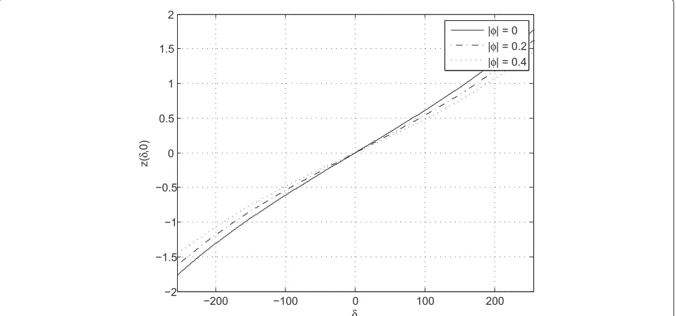
Note that this quantity is a function of both the STOδ and the CFOφ as emphasized in the notation. It is rep-resented in Figure 3 as a function of the STO when there is no CFO (φ = 0), for a prototype filter with overlap-ping factorK=4 and for an ideal channel in the absence of noise. It appears clearly that it is approximately linear on a significant range of STO values and can therefore be used efficiently to perform the STO estimation. In the-ory, the function can even be used if it is not linear, as long as it is a known one-to-one relationship with the true STO. In this paper, both methods are considered. We start with the more general one, assuming a known one-to-one relationship between the STO and the value of the quan-tity (20). In order to analyze this relationship, we define the so-calledreference function. This reference function will be denoted by z(δ,φ)and is defined as the value of ˆ

z(δ,φ)for an ideal channel and in the absence of noise (the effect of noise will be investigated in more detail in Section 3.1.3). In other words,ˆz(δ,φ)represents the actual measured value computed with (20) to (22), whilez(δ,φ) represents the theoretical value that would be obtained on an ideal channel and in the absence of noise. If a reason-able estimateφˆof the CFO has been obtained (for instance

using the technique explained in the next subsection), the STO can be estimated as

ˆ

δ=arg min|z( ,φ)ˆ − ˆz(δ,φ))| (23)

In the second part, we consider a linear approximation of the reference function which provides a simpler but less precise estimation.

3.1.1 General version

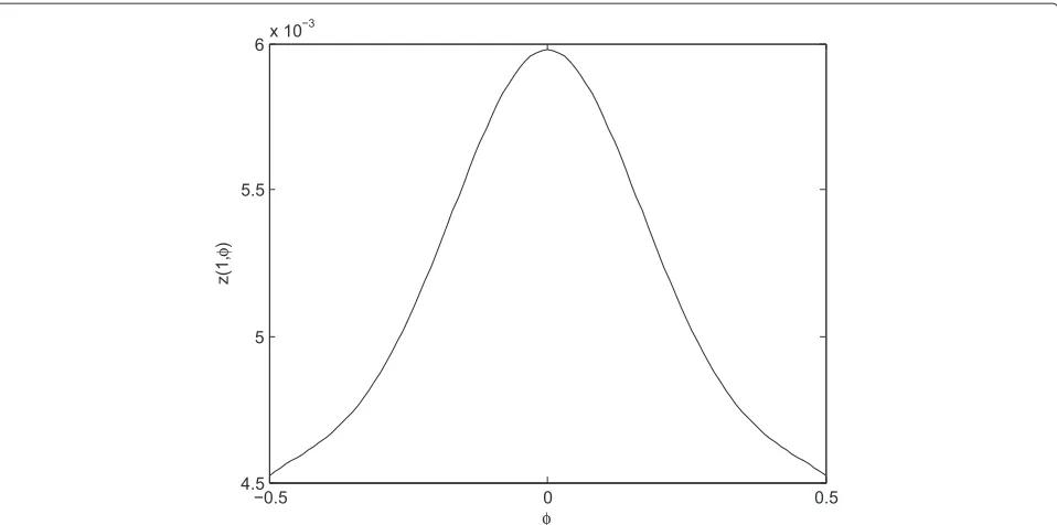
Let us first analyze the reference functionz(δ,φ). As pre-viously stated, this reference function is defined aszˆ(δ,φ) on an ideal channel and in the absence of noise. Figure 3 illustrates this reference functionz(δ,φ)for three values of the CFO. It is unbiased and exhibits a very good linear-ity except for large STO (close to±M/2). The slope of the curve however depends on the CFO. This is further illus-trated in Figure 4 which representsz(1,φ)as a function of the CFOφ. A larger slope is of course preferable as it makes the estimate less sensitive to additional noise. So, the estimation method performs better when the CFO is small although the difference is not very large, as can be seen in Figure 3.

The principle of the estimation, as described in (23) is to compute a reference function in advance and iden-tify which value of the STO corresponds to the observed value of the quantity (20). Note thatz(δ,φ)does not have to be recalculated for each estimation. It can be precal-culated and stored in memory. Therefore, in a practical implementation, the minimization of (23) does not require a long search over a large set of values; it simply corre-sponds to a look-up table. The estimation method is thus

−200 −100 0 100 200

−2 −1.5 −1 −0.5 0 0.5 1 1.5 2

z(

δ

,0)

δ

|φ| = 0 |φ| = 0.2 |φ| = 0.4

−0.5 0 0.5 4.5

5 5.5

6x 10

−3

φ

z(1,

φ

)

Figure 4The reference functionz₍1,_φ)in function of the CFO_φin the case of an STO_δ=1.The larger the CFO in absolute value, the smallerz(1,φ).

of low complexity; it amounts to the computation of one closed-form expression (20) followed by a look-up table. Regarding the memory needed, the STO is discrete, but the CFO is not. The reference function should be precal-culated for a number of CFOs and interpolated for the others. The larger that number, the more precise the ref-erence function (and hence the STO estimation) will be and the larger the memory usage as well. As can be seen in Figure 4,z(δ,φ)=z(δ,−φ)which can help reduce the memory usage.

3.1.2 Linear approximation

In order to reduce the memory usage even more, the reference function can be approximated linearly:

˜

z(δ,φ)=z(0,φ)+z(1,φ)δ (24)

It is clear from Figure 3 that this approximation is quite accurate for moderate values of the STO. For large STOs, the approximation error becomes more significant how-ever. Using this approximation, the complexity of the STO estimation reduces even further:

ˆ

δ= ˆy↑− ˆy↓−z

0,φˆ

z

1,φˆ

(25)

3.1.3 Effect of the noise

When AWGN is added to the channel, all the amplitude samples |yk[iM/2]| are corrupted by noise. Now, since the noise on the initial yk[iM/2] samples is Gaussian,

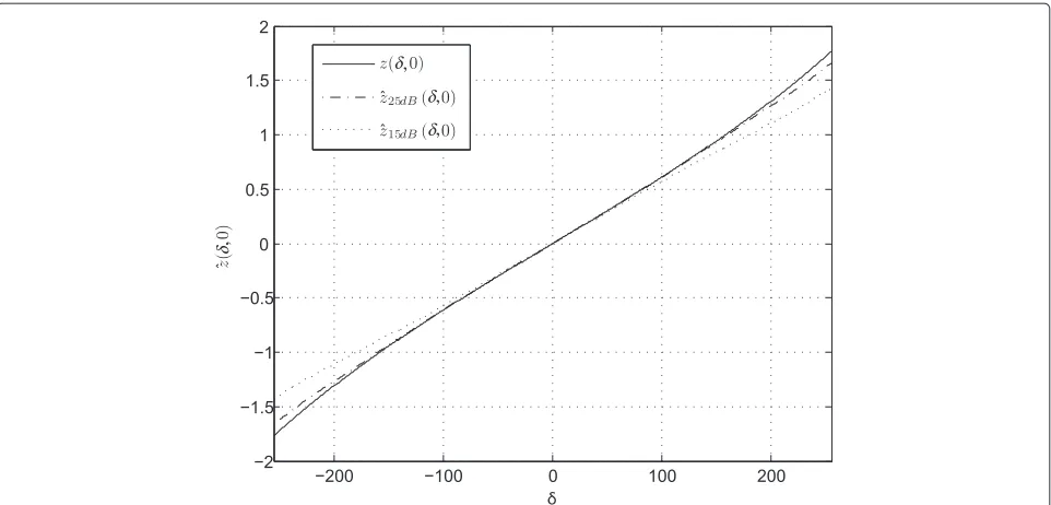
the probability density function of the amplitude sam-ples|yk[iM/2]|is a Rice distribution. In particular, it also means that the average effect of the noise isnotzero. On average, the respective contributions of the noise on y↓ andy↑donotcancel each other, and the estimateˆz(δ,φ) deviates from the reference functionz(δ,φ). The overall effect is illustrated in Figure 5 which represents the aver-age value of the estimateˆz(δ,φ)in the presence of noise as a function of the STOδand when the CFOφ=0. Two SNR cases (15 and 25 dB, respectively) are presented, and the result is compared to the reference functionz(δ,φ)in the absence of noise. Once again, the effect is negligible for small STOs and more significant at high STOs. This generates an estimation error that gets larger for higher STOs. However, it is interesting to observe that the aver-age effect of the noise at high (positive) STO is to decrease the estimatezˆ(δ,φ), which is the opposite of the nonlin-ear behavior of the reference functionz(δ,φ)that tends to deviate above the linear slope. The overall result is that the average estimatezˆ(δ,φ)exhibits an even better linear behavior than the reference functionz(δ,φ)as can be seen on Figure 5. In order to explain this, a complete analyti-cal derivation of the noise distribution forˆz(δ,φ)would be long and tedious, so we restrict ourselves to a qualitative justification which is provided in the Appendix.

3.1.4 Effect of the multipath channel

−200 −100 0 100 200 −2

−1.5 −1 −0.5 0 0.5 1 1.5 2

δ

ˆ

z

(0

)

z( 0) ˆ

z25dB( 0) ˆ

z15dB( 0)



  









Figure 5Effect of the noise on the reference function.The mean ofˆz(δ, 0)on a 25- and 15-dB AWGN channel, as well as the reference functionz(δ, 0).

anymore depending on the channel impulse response taps. The longer the channel, the larger the divergence with the reference functionz(δ,φ)can be.

To improve the estimation, it is possible to use some basic information about the channel. The idea is to assume some statistical channel model and try to take its effect into account in the reference function. A new reference function zmult(δ,φ) is used in that case, that is simply

replacingz(δ,φ)which was calculated for an ideal chan-nel. This new reference functionzmult(δ,φ)is defined as

the expectation ofˆz(δ,φ)in (20) in the absence of noise and averaged over the possible realizations of the chan-nels, according to the chosen model. In practice, it is difficult to obtain the true expectation; so, the practi-cal computation ofzmult(δ,φ)comes down to computing

it for a certain number of realizations and compute the average.

Just as previously, this new reference function is com-puted in advance without the knowledge of the true channel realization, but some channel model needs to be available. Obviously, the accuracy of the model has a direct impact on the performance of this method. Several results are presented below in the simulation section.

3.1.5 Complexity

Even though a detailed complexity analysis would depend on the chosen implementation, and hence is outside the scope of this paper, a few comments can be made on the issue of complexity. As mentioned above, the pro-posed method relies on a closed-form expression, and does not require a min or max search over a potentially

large number of candidates, which helps reduce the com-plexity significantly. The method also assumes that the frequency-domain samples of the preamble are available, so the method is for instance very well suited to an archi-tecture where the analysis filter bank is implemented separately and applies to all received symbols, including the preamble.

3.2 CFO estimation

The CFO estimation used here is a direct application of the one presented in [19] for OFDM. Similar CFO esti-mation methods have also been used for FBMC/OQAM systems in [12,13,20] although for different preamble schemes. The CFOφis estimated by looking at the phase difference between the received preamble symbolsyk[0] andyk[2M] on each even subcarrierk. The estimated CFO will be denoted byφˆ:

ˆ

φ= 1

4π∠ ⎛ ⎝M/2−1

k=0

y∗_2k[0]y2k[2M] ⎞

⎠ (26)

smaller than [−0.25, 0.25] and depends on the SNR of the channel.

To cope with this problem, a heuristic adjustment has been used. It is taking into account the sign of the phase difference betweenyk[M/2] andyk[3M/2]. This phase dif-ference will be denoted byφˆs. When the CFO is large and there is a risk of ambiguity,φˆsis taken into account. When the CFO is small on the other hand,φˆsis neglected since it is more susceptible to noise in this case thanφˆ. Hence, the estimated CFOφ˜is value was chosen to assure correct CFO estimation for CFOs in the range ofφ∈[−0.25, 0.25] even when the SNR is low. It is the result of a trade-off but does not come from any specific theoretical justification.

Note that in the method proposed here, the CFO is estimatedbeforethe STO. Hence, the CFO estimation is sensitive to the actual STO (as it could not be compen-sated yet). This is mainly due to the interference between the preamble symbols. For δ = 0, there is no interfer-ence from one preamble symbol to the other onyk[0] and y_k[2M]. However, when the STO increases, the interfer-ence increases which modifies the observed phases and degrades the CFO estimation.

4 Simulation results

To assess the performance of the CFO and STO estima-tion, the technique presented in this paper is compared with the LS technique of [7]. Note that this LS technique is a time-domain algorithm and hence corresponds to a different implementation architecture, with different con-straints on the complexity. It is however also a preamble-based technique, and it is an appropriate benchmark to evaluate the performance of the proposed method. The preamble used in [7] has a duration of 3T, so we have added a zero guard symbol of lengthTto reach the same total length 4Tas the preamble used in this paper, without

any impact on the estimation technique. Both pream-bles have been normalized for equal transmitted power. About 104 _{trials were performed under the following}

conditions:

• The number of subcarriers wasM=512. The overlapping factor of the prototype filter wasK=4 ([17]).

• The (normalized) CFO was uniformly distributed in φ ∈[−0.25, 0.25]. Notice that this is the maximum range that can be estimated correctly. In order to have a good estimation for CFOs on the edges of this range, the threshold to use the adjustment was set on | ˜φ| =0.15, as in (27).

• The STO was simulated in two ranges:

– STOδ ∈[−M/2,M/2]=[−256, 256] – STOδ ∈[−M/16,M/16] =[−32, 32]

• The multipath channel has been modeled to consist of 17 independent Rayleigh fading tapsh(l)with an exponentially decaying power delay profile.

Specifically,E[|h(l)|2]=Ce−l/4, where the constant Cis chosen for total unit energy16_l=0E[|h(l)|2]=1. The channel was different in each trial.

• The STO was estimated (with a granularity of one sample) using reference functionsz(δ,φ),zmult(δ,φ),

and their respective linear approximations. All of these reference functions were sampled in the CFO domain with a step size ofφ =0.01.

Whenzmult(δ,φ)is used, it is computed based on the

17-tap channel model detailed above. Hence, in this case, the model used for computingzmult(δ,φ)is the same as the

model used to generate the channels, but the true channel realization is of course not known and may be different from the ones used in computing the functionzmult(δ,φ).

As will be shown below, it proves that some basic knowl-edge on the channel (delay spread and power delay profile) can already help improve the method.

The first set of simulations were done for an STO uniformly distributed in the range [−M/16,M/16]= [−32, 32]. The results are shown in Figure 6. On an AWGN channel, the STO was estimated with the refer-ence functionz(δ,φ)as well as its linear approximation. The linear approximation performs equally well since the linearity is quite good in the range δ ∈[−32, 32]. On a multipath channel, the STO was estimated with the reference functions zmult(δ,φ) and their respective

lin-ear approximations. Again, the linlin-ear approximations are doing equally well. Note that the root-mean-square error (RMSE) of the STO estimation usingzmult(δ,φ) is a lot

0 5 10 15 20 25 30 10−1

100 101 102

RMSE(

δ

)

SNR [dB] AWGN − z

AWGN − z_approx

Multipath − z Multipath − z_approx Multipath − z_mult

Multipath − z_mult,approx AWGN − LS Multipath − LS

Figure 6RMSE of the STOδ, withδ∈[−32, 32]on both an AWGN channel and a multipath channel.On the AWGN channel, the STO was estimated with both the reference functionz(δ,φ)and its linear approximation. On the multipath channel, the STO was estimated with the reference functionsz_(δ,_φ)andzmult(δ,φ)and their respective linear approximations.

due to the impact of the channel on the reference func-tion which is not perfectly known. The LS technique from [7] provides a much higher RMSE than the early-late tech-niques in this STO range, except for one particular case: at high SNR, in the case of multipath channel and if the reference function is used without taking into account the multipath model.

The second set of simulations was performed for an STO uniformly distributed in the range [−M/2,M/2]= [−256, 256]. The results are shown in Figure 7. The LS technique has the same performance as in the previous set of simulations. Since it estimates in the time domain, its performance is independent of the actual STO range. The performance of the early-late technique on the other hand has degraded heavily. There is a clear RMSE dif-ference now between the early-late technique with full reference functions and the early-late technique with lin-ear approximated reference functions. This is because the linear approximation is less accurate for large STOs. The results also show that for SNRs lower than about 10 dB, the RMSE is lower when using the linearly approximated reference functions. This is due to the effect of the noise, as explained in the Appendix, that tends to compensate for the nonlinearity of the reference function and provide an overall better linearity. It even appears that this lin-earized version itself performs better for more practical values of the SNR, with a minimum around SNR = 10 dB. Note that when the full reference functions are used

(not their approximations), the early-late technique still performs better than the LS technique.

In Figure 8, the results of the CFO estimation are shown. Again, the RMSE of the LS technique is independent of the actual STO range. The frequency-domain technique pre-sented in this paper, on the other hand, is highly sensitive to the STO range (remember that the CFO estimation is performed before the STO estimation here). For an STO

δ∈[−256, 256], the RMSE is higher than the RMSE of the LS technique. It might therefore be useful to have at least a coarse estimate of the STO before performing this CFO estimation. It is possible for instance to reduce the uncer-tainty on the STO to roughly [−128, 128] by comparing the amplitudes of yk[−M/2],yk[0], andyk[M/2] before-hand. Note also the high RMSE when the SNR=0 dB. It is caused by CFOs at the edges of the rangeφ∈[−0.25, 0.25] being estimated as CFOs at the opposite edges, causing a very large estimation error. Although the use ofφ˜scorrects some of these errors, it is obviously not perfect, especially at low SNR.

5 Conclusion

0 5 10 15 20 25 30 10−1

100 101 102

RMSE(

δ

)

SNR [dB] AWGN − z

AWGN − z_approx Multipath − z Multipath − z_approx

Multipath − z_mult Multipath − z_mult,approx

AWGN − LS Multipath − LS

Figure 7RMSE of the STOδ, withδ∈[−256, 256]on both an AWGN channel and a multipath channel.On the AWGN channel, the STO was estimated with both the reference functionz(δ,φ)and its linear approximation. On the multipath channel, the STO was estimated with the reference functionsz_(δ,_φ)andzmult(δ,φ)and their respective linear approximations.

STO and CFO increase. Hence, it is advisable to have a prior coarse estimation. This is not the case for time-domain estimation techniques. Having the possibility to reuse the preamble for channel estimation purposes is another advantage.

The focus of this paper was on FBMC/OQAM, since the double sampling rate of the analysis filter bank was used to estimate the STO. FMT does not have this dou-ble sampling rate. As stated before, by introducing this to FMT (at least for the duration of the preamble),

0 5 10 15 20 25 30

10−4 10−3 10−2

RMSE(

φ

)

SNR [dB] AWGN − δ ∈ [−32,32]

AWGN − δ ∈ [−256,256] Multipath − δ ∈ [−32,32] Multipath − δ ∈ [−256,256] AWGN − LS

Multipath − LS

everything presented in this paper can be applied on FMT as well.

Endnote

a_{This is the contribution of the noise taking into}

account the norm operation. It is no longer a Gaussian noise. More detail is provided in Section 3.1.3.

Appendix

Effect of the noise on the STO estimation

This section is aimed at explaining more precisely why the effect of the noise on average at high STO is to decrease the estimateˆz(δ,φ)and can thus help improve the linear-ity of the reference function. We define |yk,id[m]| as the ideal value of |yk[m]| in the absence of noise. As men-tioned above, in the presence of noise,|y_k[m]| is a Rice distribution and its expected value is always larger than without noise: E[|yk[m]|]> |yk,id[m]|. In addition, it is easy to show based on the properties of the Rice distri-bution that the difference E[|yk[m]|]−|yk,id[m]|is larger when the ideal amplitude|yk,id[m]|is small and vice versa. Now, we are interested in the expected values of (21) and (22) in the presence of noise. The numerator and denominator arenotindependent, but for this qualitative inspection, we approximate the expectation as the ratio of expectations. The effect of the noise on the denom-inators is a fixed value equal to the sum of the noise variances. Now, it is easily seen that for very small STO, |y[0]| and |y[2M]| have similar distributions, as well as |y[M/2]|and|y[3M/2]|. Hence, the effect of the noise is equal on average fory_↓andy_↑, and it has a zero mean on the estimateˆz(δ,φ). For high (positive STO),|yk,id[M/2]| becomes very small and on the contrary|yk,id[3M/2]|is larger. Based on the above comments about Rice distri-bution, the average of the noise will be larger ony↓than on y↑ (|yk[0]| and |yk[2M]| still have similar distribu-tions). Hence the noise will have the tendency to decrease the estimatezˆ(δ,φ). This is exactly what we observed on Figure 5.

In conclusion, if the general version of the algorithm is used, the noise generates an estimation error that gets larger with higher STO. If the linear version is used, how-ever, the noise can be useful to improve the linearity of the overall curve. This effect was confirmed in the simu-lation results. In both cases in addition, the denominators in|y_2k[0]|and|y_2k[2M]|can get small when the STO is large. This means that the overall estimation gets more sensitive to the noise (it increases the noise variance). Clearly, the larger|δ|, the larger the STO estimation error. This was also confirmed in the simulations of Section 4 forδ∈[−M/2,M/2].

Competing interests

The authors declare that they have no competing interests.

Acknowledgements

This work was partially supported by the European project EMPhAtiC (ICT-318362).

Author details

1_{Broadcom Corp., Battelsesteenweg 455B, Mechelen B-2800, Belgium.}2_IMEC,

Kapeldreef 75, Leuven B-3001, Belgium.3_{Université catholique de Louvain,}

Place du Levant, 2, Louvain-la-Neuve B-1348, Belgium.

Received: 1 December 2013 Accepted: 26 June 2014 Published: 25 July 2014

References

1. M Tanda, T Fusco, M Renfors, J Louveaux, M Bellanger, Deliverable 2.1—data-aided synchronization and initialization (single antenna). Tech. Rep., FP7-ICT PHYDYAS - PHYsical layer for DYnamic AccesS and cognitive radio (2010)

2. H Bolcskei, Blind estimation of symbol timing and carrier frequency offset in pulse shaping OFDM systems. Proc IEEE Int. Conf. Acoust. Speech Signal Process.5, 2749–2752 (1999)

3. P Ciblat, E Serpedin, A fine blind frequency offset estimator for OFDM/OQAM systems. IEEE Trans. Signal Process.52(1), 291–296 (2004) 4. G Lin, L Lundheim, N Holte, New methods for blind fine estimation of

carrier frequency offset in OFDM/OQAM systems, inProceedings of the 7th IEEE Workshop on Signal Processing Advances in Wireless Communications (SPAWC)(Cannes, France, 2–5 July 2006), pp. 1–5

5. T Fusco, A Petrella, M Tanda, Non-data-aided carrier-frequency offset estimation for pulse-shaping OFDM/OQAM systems. Signal Process.

88(8), 1958–1970 (2008)

6. V Lottici, M Luise, C Saccomando, F Spalla, Non-data-aided timing recovery for filter-bank multicarrier wireless communications. IEEE Trans. Signal Process.54(11), 4365–4375 (2006)

7. T Fusco, A Petrella, M Tanda, Data-aided symbol timing and CFO synchronization for filter bank multicarrier systems. IEEE Trans. Wireless Commun.8, 2705–2715 (2009)

8. T Fusco, A Petrella, M Tanda, Joint symbol timing and CFO estimation for OFDM/OQAM systems in multipath channels. EURASIP J. Adv. Signal Process.2010, 897607 (2010)

9. A Tonello, F Rossi, Synchronization and channel estimation for filtered multitone modulation, inProceedings of the International Symposium on Wireless Personal Multimedia Communications(Abano Terme Italy, 2004), pp. 590–594

10. D Mattera, M Tanda, Data-aided synchronization for OFDM/OQAM systems. Signal Process.92(9), 2284–2292 (2012)

11. V Lottici, R Reggiannini, M Carta, Pilot-aided carrier frequency estimation for filter-bank multicarrier wireless communications on doubly-selective channels. IEEE Trans. Signal Process.58(5), 2783–2794 (2010)

12. TH Stitz, A Viholainen, T Ihalainen, M Renfors, CFO estimation and correction in a WiMAX-like FBMC system, inProceedings of the 10th IEEE Workshop on Signal Processing Advances in Wireless Communications (SPAWC)(Perugia, Italy, 21–24 June 2009), pp. 633–637

13. TH Stitz, T Ihalai, A Viholainen, M Renfors, Pilot-based synchronization and equalization in filter bank multicarrier communications. EURASIP J. Adv. Signal Process.2010, 741429 (2010)

14. JP Javaudin, D Lacroix, A Rouxel, Pilot-aided channel estimation for OFDM/OQAM, inProceedings of the 57th IEEE Semiannual Vehicular Technology Conference (VTC), vol. 3 (Jeju, South Korea, 22–25 Apr 2003), pp. 1581–1585

15. J-P C Lélé, R Javaudin, A Legouable, P Skrzypczak, Siohan, Channel estimation methods for preamble-based OFDM/OQAM modulations. Eur. Trans. Telecomm.19(7), 741–750 (2008)

16. D Waldhauser, L Baltar, J Nossek, MMSE subcarrier equalization for filter bank based multicarrier systems, inIEEE 9th Workshop on Signal Processing Advances in Wireless Communications (SPAWC)(Receife, Brazil, 6–9 July 2008), pp. 525–529

17. MG Bellanger, Specification and design of a prototype filter for filter bank based multicarrier transmission, inProceedings of the IEEE International Conference on Acoustics, Speech, and Signal Processing(Salt Lake City, UT, USA, 7–11 May 2001), pp. 2417–2420

19. PH Moose, A technique for orthogonal frequency division multiplexing frequency offset correction. IEEE Trans. Commun.42, 2908–2914 (1994) 20. H Saeedi-Sourck, Yan Wu, JWM Bergmans, S Sadri, B Farhang-Boroujeny, Low-complexity carrier frequency offset estimation for multiuser offset QAM filter bank multicarrier systems uplink, inProceedings of the 75th IEEE Vehicular Technology Conference (VTC)(Yokohama, Japan, 6–9 May 2012). 5 pages

doi:10.1186/1687-6180-2014-118

Cite this article as:Van Caekenbergheet al.:Preamble-based frequency-domain joint CFO and STO estimation for OQAM-based filter bank multicarrier.EURASIP Journal on Advances in Signal Processing20142014:118.

Submit your manuscript to a

journal and benefi t from:

7Convenient online submission

7Rigorous peer review

7Immediate publication on acceptance

7Open access: articles freely available online

7High visibility within the fi eld

7Retaining the copyright to your article