Explicitly computing geodetic coordinates from Cartesian coordinates
Huaien Zeng1,2
1Key Laboratory of Geological Hazards on Three Gorges Reservoir Area, Ministry of Education, China Three Gorges University, China 2Key Laboratory of Precise Engineering and Industry Surveying, State Bureau of Surveying and Mapping, Wuhan University, China
(Received February 7, 2012; Revised September 13, 2012; Accepted September 21, 2012; Online published May 7, 2013)
This paper presents a new form of quartic equation based on Lagrange’s extremum law and a Groebner basis under the constraint that the geodetic height is the shortest distance between a given point and the reference ellipsoid. A very explicit and concise formulae of the quartic equation by Ferrari’s line is found, which avoids the need of a good starting guess for iterative methods. A new explicit algorithm is then proposed to compute geodetic coordinates from Cartesian coordinates. The convergence region of the algorithm is investigated and the corresponding correct solution is given. Lastly, the algorithm is validated with numerical experiments.
Key words:Geodetic coordinates, Cartesian coordinates, Groebner basis, Ferrari’s solution, convergence region.
1.
Introduction
The transformation between Cartesian coordinates and geodetic coordinates is a basic problem frequently encoun-tered in geodesy and astronomy, e.g., in GPS position-ing. Computing Cartesian coordinates from geodetic co-ordinates is a very easy task, but the inverse transforma-tion poses a difficulty. For the latter, numerous solutransforma-tions have been proposed, which can be classified into two cat-egories. One category is an iterative solution. Bowring (1976) derived a trigonometric equation which was solved by the Newton algorithm with a single iteration. Fukushima (1999) solved a modified Borkowski’s quartic equation by the Newton method, and, later, Fukushima (2006) devel-oped a new and faster iterative procedure using Halley’s method. Jones (2002) found a new solution with the New-ton method in the reduced latitude. Pollard (2002) pre-sented two vector methods which do not involve quartic equations, and Feltens (2009) has also presented a vec-tor method. The other category are closed form solutions, which maybe more straightforward and efficient; however, they are relatively rare until recently. Paul (1973) proposed a closed form solution based on the well-known theory for solutions of biquadratic equations (Burnside and Panton, 1904). Borkowski (1989) proposed two accurate closed so-lutions, of which one is approximate and the other is ex-act. Vermeille (2002) proposed a closed-form algebraic method, which is well known and is used the most. Ver-meille (2004) improved the formulae of VerVer-meille (2002) to extend the validity domain. Zhanget al. (2005), using the method of extrema with constraints and generalized La-grange’s multipliers obtained a four new equations, and pre-sented an alternative algebraic algorithm. Gonzalez-Vega and Polo-Blanco (2009) have used symbolic tools to
char-Copyright cThe Society of Geomagnetism and Earth, Planetary and Space Sci-ences (SGEPSS); The Seismological Society of Japan; The Volcanological Society of Japan; The Geodetic Society of Japan; The Japanese Society for Planetary Sci-ences; TERRAPUB.
doi:10.5047/eps.2012.09.009
acterize the Vermeille and Borkowski approaches. Feath-erstone and Claessens (2008) have reviewed the state of the art of closed-form transformations between geodetic and el-lipsoidal coordinates.
This paper presents a new form of quartic equation with Lagrange’s extremum law and a Groebner basis technique, and seeks a very explicit and concise formulae of the quar-tic equation by Ferrari’s line. A new algorithm to compute geodetic coordinates from Cartesian coordinates is then pre-sented, and the convergence region of the algorithm is in-vestigated. Lastly, the algorithm is validated through nu-merical experiments.
2.
Description of the Presented Algorithm
2.1 Brief review of a Groebner basis
A Groebner basis for ideals in a polynomial ring was de-veloped byB. Buchbergerin 1965. It is a method of estab-lishing the standard basis of a nonlinear polynomial system as follows. In the polynomial ring formed by the original nonlinear polynomial system, after the proper sort of the polynomial variables, seek the S-polynomial (subtraction polynomial) of the polynomial pairs from the polynomial ring, and then carry out polynomial reduction and elimina-tion. Finally, a standard basis is generated which is com-pletely equal with the original system, and which neither increases, nor decreases, the roots.
If the Groebner basis of the polynomial system F is G B, for all of the polynomial pairs (fi, fj) ∈ F, their
S-polynomial S(fi, fj)is divisible byG B. Based on the
above nature of a Groebner basis, theBuchbergeralgorithm is put forward to construct the Groebner basis of the poly-nomial system efficiently as follows:
Step 1: LetG:=F.
Step 2: Construct set B of polynomial pairs from G. B= {(fi, fj)| fi, fj∈G,i = j}.
Step 3: IfBis a null set, go to Step 10.
Step 4: Select an element of B,(fi, fj), and exclude it
fromB, i.e., letB=B− {(fi, fj)}.
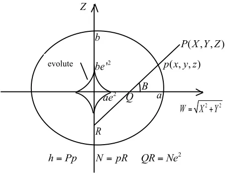
Fig. 1. The relationship between geodetic and Cartesian coordinates, and the ellipsoid evolute.
Step 5: Compute theS-polynomials=S(fi, fj).
Step 6: Compute the remainder following the division of sby theG, denoted bysG.
Step 7: IfsG=0, go to Step 3.
Step 8: AddsGinto setG.G:=G∪ {sG}.
Step 9: UpdateB. B:= B∪ {(g,sG)|g ∈G,g =sG}. Turn to Step 4.
Step 10: Output the reduced Groebner basisG B accord-ing toG.
2.2 Problem formulation based on Lagrange’s con-straint and a Groebner basis
The relationship between Cartesian and geodetic coordi-nates(B,L,h)(B,Lare the latitude and longitude, respec-tively) at any pointP can be constructed according to the following formulae (see Fig. 1):
⎧
major axis, the semi-minor axis, and the eccentricity of the reference ellipsoid, respectively. As we know, the geodetic heighthis the distance from the reference ellipsoid toPin a direction normal to the ellipsoid, so it denotes the shortest distance fromP to the surface of the ellipsoid. Suppose thatpwith Cartesian coordinates(x,y,z)is a point at the surface of the ellipsoid, thus
h2 =min{(X−x)2+(Y−y)2+(Z−z)2}, (2) with a constraint
x2/a2+y2/a2+z2/b2=1. (3) According to Lagrange’s extremum law, we obtain the La-grange equation as
h2 =min{(X−x)2+(Y −y)2+(Z−z)2
+λ(x2/a2+y2/a2+z2/b2−1)}, (4)
whereλis the Lagrange multiplier. By taking the partial derivative of Eq. (4) to x, y, z, and λ, respectively, we
In order to solve the nonlinear polynomial equation, the Buchbergeralgorithm to obtain the Groebner basis of the nonlinear polynomial system of Eq. (5), which has the iden-tical solution to Eq. (5). The obtained Groebner basis in-cludes 16 polynomial elements. If the lexicographic order (x > y > z > λ) is chosen, the corresponding 16 ele-ments are as listed in the Appendix. We note that the first polynomial in the Appendix is a univariate polynomial of degree four inλ, thus we can solve the polynomial equation as follows to obtainλ.
According to Ferrari’s lines (see Shmakov, 2011, and a little revision is made), the four roots of Eq. (6) can be obtained as
Fig. 4. The real number solutions ofpin the region except near the center, the polar axis, and the equatorial plane of the Earth.
(1) Computation ofB
D=(1−e2)x2+y2, (10)
B=arctan(z/D); (11) however, for the case D=0, i.e. B = ±90◦, the Eq. (11) is undefined. It can be computed as follows by the tangent of the half value.
tanB 2 =
sinB 1+cosB =
sinB
cosB+sin2B+cos2B
= z
D+√z2+D2, (12)
thus
B=2 arctan
z/
D+D2+z2
. (13)
Note this formula is fit for the case thatB = ±90◦; namely, the region of the poles.
(2) Computation ofL
By means of Eq. (1), the following expression is ob-tained,
L =arctan(Y/X); (14) however whenX =0, i.e.L = ±90◦, Eq. (14) has no meaning. In the same manner as the computation of B, we can computeLas follows.
tanL 2 =
sinL 1+cosL =
sinL
cosL+sin2L+cos2L
= Y
X+√X2+Y2, (15)
considering its applicability of Eq. (15), we obtain
L=2 arctan Y X+√X2+Y2
exceptY =0, X ≤0. (16) Note it is suitable for any case exceptY =0, X ≤0, i.e.L = ±180◦.
(3) Computation ofh
h =sign(λ)(X−x)2+(Y−y)2+(Z−z)2.
(17) 2.4 Convergence region of the presented algorithm
Table 1. Solution ofpin the region of the polar axis.
Region Real number solutions Complex number solutions Right real number solution
Outside the evolute P1,P2,P3,P4 none P1
On the evolute P1,P2,P3,P4(P2=P4) none P1
Inside the evolute∗ P1,P2 P3,P4 P1
Note:∗denotes that it does not include the region near the center of the Earth.
Table 2. Solution ofpin the region of the equatorial plane.
Region Real number solutions Complex number solutions Right real number solution
Outside the evolute P1,P2,P3,P4 none P1
On the evolute P1,P2,P3,P4(P2=P4) none P1
Inside the evolute∗ P3,P4 P1,P2 P4
Note:∗denotes that it does not include the region near the center of the Earth.
Table 3. Solution ofpin the region except near the center, the polar axis, and the equatorial plane of the Earth. Region Real number solutions Complex number solutions Right real number solution
Outside the evolute P1,P3 P3,P4 P1
On the evolute P1,P2,P3,P4(P2=P4) none P1
Inside the evolute∗ P1,P2,P3,P4 none P1
Note:∗denotes that it does not include the region near the center of the Earth.
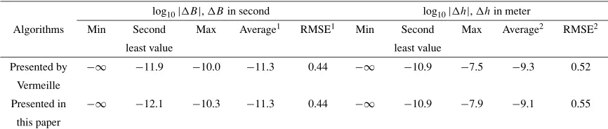
Table 4. Statistics of the errors computed with the algorithms presented by Vermeille and this paper. log10|B|,Bin second log10|h|,hin meter
Algorithms Min Second Max Average1 RMSE1 Min Second Max Average2 RMSE2
least value least value
Presented by −∞ −11.9 −10.0 −11.3 0.44 −∞ −10.9 −7.5 −9.3 0.52
Vermeille
Presented in −∞ −12.1 −10.3 −11.3 0.44 −∞ −10.9 −7.9 −9.1 0.55
this paper
Note: (1) in order to compute the average and RMSE of log10|B|, log10|B|is set to−12.1 if it is less than−12.1; (2) in order to compute the average and RMSE of log10|h|, log10|h|is set to−10.9 if it is less than−10.9.
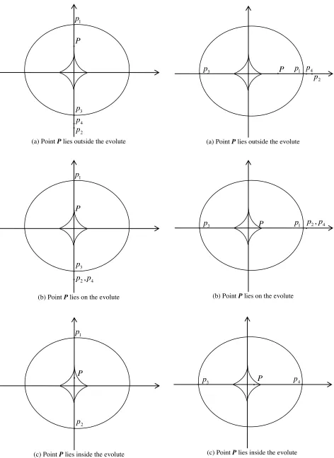
Except for the special regions above, a point in any re-gion, including the equatorial plane, should have its unique geodetic coordinates. However, one can note that the al-gorithm may yield four, at most, solutions of the point p (x,y,z), and this can be explained as follows. The evolute of the reference ellipsoid (see Fig. 1), which is the envelope of all the normal lines through the ellipse surface, is the boundary of judging the number of the solutions of pointp. In the common regions expect the center, the polar axis, and the equatorial plane of the Earth, ifPis outside the evolute (its mathematical equation is(W/ka)2/3+(Z/kb)2/3 =1,
whereka=(a2−b2)/a=ae2,kb=(a2−b2)/b=be2
, andeis the second eccentricity of the reference ellipsoid), it will have two solutions ofp; ifPis on the evolute, it will have three solutions ofp; ifPis inside the evolute, it will have four solutions ofp. This is illustrated in Fig. 4. Only one correct solution ofpis to be selected. And it is neces-sary to turn to numerical analysis for help.
As is known, a polynomial equation in one variable with real coefficients has pairs of conjugate complex number roots, suppose that it has complex number roots. And as a real world matter, the pointp(x,y,z)must have at least one solution. So there are two, or four, real number solutions of
pointp. This agrees with the above geometrical analysis. Next, the correct solution of p will be given for different regions.
(1) Region near the center of the Earth
It is indicated by numerous computations that in the region near the center of the Earth (approximately hav-ing the sphere of radius R = √X2+Y2+Z2 <
0.1 km from the center of the Earth) the solution of the equation is singular. That is to say the algorithm is invalid in this region.
(2) Region of the polar axis of the Earth
The real number solution ofpis shown in Fig. 2, and the solution is summarized in Table 1.
(3) Region of the equatorial plane of the Earth
The real number solution ofpis shown in Fig. 3, and the solution is summarized in Table 2.
(4) Region except near the center, the polar axis, and the equatorial plane of the Earth
The real number solution ofpis shown in Fig. 4, and the solution is summarized in Table 3.
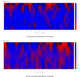
Fig. 5. Contour map of log10|B|,Bin seconds, if the error is less than−12.1, it is set to−12.1.
Table 5. The magnitude of errorhcorresponding to different values ofSalong the polar axis.
S(km) 1 10 20 42.8∗ 100 300 1000 3000 6300
h(m) 103 101 100 10−1 10−2 10−4 10−6 10−8 10−∞
Note:∗denotes that the point lies on the evolute.
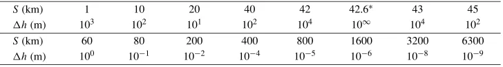
Table 6. The magnitude of errorhcorresponding to different values ofSin the equatorial plane.
S(km) 1 10 20 40 42 42.6∗ 43 45
h(m) 103 102 101 102 104 10∞ 104 102
S(km) 60 80 200 400 800 1600 3200 6300
h(m) 100 10−1 10−2 10−4 10−5 10−6 10−8 10−9
Note:∗denotes that the point lies on the evolute.
Table 7. The magnitude of errorBcorresponding to different values ofSin the region except near the center, the polar axis and the equatorial plane.
S(km) 31 34 78 178 378 1000 3000 6300
B(◦) 10−2 10−4 10−6 10−8 10−10 10−12 10−15 10−15
Table 8. The magnitude of errorhcorresponding to different values ofSin the region except near the center, the polar axis and the equatorial plane.
S(km) 31 34 78 178 378 1000 3000 6300
h(m) 103 102 10−1 10−2 10−4 10−6 10−8 10−9
and 3, can apply for the globe, i.e. B ∈ [−90◦,90◦],L ∈ [−180◦,180◦].
3.
Numerical Experiments and Discussion
3.1 Experiments for the surface, and outer space, re-gions of the Earth
The surface, and outer space, regions of the Earth are the most common regions that geodesy considers. For thou-sands of grid points evenly distributed throughout the entire region withBranging from 0◦to 90◦andhfrom 1 to 108m,
I first compute their Cartesian coordinates, then recover the geodetic coordinates from the Cartesian coordinates apply-ing both the algorithm presented here and that presented by Vermeille (2004). The computation was carried out with the ellipsoid parameter of GRS80. The statistics of errors (B,
h are the errors in latitude and height, respectively) are listed in Table 4. From Table 4, we can see that the algo-rithm presented here is slightly better than that presented by Vermeille forB, but slightly worse forh; however, they are comparable overall and meet the need of any precise geodesy. Figures 5 and 6 depict the distributions ofBand
h, through which the comparison can be made intuitively. 3.2 Experiments for the inner space region of the
Earth
In some special cases, we also need to compute the geodetic coordinates from the Cartesian coordinates for the region below the surface of the reference ellipsoid. The ex-periments adopt the same reference ellipsoid and simulative computation method as described in Subsection 3.1.
(1) Region of the polar axis of the Earth
The simulated computation indicates that the errorB is always zero, and the errorsh are correlated with the distance S between the point Pand the center of the Earth, which is shown in Table 5. It is seen from
Table 5 that the error decreases dramatically with an increase ofS. If an accuracy of one centimeter (com-mon geodetic demand) is required, S must be more than 100 km.
(2) Region of the equatorial plane of the Earth
The simulated computation indicates that the errorB is always zero, and the errors h are correlated to the distance between the pointPand the center of the Earth, which is shown in Table 6. It is seen from Ta-ble 6 that with an increase ofSinside the evolute, the error decreases dramatically to the 10-meter level, and then increases dramatically to+∞; with an increase ofSoutside the evolute, the error again decreases dra-matically. If an accuracy of one centimeter (common geodetic demand) is required, S must be more than 200 km.
(3) Region except near the center, polar axis and equato-rial plane of the Earth
The simulated computation indicates that the errors
B andh are correlated with the distance between the point P and the center of the Earth, which are shown in Tables 7 and 8, taking the case thatB=11◦, L =45◦ for example. It is seen from Tables 7 and 8 that the errorsBandh decrease dramatically with an increase ofS.
Because the algorithm presented by Vermeille (2004) is invalid when the distance between the pointPand the center of the Earth is less than 43 km, I do not compare the two algorithms for this region, and the result is comparable with other regions.
4.
Conclusion
ex-surface, outer, and inner space, of the Earth. The results show that the presented algorithm is comparable to the al-gorithm of Vermeille (2004).
Acknowledgments. The work of this paper is supported by the National Natural Science Foundation of China (Grant No. 41104009), Open Research Fund Program of the Key Laboratory of Geospace Environment and Geodesy, Ministry of Education, China (Grant No. 11-01-04), and the Open Foundation of the Key Laboratory of Precise Engineering and Industry Surveying, Na-tional Administration of Surveying, Mapping and Geoinformation of China (Grant No. PF2011-4). The author is grateful to the sup-port and good working atmosphere provided by his research team in China Three Gorges University. The author also thanks Pro-fessor Kiyoshi Yomogida of Hokkaido University, Japan, Asso-ciate Professor Shinichi Miyazaki of Kyoto University, Japan, and two anonymous reviewers for valuable comments and suggestions, which enhanced the quality of this manuscript.
Appendix.
Borkowski, K. M., Accurate algorithms to transform geocentric to geodetic coordinates,Bull. Geod.,63, 52–54, 1989.
Bowring, B. R., Transformation from spatial to geodetic coordinates,Surv. Rev.,23, 323–327, 1976.
Burnside, W. S. and A. W. Panton,Theory of Equations, Dublin Univ. Press Series, p. 121–125, 1904.
Featherstone, W. E. and S. J. Claessens, Closed-form transformation be-tween geodetic and ellipsoidal coordinates,Stud. Geophys. Geod.,52, 1–18, 2008.
Feltens, J., Vector method to compute the Cartesian (X,Y,Z) to geodetic (φ, λ,h) transformation on a triaxial ellipsoid,J. Geod.,83, 129–137, 2009.
Fukushima, T., Fast transform from geocentric to geodetic coordinates,J. Geod.,73, 603–610, 1999.
Fukushima, T., Transformation from Cartesian to geodetic coordinates accelerated by Halley’s method,J. Geod.,79, 689–693, 2006. Gonzalez-Vega, L. and I. Polo-Blanco, A symbolic analysis of Vermeille
and Borkowski polynomials for transforming 3D Cartesian to geodetic coordinates,J. Geod.,83, 1071–1081, 2009.
Jones, G. C., New solutions for the geodetic coordinate transformation,J. Geod.,76, 437–446, 2002.
Paul, M. K., A note on computation of geodetic coordinates from geocen-tric (Cartesian) coordinates,Bull. Geod.,108(2), 135–139, 1973. Pollard, J., Iterative vector methods for computing geodetic latitude and
height from rectangular coordinates,J. Geod.,76, 36–40, 2002. Shmakov, S. L., A universal method of solving quartic equations,Int. J.
Pure Appl. Math.,71, 251–259, 2011.
Vermeille, H., Direct transformation from geocentric coordinates to geode-tic coordinates,J. Geod.,76, 451–454, 2002.
Vermeille, H., Computing geodetic coordinates from geocentric coordi-nates,J. Geod.,78, 94–95, 2004.
Zhang, C. D., H. T. Hsu, X. P. Wu, S. S. Li, Q. B. Wang, H. Z. Chai, and L. Du, An alternative algorithm to transform Cartesian to geodetic coordinates,J. Geod.,79, 413–420, 2005.