Numerical simulation and FRAP experiments show that the plasma membrane binding protein PH-EFA6 does not exhibit anomalous sub-diffusion in cells.

Numerical simulation and FRAP experiments show

that the plasma membrane binding protein PH-EFA6

does not exhibit anomalous sub-diffusion in cells.

Cyril Favard1,∗ ID

1 _{Membrane Domains and Viral Assembly, IRIM, UMR 9004 CNRS - Université Montpellier, 1919, route de} Mende, 34 000 Montpellier, France; [email protected]

* Correspondence: [email protected]

Abstract:FRAP technique have been used for decades to measure movements of molecules in 2D. Data obtained by FRAP experiments in cell plasma membranes are assumed to be described through means of two parameters, a diffusion coefficient D (as defined in a pure Brownian model) and a mobile fraction M. Nevertheless, it has also been shown that recoveries can be nicely fit using anomalous sub-diffusion. FRAP at variable radii has been developed using the Brownian diffusion model to access geometrical characteristics of the surrounding landscape of the molecule. Here we performed numerical simulations of continuous time random walk (CTRW) anomalous subdiffusion and interpreted them in the context of variable radii FRAP. These simulations were compared to experimental data obtained at variable radii on living cells using the PH domain of the membrane binding protein EFA6 (exchange factor for ARF6, a small G protein). This protein domain is an excellent candidate to explore the structure of the interface between cytosol and plasma membrane in cells. By direct comparison of our numerical simulations to the experiments, we show that this protein does not exhibit anomalous diffusion in BHK cells. The non Brownian PH-EFA6 dynamics observed here is more related to spatial heterogeneities such as cytoskeleton fences effects.

Keywords:Anomalous diffusion; FRAP; Numerical Simulations; PH - Domain, Membrane Binding

1. Introduction

16

Early models of the plasma membrane, notably the fluid mosaic model [1] postulated that

17

transmembrane proteins were freely diffusing in a sea of lipids. During these two last decades, it

18

has become apparent that cell surface membranes are far from being homogeneous mixture of their

19

lipid and protein components. They are compartmented into domains whose composition, physical

20

properties and function are different. Numerous studies on transmembrane proteins and plasma

21

membrane lipids by means of single particle tracking (SPT), Fluorescence Correlation Spectroscopy

22

(FCS) or fluorescence recovery after photobleaching (FRAP) has shown the existence of micrometer and

23

nanometer size domains on both model membrane [2,3] and living cells[4–6]. In the plasma membrane

24

of living cells, these domains can come from different origins, but are generally classified into two

25

main groups :

26

• "rafts" model where lipid/lipid phase separation drives the lateral partitioning of transmembrane

27

proteins. [7]

28

• "cytoskeleton fence" model in which transmembrane proteins are coralled by a fence of

29

cytoskeleton just beneath the plasma membrane. [8,9]

30

Variable radii FRAP first [5,6], then spot variation FCS [10–12] helped in discriminate amongst

31

these two models the nature of the deviation to pure Brownian diffusion of membrane components in

32

living cells.

33

FRAP experiments have been used for determination of long-range molecular diffusion of proteins

34

and lipids on both model system and cells for more than 30 years [13,14]. Briefly, fluorescently labelled

35

molecules localized within a predefined area are irreversibly photo-destructed by a short and intense

36

laser pulse. The recovery of the fluorescence in this area is then measured against time. Since

37

no reversible photoreaction occurs, recovery of the fluorescence in the photobleached area is due

38

to diffusion. FRAP data are generally interpreted by assuming classical Brownian diffusion. Two

39

parameters can then be obtained : D, the lateral diffusion coefficient and M, the mobile fraction of the

40

diffusing molecule. When the radius of the photobleached area is small compared to the diffusion area,

41

M must be equal to 1 for freely diffusing species. In fact, most of the data reported so far in biological

42

membranes for transmembrane proteins shows a value of M < 1. This lack in total fluorescence

43

recovery can be interpreted as a restriction to free-diffusion behaviour. Parameters obtained have then

44

to be re-evaluated to recognize the effect of time-dependent interactions in a field of random energy

45

barriers.

46

An experimental approach to that question has been proposed by Federet al.[15] by introducing

47

anomalous (sub)diffusion in the motion of transmembrane proteins. Many sources of motion restriction

48

can lead to anomalous diffusion (for review see [16] and [17]. Saxton has performed extensive

49

numerical simulations to help in identifying the sources of anomalous diffusion (obstacles, binding...)

50

using SPT measurements [18,19] and he declined this more recently to FRAP experiments [20] using

51

fractional Brownian motion (fBm) or continuous time random walk (CTRW) models as sources of

52

anomalous diffusion.

53

Membrane bound proteins should also be submitted to several interactions with their surrounding

54

environment that should account for an anomalous subdiffusion behaviour. Sources of deviation from

55

Brownian motion in their lateral diffusion may include lipid domains trapping, binding to immobile

56

proteins and/or obstruction by cytoskeletal elements. This different possible interactions can exhibit

57

different characteristic times, or different distributions of characteristic times. Here, diffusion of an

58

intracellular membrane-bound protein domain (pleckstrin homology domain of EFA6, the ARF6

59

exchange factor) has been analysed inside living cells by FRAP experiments. Previous studies have

60

shown that these proteins are linked to the polar head ofPI(4, 5)P2lipids by means of electrostatic

61

interactions[21]. Furthermore, the protein used in this study appears to have a functional requirement

62

to be associated to the plasma membrane within cells [22,23]

63

In this paper, numerical simulation of the CTRW model of anomalous sub-diffusion were first

64

performed at a single spot size. Based on the quality of the fit using different analytical expression,

65

we tested the ability to retrieve this anomalous diffusion in the simulated recovery curves first and in

66

the experimental one afterwards. We showed that performing FRAP experiments at a single spot size

67

did not allow to discriminate between the CTRW induced anomalous diffusion case and the empirical

68

classical approach using mobile and immobile fraction.

69

We then computed and performed experimental FRAP at variable radii. By plotting changes in

70

the anomality of the diffusion or in the mobile fraction as a function of the inverse of the bleached

71

radius, as in Saloméet al.[5] we showed that it was possible to discriminate between the two models.

72

Interestingly we observed that the restriction to the mobility of the PH-EFA6 domain is not due to

73

CTRW anomalous sub diffusion, but more certainly to the sub cortical actin fences.

2.1. Anomalous sub-diffusion Modeling

A way to describe the continuous time random walk sub-diffusion is to start from a two dimensional random diffusion process. A particle walks from trap to trap and spend a certain (random) time in each trap. It is characterized by the following operation :

r→r+∆;t→t+τ (1)

randtare respectively the two dimensional position and the age of the particle, where∆is a two

77

dimensional random (Gaussian) variable with variancev=2D, andτis the (random) time the particle

78

spend into the trap.

79

In our model, the particle is supposed to diffuse very rapidly between two traps. This travel time

80

is therefore neglected (this, because it was not experimentally accessible). The timeτthe particle stays

81

in a trap is supposed to have very strong fluctuations, this give rise to anomalous diffusion pattern.

82

As an example a generic distribution is used which leads, after a while, to a standard Levy law in time :

P0(τ) = α

(1+τ)α+1 (2)

This distribution have been used in the same type of context by Naggle [24].

83

The Levy exponentαis the characteristic exponent of subdiffusive behaviour. For long times we

have :

<r2(t)>∝tα ₍₃₎

Whenα<1 a spatio-temporal Fourier (Laplace) analysis leads to the following asymptotic (ω,k

84

→0) Green function :

85

˜

g(k,ω) = 1

ω(Dαk2ω−α+1)

;Dα=D/Γ(1−α) (4)

whereωandkare respectively the conjugate variables of positionrand timet, wherek=|k|.

86

Notice that the solution of the inverse Laplace transform is a function of the variablek2tα_{. It follows}

87

that the Green function is a function of the variablex=r2/tα_{. Whenxis high enough one can perform}

88

an approximate inverse transformation via a saddle point method :

89

g(r,t) ∝ exp(−cst xν_{) ; ν=} 1

2−α, cst: a known constant (5)

Notice that the exponent ν interpolate nicely between the gaussian case (α = 1) and the

exponential case. The general solution of this type of anomalous diffusion process is then :

ρ(r,t) = Z

ρ0(r0−r)g(x(r0,t))d2r0 (6)

whereρis the probability density to find the particle at the pointrat instanttandρ0is the initial

90

state.

91

As the Green function is a bell-shaped fast decreasing function, one approximate it by a Gaussian

92

shape with the exact dispersion,Dα = Dsin(πα)/(πα), which can be calculated from eq.4. This

93

permits to construct an analytical expression of the fluorescence recovery using standard properties of

94

Gaussian functions.

95

Starting from Axelrod [13] initial density as it is immediately after a Gaussian laser beam profile extinction indeed :

ρ0(r) =exp(−Kexp(−2

r2

(K=photobleaching constant, depending on experimental conditions [13]) and using the standard

96

properties of the Gaussian shape in the convolution operation, one can obtain the time evolved result

97

as a series.

98

Once integrated upon a disk of radiusR, and, after normalization to the surface of the disk, one

99

obtain the FRAP signal :

100

IR(t) = 1+

∞

∑

1

(−K)n n!

1 2n

1−exp

− 2nR

2

R2_+4nD

αtα

(8)

This function will be used to fit experimental data.

101 102

Systematic corrections of this procedure are determined using numerical Monte-Carlo simulations

103

of the fluorescence recoveries, using knownαandD=Dα

(πα)

sin(πα)

104

In order to keep in our calculation the finite size effects, the simulation were made in a ring of a

105

radius of 30 arbitrary unit (a.u.) length explored by 107particles for each recovery. Radii varying from

106

0.5 to 3 a.u. were photo-destructed during the simulation. Reflective type of boundary conditions

107

were used. This means that when a particle gets out of the 30 a.u. radius it is re-introduced in the

108

same direction at a small distance of the boundary. See AppendixAfor examples of recovery curves

109

generated numerically by this approach.

110

2.2. Validating numerical simulation and analytical models

111

In order to verify the validity of our analytical model, a set of numerically simulated recovery

112

curves using anomalous diffusion as a model has been fitted with equation8. Each parameter (αand

113

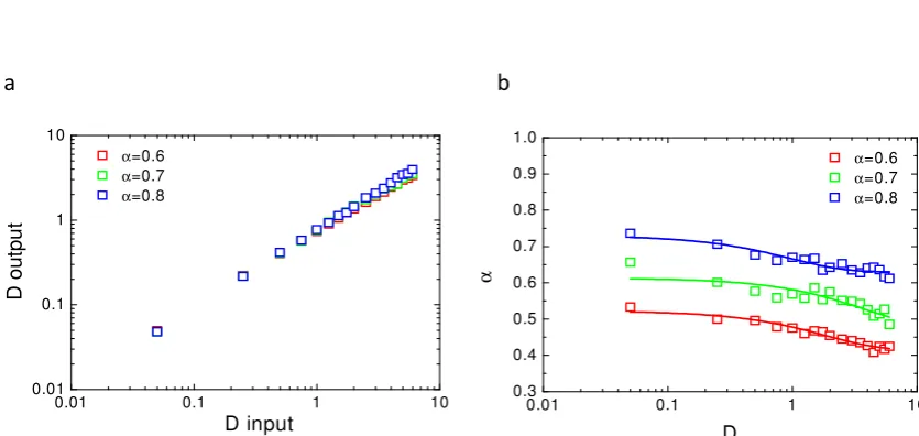
D) were tested. Figure1a shows the value ofDobtained after fit of the numerical (Doutput) simulation

114

using givenD(Dinput) for the three differentαtested above. Figure1b illustrates the variation of fitted

115

αas a function ofDused in the simulation, forα=0.6 (red);α=0.7 (green);α=0.8 (blue). This clearly

116

shows that both parameters (α,D) are always underestimated when fitting with an analytical model

117

the numerically simulated fluorescence recoveries.

0.01 0.1 1 10 0.01

0.1 1 10

α=0.6 α=0.7 α=0.8

D

o

u

tp

u

t

D input

a

b

0.01 0.1 1 10

0.3 0.4 0.5 0.6 0.7 0.8 0.9 1.0

α=0.6 α=0.7 α=0.8

α

D

Figure 1. Values of the parameters (D,α) obtained from the fit of the simulated recoveriesa- D values obtained after fit of the fluorescence recovery with eq.8(Doutput) as a function of D values used

in the numerical simulation (Dinput) for differentα. Note that the slope is always less than 1 b- Values

ofαobtained after fit of the simulated curves with eq.8for differentαused in the simulation and as a function of the D values used in the simulation. Note that the originalαvalue used in the simulation is never reached by fit of the simulated recoveries.

This is mainly due to the finite size and finite time effect of our numerical simulations and

119

paradoxically is also nicely mimicking what could occur experimentally in a finite size cell reservoir.

120

2.3. Challenging analytical models to identify numerically simulated anomalous diffusion fluorescence recoveries

121

Fluorescence recoveries have been numerically simulated using CTRW anomalous diffusion as

122

the model of molecular motion. These curves were then fitted with three different analytical expression

123

of FRAP recoveries, each being specific of a diffusion model :

124

• Anomalous diffusion motion (aDm): see eq.8in section2.1

125

• Free Brownian motion (Bm) :

126

IR(t) =

∞

∑

1

(−K)n n!

1 1+n+8nDt

R2

(9)

• Restricted Brownian motion (rBm) :

IR(t) = (1−M)1

−e−K

K +M

∞

∑

1

(−K)n n!

1

1+n+8nDt_R2 (10)

where M accounts for the mobile fraction.

0.1 1 10 100 0.8 0.9 1 L o g (N o rm. F lu o . R e co v e ry)

Log t (s)

1 10 100 0.3 0.4 0.5 L o g (N o rm . F lu o . R e co ve ry)

Log t (s)

0 20 40 60 80 100

0.8 0.9 1.0 N o rma lize d F lu o re sce n ce R e co ve ry t(s)

0 20 40 60 80 100

0.3 0.4 0.5 N o rma lize d F lu o re sce n ce R e c o ve ry t(s)

a

b

c

d

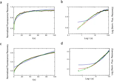
Figure 2. Best fits using the different models of Normal and Log-Log plots of simulated CTRW anomalous sub-diffusion recoveries.α=0.6 is the value used for the simulation in the four plots. In blue, Bm model (eq.9), in red rBM model (eq.10) and in green aDm (eq.8) fits. Ina & bD=2 and inc & dD=0.1.a & care the normal plots whileb & dare the log-log plots. From these graph it can be seen that one can hardly distinguish between the rBm model (red) and the aDm model (green) fits of the simulated recovery.

Figure2shows the obtained results for the three tested models (aDm in green, fBm in blue, rBm

128

in red) with two different values ofDαand withα=0.6. It can easily be seen that the fBm does not

129

fit to the curve, as expected, but surprisingly it can also be seen that aDm and RBm models fit quasi

130

equivalently the numerical simulation. Even log-log plot (Fig. 2b and d) hardly allows to directly

131

separate the two-models. Still log-log plots show that these models can be discriminated at short times

132

(t«τc,τcbeing the characteristic half-time of the recovery) and at very long times( t»τc).

133

2.4. Single spot FRAP does not allow to identify the nature of PH-EFA6 diffusion in cells.

134

FRAP experiments have been performed on 15 different BHK cells (3 recoveries per cells on

135

average) expressing the PH domain of EFA6 linked to the GFP. These data have been acquired at a

136

given radius using the 63x objective (see experimental section for explanation). EFA 6, an exchange

137

factor for ARF 6 (a small G protein) has recently been described as being located on the internal part of

138

the plasma membrane, with its PH domain responsible for the interaction with lipids [23].

0.1 1 10

0.5 1

L

o

g

(

N

o

rm

.

F

lu

o

.

R

e

c

o

v

e

ry

)

Log t(s)

0 20 40 60 80

0.0 0.2 0.4 0.6 0.8 1.0

N

o

rm

a

liz

e

d

F

lu

o

re

s

c

e

n

c

e

R

e

c

o

v

e

ry

t(s)

a

b

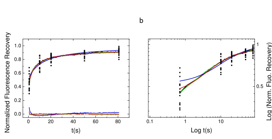
Figure 3. Average experimental recovery curve fitted by the three diffusion models. The three models (bM, rBm and aDm) were used to fit the average recovery curve obtained from 45 different experiments. The normal (parta) plot shows the residual from the fit of the different models. Note that only the bM model fit is inaccurate. The Log-Log plot (partb) illustrate again the difficulty to discriminate between the aDm and the rBm model in the goodness of the fit.

Figure3shows the average fluorescence recovery (black line, mean of the 45 recoveries) as well as

140

some points extracted from of the 45 different recoveries in order to illustrate the discrepancy observed

141

when working with cells. This mean fluorescence recovery has been fitted by the three different models

142

used in the previous section. On the bottom of Fig.3a is depicted the differences between the fit and the

143

observed fluorescence (Ff−Fo) in order to illustrate the quality of the fit. From figure3a (normal plot)

144

and figure3b (log-log plot) it can easily be seen that except for the free Brownian motion model(Bm),

145

the nature of the diffusion of PH-EFA6 cannot be discriminated between restricted Brownian motion

146

(rBm) and anomalous diffusion (aDm). This is confirmed by aχ2statistical test to probe the quality

147

of the fit as shown in table1. Table1also summarized the average values of the set of parameters

148

(D,M,Dα,α) that can be extracted from the different fits.

149

Table 1.Parameters values obtained by the fit of the average experimental recovery with the different analytical models

Model D(µm.s−1) M α Dα(µm.s−α) χ2

Bm 0.12±0.06 1 - - 5.7±0.5

rBm 0.22±0.01 0.92±0.01 - - 3.8±1.6

aDm - - 0.65±0.02 1.48±0.05 2.9±1.6

2.5. Variable radii FRAP allows correct estimation of the anomalous sub-diffusion exponentα

150

Previous results using direct analysis on both numerically simulated recoveries and experimental

151

recoveries clearly showed that : i) ParametersαandDα) of the aDm model were always underestimated

152

ii) aDm and rBm models could only be discriminated at short and long times. Nevertheless, since time

153

and space are correlated in diffusion and since experimental time-scale is finite, variable radii FRAP

154

experiments were firstly numerically simulated and performed after on cells (see experimental section

for explanation). Each parameter (αandDα) were estimated again, by fitting simulated recoveries at

156

different radius (see Monte-Carlo simulation section for explanation) with our analytical model (eq.8).

157

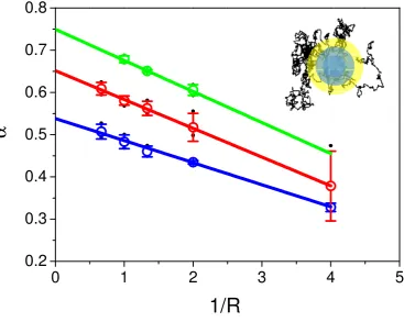
Figure4shows the behaviour of fitted a as a function of 1/R. Theory of anomalous diffusion processes

158

predicts that a is space-invariant in a “homogeneously heterogeneous” environment. It can be directly

159

seen on the plot that this is not what our data suggest, but on the opposite they showed that a linear

160

dependence ofαas a function of 1/R (at least for R > 1 a.u.) with a negative slope is observed for the

161

three tested values of a (α=0.6 in blue,α=0.7 in green,α=0.8 in red). Intercept of this linear regression

162

(R→∞) leads to values closed to the inputαin the numerical simulation.

163

0

1

2

3

4

5

0.2

0.3

0.4

0.5

0.6

0.7

0.8

α

1/R

Figure 4. Values ofαobtained from the fit of CTRW simulated recoveries as a function of1/R. Values ofαintroduced in the fit were respectively 0.6 (in blue), 0.7 (in red), 0.8 (in green). Dots represent the mean±s.d. values ofαobtained with the fit using eq. 8of simulated recoveries for a set of D values (0.01, 0.05, 0.1, 0.5, 1, 2, 3, black dots in the graph). Extrapolation at 1/R=0 of the linear fit of the differental phaobtained from the fits of recoveries at different radius givesal phavalues close to the one used for the simulations.

Similar results were obtained when plottingDfitted as a function of 1/R . Therefore, in order to

164

test the hypothesis thatαandDcould be correctly determined by performing linear regressions of

165

fitted values of both parameters as a function of 1/R, a set of numerical simulation were performed

166

using differentD,αand R. Values ofαandDat 1/R=0 intercepts are resumed in Appendix fig.A2.

167

Fig.A2a andA2b show that, except for few values, when using this approach,αandDcan be estimated

168

with an error of less than 5 % of their real values. With regards to the discrepancy of the experiments

169

on cells, this uncertainty seems enough accurate for correct determination of both parameters in case

170

of anomalous diffusion processes using variable radii.

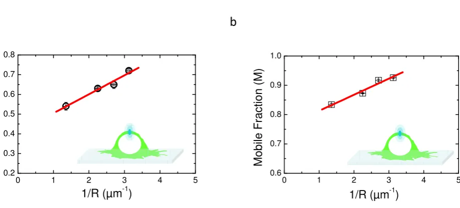
domains in cells [5]. They found both by numerical simulation and by experimental approaches that

174

fitting recovery curves using the rBm model lead to a linear regression of the mobile fraction (M) as a

175

function of 1/R with a positive slope. In this study our results show that the same approach is valid

176

with aDm model and that plotting of a as a function of 1/R led to a linear regression with a negative

177

slope. Therefore several experiments (n<30) has been performed on cells expressing the PH domain

178

of EFA6 at variable radii of photodestruction. Experimental recoveries were fitted with both models

179

(aDm and fBm).

180

0 1 2 3 4 5

0.2 0.3 0.4 0.5 0.6 0.7 0.8

α

1/R (µm

)

0 1 2 3 4 5

0.6 0.7 0.8 0.9 1.0

M

ob

ile

F

rac

ti

o

n

(M

)

1/R (µm

)

a

b

Figure 5. Comparison of the two models aDm and rBm using vrFRAP in the case of PH-EFA6 diffusion at the plasma membrane of BHK cells a: Plot of α values obtained by fitting the experimental recoveries with eq.8as a function of 1/R. The plot exhibit a positive slot in opposite to the one observed in Fig.4, suggesting an absence of a CTRW anomalous sub-diffusion in the motion of PH-EFA6.b: Plot of M value obtained by fitting the experimental recoveries with eq.10as a function of 1/R. The plot exhibit a positive slope as obsreved in [25] and [5], suggesting a diffusion with trapping in spatial domains.

Figure5shows the behaviour of the characteristic parameters of each model (αfor aDM and M for

181

rBm) as a function of 1/R. In Fig.5a is depicted the linear dependence of experimentalαas a function

182

of 1/R. This results clearly show a positive slope for the regression, suggesting that the aDm model is

183

not the correct model for the analysis of diffusion in the case of PH-EFA6 in this experimental time and

184

length scale. On the opposite, Fig.5b, where M is plotted as a function of 1/R clearly shows a positive

185

slope as already observed in Salomé’s work [5]. This shows that, in the case of PH-EFA6 diffusion at

186

the plasma membrane of BHK cells, the rBm is the more appropriate model to describe the restriction

187

of diffusion observed in FRAP experiments.

Schramet al.empiricaly determined a relationship between the size of the trapping domains (L) and the variation of the mobile fraction (M) [25] :

M=Mp+0.63.L

R ;L<R (11)

Using eq.11, we could determine that 75% of PH-EFA6 molecules exhibit free diffusion while the

189

25 % left are confined in domains of approximately 90 nm radius.

190

3. Discussion

191

This work has been initiated to characterize the nature of the diffusion of molecules binding

192

the inner leaflet of the cell plasma membranes by means of FRAP experiments. In a first attempt,

193

we decided to compare experimental data obtained with the PH domain of EFA6 expressed in BHK

194

cells to FRAP curves generated from anomalous sub-diffusive particles numerically simulated. Then,

195

we analyzed the recoveries with three different diffusion models, namely the pure Brownian motion

196

(Bm), the restricted Brownian motion (rBm) and the CTRW anomalous subdiffusion (aDm). Four

197

parameters can be extracted from these diffusion models. The Brownian diffusion coefficientDand

198

the mobile fraction M (M=1 in the case of Bm) on one side, and the anomalous subdiffusion exponent

199

αand its related anomalous diffusion coefficent Dα on the other side. The aDm model has been

200

extensively studied by numerical simulations. Direct analysis of numerically simulated curves lead to

201

an underestimation ofDαandα. This was already observed by Federet al.whom proposed, in order to

202

circumvent this underestimation, to add a mobile fraction (M) as a new parameter [15]. On a physical

203

point of view this is incorrect since the phenomenological parameter “mobile fraction” is indeed a part

204

ofαas discussed by Nagleet al.[24]. This underestimation ofDαandαis mainly due to finite size effect

205

(space and time) that cannot be easily overcome neither in simulations nor in experiments. We directly

206

tested for anomalous sub-diffusion in the simulated and experimental curves by fitting the recovery

207

curves with normal and anomalous equations and look for systematic deviations of the fit, both in

208

linear plots to see the fit at large times and log-log plots to see the fit at short times. From this approach

209

we could see that the Bm can be immediately discarded. The difference between the aDm and the fBm

210

could only be observed at very short times (log-log plots) and very long times. Unfortunately, these

211

two extrema times are hardly easy to analyse in experiments. Indeed, at short times the curve may be

212

distorted by diffusion during the bleach pulse [26] and limits in the frequency of data collection. At

213

long times, motion of the membrane or photobleaching of the fluorescent probe might appear. This is

214

illustrated here in our experimental data. Fits of single spot fluorescence recoveries did not allow to

215

determine without uncertainties which of the aDm or the rBm model reflect the nature of PH-EFA6

216

diffusion at the plasma membrane of BHK cells. Although underestimated, theαvalue we found here,

217

when fitting with the aDm model, reflect a strong deviation from the Brownian motion and suggest

218

that PH-EFA6 explores a strongly compartmentalized landscape while travelling at the inner leaflet of

219

the plasma membrane. Nevertheless, thisαvalue, as well as the M value in the case of the rBm model

220

are higher than the one found for IgE receptor transmembrane protein in RBL cells (α=0.46±0.22)

221

[15]. Using single particle tracking experiments, other transmembrane proteins such as MHC class I in

222

HeLa cells has also been shown to exhibit anomalous subdiffusion with anαvalue close to 0.5 [27]. On

223

the opposite, other transmembrane proteins exhibit highαvalues (α=0.8) (Kv2.1 potassium channel

224

in HEK293T cells [28]) or pure Brownian motion (MHC class II in CHO cells [29] or aquaporin-1 in

225

MDCK cells [30].

226

The inability of FRAP to cover several time decades as SPT or FCS techniques can be overcome

227

by probing the environment at different space scale using variable radii FRAP [5,6]. Here we have

228

simulated recoveries in the case of CTRW anomalous subdiffusion at different space scales and fit them

229

with the aDm model in order to extract the set of parameters (α,D). By monitoring the change of fitted

230

(α,D) parameters as a function of space (1/R) we observed that the fitted values ofαdecreased with

231

decreasing radius of observation. We showed that the correct values ofαandDcould be determined

anomalous subdiffusion is not the correct model to describe the motion of PH-EFA6 in BHK cells. On

236

the opposite, when monitoring the change of the mobile fraction obtained by fitting the experimental

237

recoveries with the rBm model, we observed the same tendency as the one described in [5] and [31], i.e.,

238

an increase of the mobile fraction with a decreasing radius. Using this approach, we could determine

239

that 25% of PH-EFA6 molecules are confined in domains of 90 nm radius.

240

CTRW is not the only source of anomalous sub-diffusion. The experimental increase ofαwith

241

decreasing radius can also be an apparent consequence of a cross over regime with two different

242

diffusion coefficient as it is described by the rBm model in this study. Using FCS experiments and

243

simulations at different radii of a two phases two component lipid mixtures at different temperature,

244

Favardet al. showed that changes in anomalous sub-diffusion exponentαcould nicely predict the

245

phase transitions temperatures but failed in determining the average size of domains coexisting in

246

the two-phases [2]. On the opposite by monitoring the change in diffusion regimes, they could nicely

247

determine the mean size of the gel-phase domains. If we extend this approach to oural phaplot as

248

a function of the probes radius, we see that the transition from anomalous sub-diffusion (α<1) to

249

normal diffusion (α=1) occurs at radius of 160 nm, i.e., not far from the values obtained with the rBm

250

model.

251

The range of domain sizes observed here (90 to 160 nm radius), independently of the model used

252

to describe the dynamics of PH-EFA6, is likely to be due to subcortical actin cytoskeleton. Equivalent

253

sizes has been observed in NRK cells [32] using electron microscopy, and recently in several cell lines,

254

by monitoring membrane lipids dynamics using STED-FCS [33]. Interestingly, Krapfet al.described

255

that this meshwork has a fractal dimension and could therefore lead to anomalous sub-diffusion [34].

256

Therefore, further investigations and numerical simulations using a meshwork with fractal dimension

257

as the origin of the anomalous sub-diffusion are likely to be conducted in order to understand the

258

origin of ourα= f(1/R)behaviour in our vrFRAP experiments.

259

In conclusion, by performing FRAP at variable radii, we found a way to discriminate CTRW

260

induces anomalous sub-diffusion from other restricted motion at the plasma membrane of living

261

cells. We also show that, while travelling at the inner leaflet of the plasma membrane, PH-EFA6 is not

262

stopped in various traps with different residence times but on the opposite is mainly freely diffusing

263

with on average 25% of the molecules confined in 90-160 nm radius open domains most probably due

264

to the actin cortical cytoskeleton.

265

4. Materials and Methods

266

4.1. Monte Carlo Simulation

267

In order to keep in our calculation the finite size effects, the simulation were made in a ring of

268

a radius of 30 arbitrary unit (a.u.) length explored by 106 particles for each run. Radii varying from

269

0.5 to 3 a.u. were photo-destructed. Reflective type of boundary conditions were used. This means

270

that when a particle gets out of the 30 a.u. radius it is re-introduced in the same direction at a small

271

distance of the boundary.

272

4.2. Cell culture and transfection

273

Baby hamster kidney cells (BHK) were grown on a coverslip in BHK-21 medium (Gibco-BRL),

274

containing 5% FCS, 10% Tryptose phosphate broth, 100U/ml penicillin, 100µg/ml stretomycin and

275

2mM L-Glutamine. Cells were transfected using Fugene 36 hours before the FRAP experiments with a

276

pC1EGFPPHEFA6 plasmid. Fugene containing medium was replaced 12 h before the experiments by

277

fresh medium. pC1EGFPPHEFA6 contains the sequence for both PH-EFA6 domain and EGFP as a

fluorescent label, linked to the N-terminus of the PH-EFA6 domain in order to avoid any perturbation

279

to the membrane linkage.

280

4.3. FRAP experiments

281

FRAP measurements were made with a commercially available confocal microscope, Leica

282

TCS-SP1 (Leica Microsystems, Germany). Prebleached images were firstly acquired to ensure for the

283

lack of photo-destruction during the observation. A brief laser pulse (200 ms) was then delivered to the

284

cell on a given and fixed position. Images were thereafter recorded at given intervals (440 ms) using a

285

spectral window for fluorescence emission between 500 and 600 nm. The intensity ratio between the

286

extinction laser beam and the monitoring laser beam was fixed to 106. Each fluorescence recovery was

287

recorded for 100 s at 25◦C, containing 150 experimental values (Recovery curve was sampled every

288

0.44 s in the beginning and 1 s in the end to avoid photobleaching during the monitoring). Focusing

289

the laser by the microscope objectives produced a Gaussian intensity distribution of the beam in the

290

object plane. This distribution was monitored using NBD-PC labelled DPPC multilamellar preparation

291

at 25◦C (T<Tm). Since no diffusion occurs at this temperature, the image obtained immediately after

292

the end of the bleaching pulse shows a "hole" in the fluorescent preparation that allow measurement of

293

the laser waist and determination of the intensity profile in the x,y plane. These measurements were

294

confirmed by the use of fluorescent beads with a maximum wavelength of emission at 500 nm [35].

295

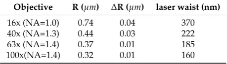
The following values were obtained for the waist as a function of the objective used :

296

Table 2.Size of the different radius measured with the objectives used in this work.

Objective R (µm) ∆R (µm) laser waist (nm)

16x (NA=1.0) 0.74 0.04 370

40x (NA=1.3) 0.44 0.03 222

63x (NA=1.4) 0.37 0.01 185

100x(NA=1.4) 0.32 0.01 160

Funding:‘This research received no external funding”

297

Acknowledgments: Author would like to acknowledge M. Franco for the gift of the PH-EFA6 plamsid and

298

discussion. I am indebted to JL Meunier for the numerical simulations of the FRAP recoveries. The author

299

also thank A. Lopez and N. Olivi-Tran for fruitful discussions. THe author is a member of the IMABIO CNRS

300

consortium. Most of this work has been realized during the author stay at the IPMC CNRS UMR 7275.

301

Conflicts of Interest:“The authors declare no conflict of interest.”

302

Abbreviations

303

The following abbreviations are used in this manuscript:

304 305

FRAP Fluorescence Recovery After Photobleaching

vrFRAP variable radii Fluorescence Recovery After Photobleaching FCS Fluorescence Coreelation Spectroscopy

SPT Single Particle Tracking

CTRW Continuous-Time Random Walk aDm anomalous subdiffusion motion

Bm Brownian motion

rBm restricted Brownian motion

PH-EFA6 Pleckstrin Homology domain of Exchange Factor for ARF-6

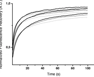
Figure A1. Monte-Carlo simulation of normalized fluorescence recoveries in the case of CTRW anomalous subdiffusion . Different values ofDandαhave been tested in the simulations. Here, values ofD=0.5; 1; 1.5 are represented from bottom to top with differentαin each case : 0.6 (dots) ; 0.7 (thin line) ; 0.8 (thick line). The Monte Carlo has been constructed with 107_{individual trajectories}

Appendix A. Examples of Numerical Generated Fluorescence Recovery Curves

307

FigureA1depicts some fluorescence recovery curves obtained with our numerical simulations

308

for different D andαinserted in the simulation.

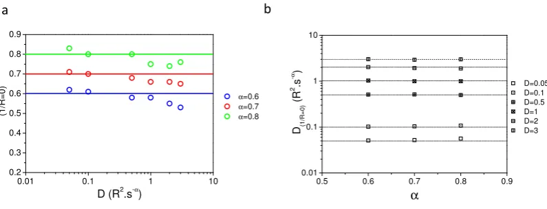
0.5 0.6 0.7 0.8 0.9 0.01

0.1 1 10

D=0.05 D=0.1 D=0.5 D=1 D=2 D=3

D(1

/R

=

0

)

(

R

2 .s

-α )

α

0.01 0.1 1 10

0.2 0.3 0.4 0.5 0.6 0.7 0.8 0.9

α=0.6

α=0.7

α=0.8

α (1

/R

=

0

)

D (R2.s-α)

a b

Figure A2. Values ofα(fig.A2a) andD(fig.A2b) at1/R=0intercepts.

Appendix B. Comparison of input and fitted D andαat variable radii

310

In figureA2are plotted values ofα(fig.A2a) andD(fig.A2b) at 1/R=0 intercepts. Fig.A2a

311

andA2b show that extrapolatedα_(1/R=0)and extrapolatedD_(1/R=0)are found to be with an error of

312

less than 5 % of their simulation inserted values.

175, 720–731. doi:10.1126/science.175.4023.720.

316

2. Favard, C.; Wenger, J.; Lenne, P.F.; Rigneault, H. FCS diffusion laws in two-phase lipid membranes:

317

determination of domain mean size by experiments and Monte Carlo simulations. Biophysical journal2011,

318

100, 1242–1251. doi:10.1016/j.bpj.2010.12.3738.

319

3. Hac, A.E.; Seeger, H.M.; Fidorra, M.; Heimburg, T. Diffusion in two-component lipid membranes–a

320

fluorescence correlation spectroscopy and monte carlo simulation study. Biophys. J.2005,88, 317–333.

321

doi:10.1529/biophysj.104.040444.

322

4. Edidin, M.; Kuo, S.C.; Sheetz, M.P. Lateral movements of membrane glycoproteins restricted by dynamic

323

cytoplasmic barriers. Science1991,254, 1379–1382. doi:10.1126/science.1835798.

324

5. Salomé, L.; Cazeils, J.L.; Lopez, A.; Tocanne, J.F. Characterization of membrane domains by frap

325

experiments at variable observation areas. Eur Biophys J1998,27, 391–402. doi:10.1007/s002490050146.

326

6. Yechiel, E.; Edidin, M. Micrometer-scale domains in fibroblast plasma membranes. The Journal of Cell

327

Biology1987,105, 755–760. doi:10.1083/jcb.105.2.755.

328

7. Lingwood, D.; Simons, K. Lipid rafts as a membrane-organizing principle. Science2010,327, 46–50.

329

doi:10.1126/science.1174621.

330

8. Kusumi, A.; Sako, Y.; Yamamoto, M. Confined lateral diffusion of membrane receptors as studied by single

331

particle tracking (nanovid microscopy). Effects of calcium-induced differentiation in cultured epithelial

332

cells. Biophysical Journal1993,65, 2021–2040. doi:10.1016/S0006-3495(93)81253-0.

333

9. Sako, Y.; Kusumi, A. Compartmentalized structure of the plasma membrane for receptor movements as

334

revealed by a nanometer-level motion analysis. J. Cell Biol.1994,125, 1251–1264.

335

10. Wawrezinieck, L.; Rigneault, H.; Marguet, D.; Lenne, P.F. Fluorescence correlation spectroscopy

336

diffusion laws to probe the submicron cell membrane organization. Biophys. J.2005,89, 4029–4042.

337

doi:10.1529/biophysj.105.067959.

338

11. Lenne, P.F.; Wawrezinieck, L.; Conchonaud, F.; Wurtz, O.; Boned, A.; Guo, X.J.; Rigneault, H.; He,

339

H.T.; Marguet, D. Dynamic molecular confinement in the plasma membrane by microdomains and the

340

cytoskeleton meshwork.EMBO J.2006,25, 3245–3256. doi:10.1038/sj.emboj.7601214.

341

12. Eggeling, C.; Ringemann, C.; Medda, R.; Schwarzmann, G.; Sandhoff, K.; Polyakova, S.; Belov, V.N.; Hein,

342

B.; von Middendorff, C.; Schönle, A.; Hell, S.W. Direct observation of the nanoscale dynamics of membrane

343

lipids in a living cell. Nature2009,457, 1159–1162. doi:10.1038/nature07596.

344

13. Axelrod, D.; Koppel, D.E.; Schlessinger, J.; Elson, E.; Webb, W.W. Mobility measurement by

345

analysis of fluorescence photobleaching recovery kinetics. Biophysical Journal1976, 16, 1055–1069.

346

doi:10.1016/S0006-3495(76)85755-4.

347

14. Soumpasis, D.M. Theoretical analysis of fluorescence photobleaching recovery experiments. Biophysical

348

Journal1983,41, 95–97. doi:10.1016/S0006-3495(83)84410-5.

349

15. Feder, T.J.; Brust-Mascher, I.; Slattery, J.P.; Baird, B.; Webb, W.W. Constrained diffusion or

350

immobile fraction on cell surfaces: a new interpretation. Biophysical Journal 1996, 70, 2767–2773.

351

doi:10.1016/S0006-3495(96)79846-6.

352

16. Bouchaud, J.P.; Georges, A. Anomalous diffusion in disordered media: Statistical mechanisms, models and

353

physical applications.Physics Reports1990,195, 127–293. doi:10.1016/0370-1573(90)90099-N.

354

17. Hoefling, F.; Franosch, T. Anomalous transport in the crowded world of biological cells. Rep. Prog. Phys.

355

2013,76, 046602. WOS:000317032800007, doi:10.1088/0034-4885/76/4/046602.

356

18. Saxton, M.J. Anomalous diffusion due to obstacles: a Monte Carlo study. Biophysical Journal1994,

357

66, 394–401. doi:10.1016/S0006-3495(94)80789-1.

358

19. Saxton, M.J. Anomalous diffusion due to binding: a Monte Carlo study. Biophysical Journal1996,

359

70, 1250–1262. doi:10.1016/S0006-3495(96)79682-0.

360

20. Saxton, M.J. Anomalous Subdiffusion in Fluorescence Photobleaching Recovery: A Monte Carlo Study.

361

Biophysical Journal2001,81, 2226–2240. doi:10.1016/S0006-3495(01)75870-5.

362

21. Hyvönen, M.; Macias, M.J.; Nilges, M.; Oschkinat, H.; Saraste, M.; Wilmanns, M. Structure

363

of the binding site for inositol phosphates in a PH domain. The EMBO Journal, 14, 4676–4685.

364

doi:10.1002/j.1460-2075.1995.tb00149.x.

22. Franco, M.; Peters, P.J.; Boretto, J.; Donselaar, E.v.; Neri, A.; D’Souza-Schorey, C.; Chavrier, P. EFA6, a sec7

366

domain-containing exchange factor for ARF6, coordinates membrane recycling and actin cytoskeleton

367

organization.The EMBO Journal1999,18, 1480–1491. doi:10.1093/emboj/18.6.1480.

368

23. Macia, E.; Partisani, M.; Favard, C.; Mortier, E.; Zimmermann, P.; Carlier, M.F.; Gounon, P.; Luton, F.;

369

Franco, M. The pleckstrin homology domain of the Arf6-specific exchange factor EFA6 localizes to the

370

plasma membrane by interacting with phosphatidylinositol 4,5-bisphosphate and F-actin.The Journal of

371

biological chemistry2008,283, 19836–19844. doi:10.1074/jbc.M800781200.

372

24. Nagle, J.F. Long tail kinetics in biophysics? Biophysical Journal 1992, 63, 366–370.

373

doi:10.1016/S0006-3495(92)81602-8.

374

25. Schram, V.; Tocanne, J.F.; Lopez, A. Influence of obstacles on lipid lateral diffusion: computer simulation of

375

FRAP experiments and application to proteoliposomes and biomembranes.Eur Biophys J1994,23, 337–348.

376

doi:10.1007/BF00188657.

377

26. Waharte, F.; Brown, C.M.; Coscoy, S.; Coudrier, E.; Amblard, F. A two-photon FRAP analysis of

378

the cytoskeleton dynamics in the microvilli of intestinal cells. Biophys. J. 2005, 88, 1467–1478.

379

doi:10.1529/biophysj.104.049619.

380

27. Smith, P.R.; Morrison, I.E.; Wilson, K.M.; Fernández, N.; Cherry, R.J. Anomalous diffusion of major

381

histocompatibility complex class I molecules on HeLa cells determined by single particle tracking. Biophys.

382

J.1999,76, 3331–3344. doi:10.1016/S0006-3495(99)77486-2.

383

28. Weigel, A.V.; Simon, B.; Tamkun, M.M.; Krapf, D. Ergodic and nonergodic processes coexist in the plasma

384

membrane as observed by single-molecule tracking. Proc. Natl. Acad. Sci. U.S.A.2011,108, 6438–6443.

385

doi:10.1073/pnas.1016325108.

386

29. Vrljic, M.; Nishimura, S.Y.; Brasselet, S.; Moerner, W.E.; McConnell, H.M. Translational diffusion

387

of individual class II MHC membrane proteins in cells. Biophys. J. 2002, 83, 2681–2692.

388

doi:10.1016/S0006-3495(02)75277-6.

389

30. Crane, J.M.; Verkman, A.S. Long-range nonanomalous diffusion of quantum dot-labeled aquaporin-1 water

390

channels in the cell plasma membrane. Biophys. J.2008,94, 702–713. doi:10.1529/biophysj.107.115121.

391

31. Baker, A.M.; Saulière, A.; Gaibelet, G.; Lagane, B.; Mazères, S.; Fourage, M.; Bachelerie, F.; Salomé, L.; Lopez,

392

A.; Dumas, F. CD4 interacts constitutively with multiple CCR5 at the plasma membrane of living cells. A

393

fluorescence recovery after photobleaching at variable radii approach. J. Biol. Chem.2007,282, 35163–35168.

394

doi:10.1074/jbc.M705617200.

395

32. Morone, N.; Fujiwara, T.; Murase, K.; Kasai, R.S.; Ike, H.; Yuasa, S.; Usukura, J.; Kusumi, A.

396

Three-dimensional reconstruction of the membrane skeleton at the plasma membrane interface by electron

397

tomography.J. Cell Biol.2006,174, 851–862. doi:10.1083/jcb.200606007.

398

33. Andrade, D.M.; Clausen, M.P.; Keller, J.; Mueller, V.; Wu, C.; Bear, J.E.; Hell, S.W.; Lagerholm, B.C.; Eggeling,

399

C. Cortical actin networks induce spatio-temporal confinement of phospholipids in the plasma membrane

400

– a minimally invasive investigation by STED-FCS.Scientific Reports2015,5, 11454. doi:10.1038/srep11454.

401

34. Sadegh, S.; Higgins, J.L.; Mannion, P.C.; Tamkun, M.M.; Krapf, D. Plasma Membrane is Compartmentalized

402

by a Self-Similar Cortical Actin Meshwork. Phys. Rev. X2017,7, 011031. doi:10.1103/PhysRevX.7.011031.

403

35. Schneider, M.B.; Webb, W.W. Measurement of submicron laser beam radii. Appl Opt1981,20, 1382–1388.