Article
1
Hydrodynamic and Hydrographic Modeling of
2
Istanbul Strait
3
Mehmet Melih Koşucu 1*, Mehmet Cüneyd Demirel 1, V.S. Ozgur Kirca1 and Mehmet Özger 1
4
1 Istanbul Technical University, Civil Engineering Faculty, Hydraulics Division; [email protected],
5
[email protected], [email protected], [email protected]
6
* Correspondence: [email protected];
7
8
Abstract: The aim of this study is to model hydrodynamic processes of the Istanbul Strait with its
9
stratified flow characteristic and calibrate the most important parameters using local and global
10
search algorithms. For that two open boundary conditions are defined, which are in the North and
11
South part of the Strait. Observed bathymetric, hydrographic, meteorological and water level data
12
are used to set up the Delft3D-FLOW model. First, the sensitivities of model parameters on the
13
numerical model outputs are assessed using PEST toolbox. Then, the model is calibrated based on
14
the objective functions focusing on the flowrates of upper and lower layers. The salinity and
15
temperature profiles of the Strait are only used for model validation. The results show that the
16
calibrated model outputs of Istanbul Strait are reliable and consistent with the in-situ measurements.
17
The sensitivity analysis reveals that the Spatial Low-Pass Filter Coefficient, Horizontal Eddy
18
Viscosity, Prandtl-Schmidt Number, Slope in log-log Spectrum and Manning Roughness Coefficient
19
are most sensitive parameters affecting flowrate performance of the model. The agreement between
20
observed salinity profiles and simulated model outputs is promising whereas the match between
21
observed and simulated temperature profiles is weak showing that the model can be improved
22
particularly for simulating the mixing layer.
23
Keywords: Istanbul Strait; stratified flow; gravity driven flow; numerical modelling
24
25
1. Introduction
26
Istanbul Strait is one of the most prominent straits in the World. Due to the constructional,
27
navigational and deep see discharge activities, understanding the flowrates of the Istanbul Strait
28
bears importance. The Strait connects Black Sea (in the North) and the Marmara Sea (in the South)
29
providing continuous water exchange between these two water bodies. For centuries, the
30
hydrodynamical and hydrographical structure of the Strait has been the subject of many research
31
efforts and broad discussions dating back to centuries ago.
32
Ç eçen et al. [1] made observations, and established a mathematical model of the Istanbul Strait.
33
Salinity and temperature profiles of Istanbul Strait are visualized in 4 different seasons of 1980.
34
Bayazıt and Sümer [2], in a continuation of Ç eçen et al.’s study, reported the salinity and water mass
35
balance equations. Results of these studies agreed with observations. Sumer and Bakioğlu [3],
36
proposed a one-dimensional mathematical model utilizing the observations from Anadolu Kavağı
37
(North) and Ü sküdar (South) stations. Sumer and Bakioğlu [3] stated that water level variations
38
between two sides of the Strait have a strong impact on the stratified flow structure. Latif et al. [4]
39
asserted that the density-driven lower layer flow in the Strait could not reach the Black Sea from time
40
to time, especially when the strong Northerly winds blow. These winds, generating a significant shear
41
force on the Strait, could blockade the lower layer flow such that it could not continue towards Black
42
Sea direction. In addition, when the river discharges into the Black Sea increases, freshwater entrance
43
to the Strait rises. Water level rising in the Black Sea can also blockade lower layer flow [5]. Falina et
44
al. [6] ascertained that “Mediterranean Originated Water” intruded to Black Sea’s 100-600 m depths
45
through Istanbul Strait during strong cyclonic storms.
46
Sur et al. [7] indicated that the Danube River's impact on Black Sea water level was much
47
stronger than the other rivers flowing into the Black Sea. When the Danube River’s flowrate rises, an
48
increment on the discharge of upper layer flux of the Strait occurs. Oğuz et al. [8] established a
49
mathematical model, and stated that there were three control zones termed as "Hydraulic Controls"
50
of the Strait. Two of these are located in the Northern and Southern parts of the Strait (two silled
51
zones), whereas the third is the narrowest section of the Strait. These zones are significant for the
52
hydrodynamics of the Strait since “Maximal Exchange" events occur in these locations [9], [10], [11].
53
This events are characterized with the enhanced mixing between the lower and upper layers of the
54
Strait. Dorrell et al. [12] mentioned the “internal hydraulic jump” in the Istanbul Strait, which occurs
55
in the Hydraulic Control sections. As very well known, during the normal hydraulic jump, Froude
56
Number becomes near to unity while the flow regime switches from subcritical to supercritical.
57
However, it could be said that there is no critical value of stratified depth-averaged Froude Number,
58
on the contrary of Normal Hydraulic Jump. Beşiktepe et al. [13] made observations, and conducted
59
measurements with ADCP and CTD devices in the Turkish Straits. Based on these activities, salinity,
60
temperature, and current velocity profiles were developed. Ö zsoy et al. [14] executed current velocity
61
and flowrate measurements in the Turkish Straits, and consequently described the structure of
62
Istanbul Strait as outstanding because of its maximal exchange issue. Gregg et al. [15] stated that the
63
flow condition of the Strait is at "Quasi-Steady State". Gregg and Ö zsoy [16] expressed opinions about
64
this "Quasi-Steady State" flow conditions. According to these considerations, when upper layer flow
65
enters the Marmara Sea, and lower layer flow enters the Black Sea, flow regimes are supercritical.
66
Moreover, bottom friction is required to evaluate the hydrodynamic structure of the Strait. Güler et
67
al. [17] made long-period velocity measurements at various points in the Istanbul Strait. The
68
measurements were conducted between May and September of 2003, which represent the
69
hydrodynamic condition of the summer season. Yüksel et al. [18] built up velocity profile of the Strait,
70
and asserted that current regime of the Strait was evaluated from wind and atmospheric pressure, as
71
well as fresh water from rivers discharging into the Black Sea. Aydoğan et al. [19] modeled the current
72
velocities of the Strait with Artificial Neural Networks (ANN) method. In the mentioned study, the
73
advantages and disadvantages of the ANN method were evaluated accurately about the prediction
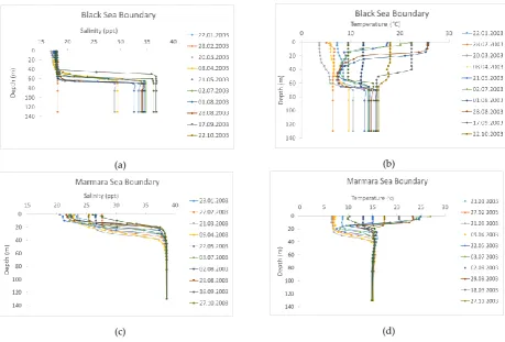
74
of Istanbul Strait’s current velocity. Jarosz et al. [20] commented on ADCP and CTD data in the Strait
75
between September 2008 and February 2009. Altiok and Kayışoğlu [21] executed current velocity,
76
temperature and salinity measurements with ADCP and CTD devices during 11 and 15 years,
77
respectively. Even if some certain mean values were given for upper and lower layer fluxes, the flux
78
values differed from North to South [22]. Because of maximal exchange phenomena in the Hydraulic
79
Control sections, upward entrainment fluxes from the lower layer to upper layer increase the upper
80
layer flowrate. Therefore, upper layer flowrate values are generally larger in the North section of the
81
Strait compared to the South.
82
Akay [23] proposed a numerical modeling study of the Istanbul Strait conducted with
83
Telemac3D software. In that study, an unstructured grid and finite element method were used. Akay
84
took the Southern boundary conditions as discharge values which are osculated to study of Ö zsoy et
85
al. [14], and Northern boundary conditions as free-water level and current velocity values. Ö ztürk
86
[24] established a numerical model of the Strait with an unstructured grid, which was based on the
87
finite volume method with MIKE 3 software. Water level, salinity and temperature values were
88
estimated as boundary conditions. After the running of the model, it was observed that measured
89
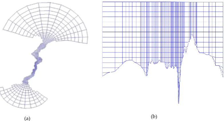
and modeled current velocity values were in accordance. Sözer [25], and Sözer and Ö zsoy [26]
90
numerically modeled Istanbul Strait by use of the ROMS (Regional Ocean Modeling System) software,
91
which was based on the finite volume method. For Black Sea boundary conditions, Şile water level
92
measurements were used, and for Marmara Sea boundary conditions Yalova water level
93
measurements were input. Salinity and temperature boundary conditions were entered as constant
94
with depth and stratification was maintained. It was concluded that stratified boundary transport
95
model of the whole Turkish Straits. In this study, Özsoy et al.’s [14] measurements, Sözer's [25]
97
Istanbul Strait model results, and the whole Turkish Straits System's (TSS) model results were
98
compared. According to Sannino et al’s [27] study, the whole TSS model represents an accordance
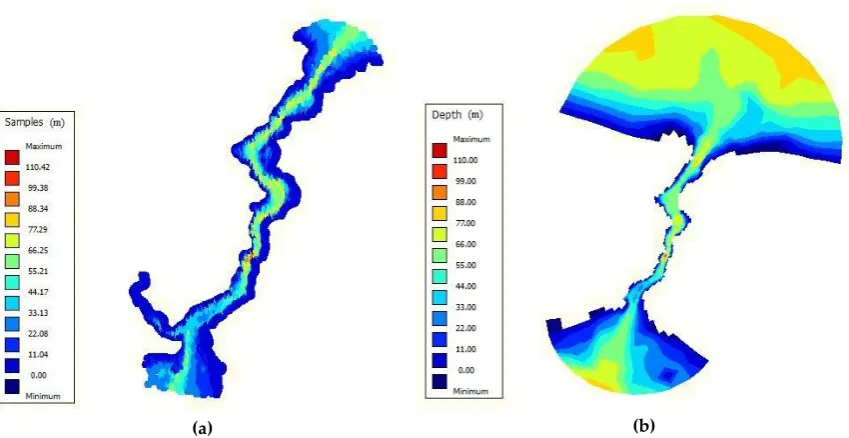
99
with the in-situ observations. Strait of Gibraltar presents another two-layered dynamic system which
100
is similar to Istanbul Strait [28]. Except the tidal dynamics, modeling the Strait of Gibraltar bears
101
affinity with modeling Istanbul Strait [29]. Although there have been many studies conducted to
102
solve the hydrodynamics and/or hydrography of this sophisticated two-layer system, none of the
103
previous studies focused on the sensitivity of the results against the input parameters used in the
104
model. Furthermore, unlike many of the previous studies, the present study facilitates a direct
105
comparison of numerical modeling results with the in-situ hydrographic data, namely salinity and
106
temperature profiles along the Istanbul Strait.
107
In the present study, a numerical hydrodynamic model of Istanbul Strait is established using the
108
DELFT3D-FLOW, which is a open source hydrodynamic simulation software utilizing finite
109
differences method and a structured grid system [30]. The objective of the study is two folds; (1) to
110
assess the sensitivity of the flow regime against different input parameters in order to select most
111
important parameters for the calibration and (2) to calibrate the model using local and global
112
algorithms to simulate both the hydrodynamics and hydrography of the two-layer flow system. To
113
represent the real conditions occurring in the Strait, the proposed model was calibrated against
114
flowrates of the upper and lower layers, and tested using the salinity and temperature measurements.
115
With the numerical results, the hydrodynamics of the stratified flow in the Istanbul Strait is evaluated.
116
2. Materials and Methods
117
The uniqueness of physical and hydrodynamic characteristics of Istanbul Strait has attracted the
118
interest of researchers for decades. The physical structure of the Istanbul Strait presents a natural
119
channel shape, which is meandering, widening, narrowing, deepening, and shoaling. Net length of
120
Istanbul Strait is 31 km. The maximum depth is 110 m, minimum depth is nearly 30 m, and the widest
121
and narrowest sections are 3500 m and 700 m in width, respectively (Figure 1).
122
123
124
As mentioned above, the most significant feature of the flow in Istanbul Strait is that there are
126
two different flows in the upper and lower layers in opposite directions. In Figure 2, the longitudinal
127
section of the strait is given with a schematic representation of the flow structure. While the upper
128
layer flow is towards North from the Black Sea to the Marmara Sea, the lower layer flow is towards
129
South from the Marmara Sea to the Black Sea. Less salty (hence lighter) Black Sea water constitutes
130
the upper layer of the Strait. Upper Layer is colder than the lower layer in winter months and warmer
131
in the summer months. The lower layer is saltier than the upper layer, and coming from the
132
Mediterranean Sea [4]. The intermediate (mixing) layer lies between the upper and lower layers and
133
the thickness of this layer oscillates with the effect of internal waves.
134
Figure 2. Schematic description of the longitudinal section of the Istanbul Strait based on [2]-.
135
For setting up a reliable numerical model, bathymetric, mareographic, hydrographic and
136
meteorological data are essential. For the present study, bathymetric data was obtained from Turkish
137
Navy Office of Navigation, Hydrography and Oceanography.
138
Water level differences between two sides of the Strait -which governs the hydrodynamic
139
structure of the flow through the Strait- are used as input forcing in the model. For this purpose,
140
mareographic data of the 2003 year was obtained from the Turkish Naval Forces. Southern and
141
Northern boundaries of the Strait are represented by water level data of Pendik and Anadolu Kavağı
142
stations, respectively, as shown in Figure 3.
143
144
Figure 3. Daily water level values in Pendik and Anadolu Kavağı mareography stations in 2003.
145
As stated above, the main reason for the stratification of the Strait is the density variation by
146
depth. Two main factors affecting density variation, salinity and temperature, are incorporated in the
147
hydrodynamic model. Salinity and temperature variation data were taken from the ISKI (Istanbul
148
are selected for the Northern boundary, whereas the station M23 is chosen for the Southern boundary,
150
which are shown in Figure 1. For two boundaries of the Strait, monthly observations of salinity and
151
temperature data are used as input parameter in the model (Figure 4).
152
Figure 4. First row shows a) salinity in Black Sea b) temperature in Black Sea and second row shows c)
153
salinity in Marmara Sea d) temperature in Marmara Sea boundaries of the Istanbul Strait.
154
For modeling the hydrodynamical structure of the Istanbul Strait, meteorological data is
155
required to include the effect of atmosphere-sea interaction taking place at the near-surface part of
156
the water mass, since wind shear and barometric differences are important flow forcing factors, as
157
well as the water level and density differences. To serve as input data for the model, mean sea level
158
pressure values, and wind velocity components u (direction in east-west) and v (direction in
north-159
south) at 10 m altitude are obtained from ECMWF database.
160
2.1. Model Setup
161
The hydrodynamic model of the Istanbul Strait is established in Delft3D-FLOW. This model is
162
based on finite element method and often used in hydrodynamical modeling of Coasts, Rivers,
163
Estuaries, and Seas with governing equations of fluid dynamics [32]. These equations are the
Navier-164
Stokes equations which also includes Reynolds stresses (RANS equations) with the k- closure. It
165
should be noted that Delft3D-FLOW operates with hydrostatic pressure instead of solving the whole
166
suit of RANS equations. Details can be found in [32].
167
To set up the hydrodynamic model in Delft3D-FLOW following steps are applied: (1)
168
computational grid generation, (2) input of bathymetric conditions, (3) input of other parameter
169
values, (4) initial conditions assignment, (5) boundary conditions assignment, and (6) selection of
170
observation point the locations (locations for model output).
171
To simulate fluid motions, continuity and momentum equations (RANS equations) should be
172
solved. However, these equations –especially momentum equations- are in the form of non-linear
173
partial differential equations. Since these equations are non-linear, it is not possible to solve them
174
analytically. Numerical finite difference method is used to approach the exact solution of these
175
(a) (b)
equations in a computationally-efficient manner. The computational grid, which is an important part
176
of the solution scheme, was generated by discretizing the flow domain using the RGFGRID module
177
of Delft3D. In the model, horizontal and vertical grids were used. The horizontal grid facilitates the
178
representation of the fluid motions throughout the Strait in the North-South direction (Figure 5a).
179
Horizontal Grid domain used in the model covers the region between 30.0354 and 28.0944 longitudes
180
and 41.4756 and 40.7878 latitudes. Total horizontal grid cell quantity is 685. Maximum and minimum
181
grid lengths are 6161 m and 198 m, respectively. Coarse (≈ 6000 m) section of the computational grid,
182
corresponds to open sea zones. The grid spacing gets finer inside of Istanbul Strait for maintaining
183
the computational efficiency as well as computational accuracy.
184
Vertical grid is also important to observe the stratification effect. Unlike many of previous
185
research [33] [34] [35], z-model was used in this study in favor of -model, meaning that the number
186
of grid cells in the vertical were not constant but variable as a function of depth. This is because,
z-187
model is known to be more capable to accurately model stratified flow conditions [32]. As shown in
188
Figure 5b, the vertical grid lines are perpendicular. Nevertheless, perpendicularity of grids is
189
distorted occasionally, especially in near-bottom regions. But in the Intermediate Layer,
190
perpendicularity is intact and avails stratification of the flow field. All vertical grid lengths are taken
191
as constant at 5 m.
192
(a) (b)
Figure 5. Hydrodynamic Grid of the Model (a) vertical and (b) horizontal directions
193
Bottom topography of the Strait exhibits an irregular and variable shape. Figure 6 shows the
194
point-based (raw data) and refined area based bathymetry. Refined bathymetry is established in
195
QUICKIN module of Delft3D by triangular interpolation method. This way a more realistic
196
(a) (b)
Figure 6. Point-based (raw) (a) and area-based (refined) bathymetry data of the Strait (b)
198
There are several other input parameters in the model such as time-related parameters,
199
roughness, viscosity and turbulence parameters. Time-related parameters include the time domain
200
and time step parameters. Time domain of the numerical run starts at 01.01.2003 – 00:00:00 and
201
finishes at 01.01.2004 – 00:00:00. Time step is chosen as 0.25 minutes (15 seconds) i.e. small enough to
202
accurately capture the unsteady behavior of the flow. Five of the input parameters: (1) Manning
203
Roughness Coefficient, (2) Horizontal Eddy Viscosity, (3) Slope in Log-Log Spectrum, (4)
Prandtl-204
Schmidt Number, and (5) Spatial Low-Pass Filter are designated as calibration parameters. Vertical
205
eddy viscosity and diffusivity parameters are 10-4 m2/s and 10-5 m2/s [32]. As mentioned above, k-𝜺
206
Turbulence Model is selected in the model.
207
Water level values at both ends of the Strait were chosen for the hydrodynamic open-boundary
208
conditions. Like mentioned above, as the Northern boundary conditions, Anadolu Kavağı water level
209
data (Figure 3), and as the Southern boundary conditions, Pendik water level data (also in Figure 3)
210
are dictated to the model as input.
211
As the transport boundary conditions, hydrographic (salinity and temperature) data is used. For
212
Northern boundary conditions, the data given in Figure 4a and 4b are used, whereas the data
213
presented in Figure 4c and 4d are adopted for Southern boundary conditions.
214
The initial conditions value of four model parameters were needed to be defined, which were
215
water level, velocity, salinity, and temperature. In the model, the initial water level and velocity
216
values are assumed as 0, termed as "Cold Start". This means that the boundary conditions will
217
determine the flow structure of the model substantially. As salinity and temperature, average values
218
of Figure 4 are adopted. For instance, average values of Figure 4a and 4c, give us a representative
219
salinity data for the whole domain. In the same way, the mean values of Figure 4b and 4d, conceive
220
initial temperature values.
221
In order to calibrate the model by flowrates, two different techniques are used in addition to the
222
manual calibration: 1) gradient based Levenberg Marquardt [36] [37] [38] 2) Covariance Matrix
223
Adaptation Evolution Strategy (CMA-ES) [39] [40]. Levenberg-Marquardt (LM) method finds the
224
local best solution, whereas CMA-ES is a global metaheuristic search algorithm.
225
3. Results
226
Before the calibration process, the most sensitive parameters that affect the model results are
227
determined using one-at-a-time local sensitivity analysis method based on Jacobian matrix in PEST
228
toolbox [36]. Initially, number of calibration parameter candidates were 17. These parameters are
229
Eddy Diffusivities; Wind Stress Coefficients A, B and C; Wind Speed Coefficients A, B and C; Secchi
231
Depth; Stanton and Dalton Numbers; Slope in log-log Turbulence spectrum; Prandtl-Schmidt
232
Number; and Spatial low-pass filter coefficient. Relative sensitivity values of these parameters,
233
evaluated by Levenberg-Marquardt Method, are given in Table 1. According to this sensitivity
234
analysis, Spatial Low-Pass Filter Coefficient, Horizontal Eddy Viscosity, Prandtl-Schmidt Number,
235
Slope in log-log Spectrum, and Manning Roughness Coefficient are the parameters on which the
236
model results have the highest sensitivity. Therefore, these 5 parameters are selected for the model
237
calibration using LM and CMA-ES methods.
238
Table 1. Sensitivity analysis results using PEST tool [37] [38]
239
Parameter Normalized Sensitivity
Index Sensitivity Level
Manning Roughness Coefficient 0.1696 Medium
Horizontal Eddy Viscosity 0.5352 High
Horizontal Eddy Diffusivity 0.0122 Low
Vertical Eddy Viscosity 0.0195 Low
Vertical Eddy Diffusivity 0.0975 Low
Wind Stress Coefficient A 0.0073 Low
Wind Speed Coefficient A 0.0052 Low
Wind Stress Coefficient B 0.0975 Low
Wind Speed Coefficient B 0.0975 Low
Wind Stress Coefficient C 0.0975 Low
Wind Speed Coefficient C 0 Low
Secchi Depth 0 Low
Stanton Number 0 Low
Dalton Number 0 Low
Slope in log-log Spectrum 0.2869 Medium
Prandtl-Schmidt Number 0.5188 High
Spatial Low-Pass Filter Coefficient 1.0000 Highest
After the sensitivity analysis, important parameters are selected and calibrated as shown in
240
Table 2.
241
Table 2 shows that, PEST-LM yielded the most realistic value as far as the Manning roughness
242
coefficient is concerned. For the Istanbul Strait, having a non-vegetated naturally formed seabed, a
243
textbook guess for the Manning roughness coefficient would be around 0.025-0.035 [41]. While 0.02
244
is quite below this expected range, the value calibrated by PEST-LM method successfully captures
245
this range.
246
Table 2.Calibrated values of the model parameters using three methods
247
Parameter Manual PEST-LM CMA-ES
Manning Roughness Coefficient 0.02 0.0304 0.023
Horizontal Eddy Viscosity (m2/s) 1 9.8598 10
Slope in log-log Spectrum -5/3 -1.6390 -1.6667
Prandtl-Schmidt Number 0.7 0.8087 0.7
Spatial Low-Pass Filter Coefficient 0.3 0.2950 0.3333
Likewise for the horizontal eddy viscosity, a value around at the order of 10 m2/s is much more
248
realistic than value around 1 m2/s, considering the mesh (grid) size adopted in the present study is at
249
the order of hundreds to thousands of meters, and the enhanced resistance due to sub-grid turbulence
250
should be accounted for in the horizontal eddy viscosity value.
251
When it comes to the other calibration parameters given in Table 2, the values achieved by all
252
literature. To sum up, among the three methods employed, PEST-LM proved to yield the most
254
physically consistent values for all the parameters.
255
Flowrates calculated by the model were extracted as model output in the sections which are
256
located in the Northernmost and the Southernmost parts of the Strait. To test the reliability of the
257
flowrate results of the model, ensemble-averaged monthly mean flowrate measurements for each
258
month from 1999 to 2010 were taken into consideration as shown in Table 3 [21]. In this table, lower
259
layer flowrate values directed to North are shown as negative while velocity vectors of Southward
260
flow in the upper layer are assumed as positive.
261
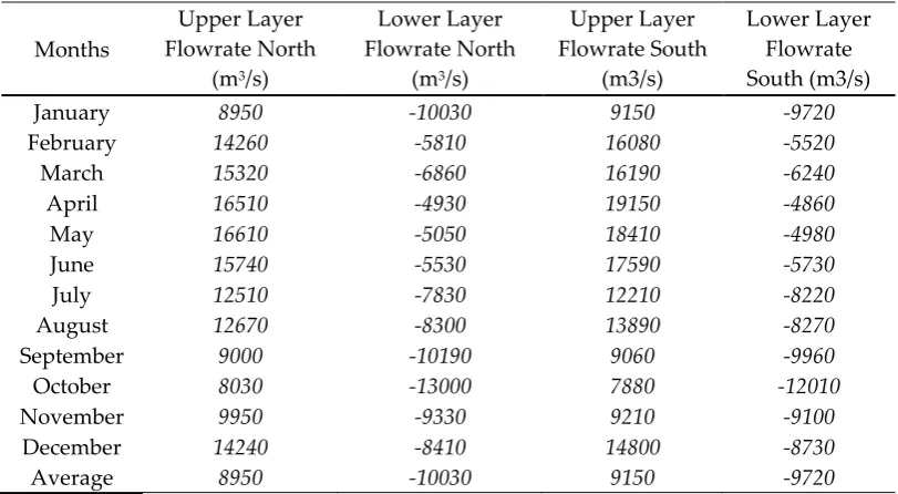
Table 3. The average of 10 years in-situ flowrate values which are measured in North and South of
262
the Strait [21].
263
Months
Upper Layer Flowrate North
(m3/s)
Lower Layer Flowrate North
(m3/s)
Upper Layer Flowrate South
(m3/s)
Lower Layer Flowrate South (m3/s)
January 8950 -10030 9150 -9720
February 14260 -5810 16080 -5520
March 15320 -6860 16190 -6240
April 16510 -4930 19150 -4860
May 16610 -5050 18410 -4980
June 15740 -5530 17590 -5730
July 12510 -7830 12210 -8220
August 12670 -8300 13890 -8270
September 9000 -10190 9060 -9960
October 8030 -13000 7880 -12010
November 9950 -9330 9210 -9100
December 14240 -8410 14800 -8730
Average 8950 -10030 9150 -9720
3.1. Hydrodynamic Model Calibration
264
In this study, the monthly average flowrate values (from January to December) computed by the
265
numerical model are compared with the ensemble-averaged monthly mean values of the 10 years
in-266
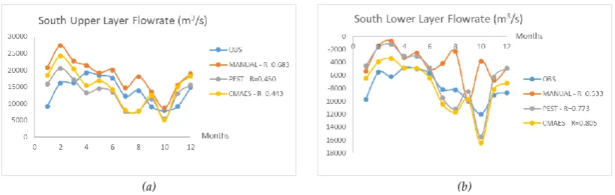
situ observations. Figure 7 and 8 show the modeled and observed monthly average flowrate for the
267
lower and upper layers at the Northern and Southern part of the Strait.
268
When Figure 7 and 8 are investigated, it can apparently be seen that the Levenberg-Marquardt
269
calibration algorithm (PEST-LM) is the best fitting method generally [36] . Especially in the Northern
270
part of the Strait, agreement of PEST-calibrated model output with the observed values is remarkable.
271
On the other hand, PEST-LM method cannot said to be the most efficient method for calibration.
272
When it comes to the South station measurements, manual calibration and CMA-ES performed
273
slightly better than the PEST-LM method.
274
(a) (b)
(a) (b)
Figure 8. Upper (a) and Lower (b) Flowrate values of Southern Part of the Strait
276
According to Figure 7 and 8, it is understood that, observations and modeled flowrates are in
277
accordance generally. One can easily see that North and South flowrates are not the same. This
278
difference between flowrates originates from the mixing taking place between the lower and upper
279
flow layers. For instance, a water element travelling from the Marmara Sea through the lower layer
280
Northwards tend to entrain to the upper layer in hydraulic control sections. As mentioned before,
281
these sections are the locations of most significant vertical mixing flows in the Strait. This mass
282
transfer between the two layers introduces the differences between flowrates recorded at the North
283
and South sections.
284
3.2 Hydrographic Model Validation
285
As mentioned above, the model is calibrated according to monthly average flowrate values.
286
Although the performance of the calibration process was shown to be satisfactory, calibration alone
287
is not always sufficient to prove the reliability of the model. To validate the model in a robust way,
288
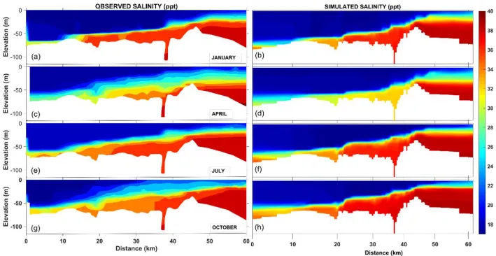
salinity and temperature processes profiles along the Strait are also examined. Figure 9 presents the
289
longitudinal salinity profiles of the Istanbul Strait for four different months, namely January, April,
290
July, and October. According to this figure, dispersion and distribution of salinity in the model
291
substantially agrees with the in-situ observations. Stratification in the Strait clearly reveals itself in
292
salinity profiles, such that the upper and lower flow layers can easily be distinguished. Normally,
293
upper zones are less saline, around 18-20 ppt, and deeper zones are more saline, around 38-40 ppt.
294
This is because, the upper layer originates from Black Sea fed by less saline sources such as the
295
Danube River, while the source of the lower layer is saline waters of Marmara, Aegean, and
296
Mediterranean Seas. It can be seen from the model results as well as observations that when the
297
flowrate of the upper layer increases, thickness of this layer with the less saline water mass (blue in
298
300
301
Figure 9. Salinity profiles of observed (a) and modeled (b) in January, observed (c) and modeled (d) in April, observed (e) and modeled (f) in July, and observed (g) and
302
304
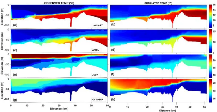
Another conspicuous feature of the Strait is the variation seawater temperature in vertical.
305
Figure 10 gives the longitudinal temperature profiles of the Strait, respectively in January, April, July,
306
and October. This figure also involves the model results as well as the measured temperature profiles.
307
The most imperative feature of the Strait, stratification, is also clearly represented by the numerical
308
model from the temperature viewpoint. Although a general agreement between the model results
309
and the measured data can be assessed, it is seen that the performance of the numerical model for
310
modelling the temperature profiles is not as effective as the salinity modeling. The potential reason
311
is that more complicated atmospheric effects (such as atmospheric cooling and warming) are engaged
312
in the temperature modeling on the contrary of salinity, which is mostly governed by the
313
oceanographic/mareographic parameters. Nevertheless, the profiles of the stratified temperature
314
structure can generally said to be captured by the numerical model results, even though it is not as
315
accurate as salinity profiles. For instance, in January and April, upper layer is colder than lower layer,
316
and in the July and October vice versa. Both conditions are exhibited in the numerical model within
317
a fair approximation. A visible drawback in the model is that, thickness of the intermediate layer
318
could not always be properly modeled. Especially in the July results, this defect is observed.
319
Irrespective of the drawback, it can be said that observed temperature profiles are modelled with a
320
fair agreement.
321
323
324
Figure 10. Temperature profiles of observed (a) and modeled (b) in January, observed (c) and modeled (d) in April, observed (e) and modeled (f) in July, and observed (g)
325
327
4. Discussion
328
In this study, Istanbul Strait, one of the most complicated waterways in the world with its
329
meandering shape, stratified structure, and hydraulic control process, is numerically modelled. The
330
main objective of the study is to model the hydrodynamic and hydrographic constitution of the Strait,
331
as well as assessing the most sensitive hydrodynamic parameters to reach a successful solution.
332
Three different methods are employed for calibration of the model by comparing the in-situ
333
measured flowrates of upper and lower layers at the North and South parts of the Strait with the
334
numerical model results. Among the employed methods, Levenberg-Marquardt Algorithm (PEST
335
method) came out to be the best to calibrate the model, not only due to the closest agreement between
336
the measurements and the model, but also with the physically consistent values of the input
337
parameters attained as the end-product of the calibration process. With the mentioned method used,
338
correlation between numerical model results and observations got higher. Especially in the Northern
339
section of the Strait, the method was perceptibly successful.
340
Sensitivity analysis showed that among the 17 input parameters, the following five has the most
341
prominent effect on the results: (1) Spatial Low-Pass Filter Coefficient, (2) Horizontal Eddy Viscosity,
342
(3) Prandtl-Schmidt Number, (4) Slope in log-log Spectrum, and (5) Manning Roughness Coefficient.
343
Apart from the flowrate results of the upper and lower layers, salinity and temperature profiles
344
of the stratified flow in the Strait were assessed by the numerical model, in comparison with the
in-345
situ measurements. This latter comparison served as a means of validation of the numerical model.
346
Modeled salinity profiles came out to be another prospering output of this study. Beside the
347
stratification of the Strait, salinity values and layer thicknesses are modeled in good agreement with
348
the measurements, such that modeled and observed salinity profiles closely resembled each other.
349
When it comes the temperature profiles, stratification and seasonality variations were seen to be fairly
350
represented in the numerical model results. Although the thickness of the intermediate cold layer
351
was not accurately estimated by the model results, general temperature profiles of the model were
352
seen to be in accord with observed profiles. Choosing calibration and validation dataset very different
353
is one of the unique feature of our study. Obviously if the calibration framework includes the
354
observed temperature as part of the objective function, the model simulation performance on
355
temperature profiles will substantially increase. This is an ongoing modelling effort and will be the
356
topic of a subsequent study.
357
With this numerical modelling study, it was clearly seen that the robustness of the model is
358
depending on the sufficient representation of the boundary and initial conditions, as well as the
359
accurate water level inputs which are the main forcing factor of the flow. Stratification phenomena
360
can only be modeled with properly assigning the stratified boundary and initial conditions, as was
361
done in the present study.
362
In future studies, temporal and spatial domains of the model could be extended in order to
363
model the Strait in a more proper way, preferably with a higher grid resolution. As such, the
364
agreement of hydrodynamic and hydrographic outputs between model and the observations could
365
get better in these future studies, with which estimations on the effect of climate change on the
366
delicate flow regime of the Istanbul Strait can possibly be modelled.
367
Author Contributions: conceptualization, M.M.K. and M.C.D.; methodology, M.M.K. and M.C.D.; software,
368
M.M.K. and M.C.D.; validation, M.M.K., M.C.D. and V.S.O.K.; formal analysis, M.C.D. and V.S.O.K.;
369
investigation, M.M.K. and V.S.O.K.; resources, M.M.K. and V.S.O.K.; data curation, M.M.K. and M.O.; writing—
370
original draft preparation, M.M.K., M.C.D., V.S.O.K and M.O.; writing—review and editing, M.C.D. and
371
V.S.O.K.; visualization, M.M.K., M.C.D. and V.S.O.K.; supervision, M.O.
372
Funding: This research was funded by Istanbul Technical University, grant number 38420. The second author
373
(MCD) is supported by Turkish Scientific and Technical Research Council (TÜBİTAK grant 118C020)
References
376
1. Çeçen, K.; Bayazıt, M.; Sümer, M.; Güçlüer, Ş.; Doğusal, M.; Yüce, H. İstanbul Boğazı’nın Hidrolik ve
377
Oşinografik Etüdü (The Hydraulic and Oceanographic Survey of Istanbul Strait); Istanbul Technical University:
378
Istanbul, 1981;
379
2. Bayazıt, M.; Sümer, M. İstanbul Boğazı’nın Hidrolik ve Oşinografik Etüdü - 2 (The Hydraulic and
380
Oceanographic Survey of Istanbul Strait - 2).pdf 1982, 23.
381
3. Sumer, B.M.; Bakioglu, M. Sea-Strait Flow With Special Reference To Bosphorus. 1981.
382
4. Latif, M.A.; Ö zsoy, E.; Oguz, T.; Ü nlüata, Ü . Observations of the Mediterranean inflow into the Black
383
Sea. Deep Sea Res. Part A. Oceanogr. Res. Pap.1991, 38, S711–S723.
384
5. Özsoy, E.; Beşiktepe, Ş.; Latif, M.A. Türk Boğazlar Sistemi’nin Oşinografisi (Oceanography of the
385
Turkish Strait System). 2000.
386
6. Falina, A.; Sarafanov, A.; Özsoy, E.; Utku Turunçoğlu, U. Observed basin-wide propagation of
387
Mediterranean water in the Black Sea. J. Geophys. Res. Ocean.2017, 122, 3141–3151.
388
7. Sur, H.I.; Ö zsoy, E.; Ü nlüata, Ü . Boundary current instabilities, upwelling, shelf mixing and
389
eutrophication processes in the Black Sea. Prog. Oceanogr.1994, 33, 249–302.
390
8. Oguz, T.; Ö zsoy, E.; Latif, M.A.; Sur, H.I.; Ü nlüata, Ü . Modeling of Hydraulically Controlled Exchange
391
Flow in the Bosphorus Strait. J. Phys. Oceanogr.1990, 20, 945–965.
392
9. Farmer, D.M.; Armi, L. Maximal two-layer exchange over a sill and through the combination of a sill
393
and contraction with barotropic flow. J. Fluid Mech.1986, 164, 53–76.
394
10. Armi, L.; Farmer, D.M. Maximal two-layer exchange through a contraction with barotropic net flow. J.
395
Fluid Mech.1986, 164, 27–51.
396
11. Armi, L. The hydraulics of two layers with different densities. J. Fluid Mech.1986, 163, 27–58.
397
12. Dorrell, R.M.; Peakall, J.; Sumner, E.J.; Parsons, D.R.; Darby, S.E.; Wynn, R.B.; Ö zsoy, E.; Tezcan, D. Flow
398
dynamics and mixing processes in hydraulic jump arrays: Implications for channel-lobe transition zones.
399
Mar. Geol.2016, 381, 181–193.
400
13. Beşiktepe, Ş.T.; Sur, H.I.; Özsoy, E.; Latif, M.A.; Oǧuz, T.; Ü nlüata, Ü . The circulation and hydrography
401
of the Marmara Sea. Prog. Oceanogr.1994, 34, 285–334.
402
14. Ozsoy, E.; Latif, M.A.; Besiktepe, S.; Ç etin, N.; Gregg, M.C.; Belokopytov, V.; Goryachkin, Y.; Diaconu,
403
V. The Bosporus Strait: Exchange Fluxes, Currents and Sea-Level Changes. Nato Sci. Ser. 2 Environ. Secur.
404
1998, 47, 1–28.
405
15. Gregg, M.C.; Ö zsoy, E.; Latif, M.A. Quasi-steady exchange flow in the Bosphorus. Geophys. Res. Lett.1999,
406
16. Gregg, M.C.; Ö zsoy, E. Flow, water mass changes, and hydraulics in the Bosphorus. J. Geophys. Res.2002,
408
107.
409
17. Güler, I.; Yüksel, Y.; Yalçiner, A.C.; Ç evik, E.; Ingerslev, C. Measurement and evaluation of the
410
hydrodynamics and secondary currents in and near a strait connecting large water bodies-A field study.
411
Ocean Eng.2006, 33, 1718–1748.
412
18. Yuksel, Y.; Ayat, B.; Nuri Ozturk, M.; Aydogan, B.; Guler, I.; Cevik, E.O.; Yalçiner, A.C. Responses of the
413
stratified flows to their driving conditions-A field study. Ocean Eng.2008, 35, 1304–1321.
414
19. Aydoǧan, B.; Ayat, B.; Ö ztürk, M.N.; Ö zkan Ç evik, E.; Yüksel, Y. Current velocity forecasting in straits
415
with artificial neural networks, a case study: Strait of Istanbul. Ocean Eng.2010, 37, 443–453.
416
20. Jarosz, E.; Teague, W.J.; Book, J.W.; Beşiktepe, Ş. Observed volume fluxes in the Bosphorus Strait.
417
Geophys. Res. Lett.2011, 38, n/a-n/a.
418
21. Altiok, H.; Kayişoğlu, M. Seasonal and interannual variability of water exchange in the Strait of Istanbul.
419
Mediterr. Mar. Sci.2015, 16, 644–655.
420
22. Ozsoy, E.; Cagatay, M.N.; Balkis, N.; Balkis, N.; Ozturk, B. The Sea of Marmara - Marine Biodiversity,
421
Fisheries, Conservation and Governance; 2016; ISBN 9789758825349.
422
23. Akay, O. Hydrodynamic Simulation of the Bosphorus, Istanbul Technical University, Institute of Science
423
and Technology, 2002.
424
24. Öztürk, M.N. İstanbul Boğazı’nın Hidrodinamiği ve Sayısal Modellenmesi (Hydrodynamics of the
425
Istanbul Strait and its Numerical Model), Yildiz Technical University, 2010.
426
25. Sözer, A. Numerical Modeling of the Bosphorus Exchange Flow Dynamics, Middle East Technical
427
University, 2013.
428
26. Sözer, A.; Ö zsoy, E. Modeling of the Bosphorus exchange flow dynamics. Ocean Dyn.2017, 67, 321–343.
429
27. Sannino, G.; Sözer, A.; Ö zsoy, E. A high-resolution modelling study of the Turkish Straits System; Ocean
430
Dynamics, 2017; Vol. 67; ISBN 1023601710.
431
28. Armi, L.; Farmer, D.M. The Internal Hydraulics of the Strait of Gibraltar and Associated Sills and
432
Narrows. Oceanol. Acta1985, 8, 37–46.
433
29. Bruno, M.; Chioua, J.; Romero, J.; Vázquez, A.; Macías, D.; Dastis, C.; Ramírez-Romero, E.; Echevarria,
434
F.; Reyes, J.; García, C.M. The importance of sub-mesoscale processes for the exchange of properties
435
through the Strait of Gibraltar. Prog. Oceanogr.2013, 116, 66–79.
436
30. Koşucu, M.M. Three-Dimensional Hydrodynamic Model of the Istanbul Strait, Istanbul Technical
437
University, Institute of Science and Technology, 2016.
438
31. Sur, H.İ.; Okuş, E.; Güven, K.; Yüksek, A.; Altiok, H.; Kıratlı, N.; Ünlü, S.; Taş, S.; Aslan Yılmaz, A.;
Yılmaz, N.; et al. Water Quality Monitoring: Annual Report (2003); Istanbul, 2004;
440
32. Delft3D user manual Simulation of multi-dimensional hydrodynamic flow and transport phenomena,
441
including sediments 2014, 684.
442
33. Cornelissen, S. Numerical Modelling of Stratified Flows Comparison of the σ and z coordinate systems.
443
2004, 1–94.
444
34. Lesser, G.R.; Roelvink, J.A.; van Kester, J.A.T.M.; Stelling, G.S. Development and validation of a
three-445
dimensional morphological model. Coast. Eng.2004, 51, 883–915.
446
35. Huang, W.; Spaulding, M. Modeling horizontal diffusion with sigma coordinate system. J. Hydraul. Eng.
447
1996, 122, 349–356.
448
36. Doherty, J. PEST: Model Independent Parameter Estimation. Fifth Edition of User Manual; Watermark
449
Numerical Computing: Brisbane, 2005;
450
37. Doherty, J. Calibration and Uncertainty Analysis for Complex Environmental Models; Watermark Numerical
451
Computing: Brisbane, Australia, 2015; ISBN 978-0-9943786-0-6.
452
38. Doherty, J. Model-Independent Parameter Estimation(Part I); 6th ed.; Watermark Numerical Computing,
453
2016;
454
39. Hansen, N.; Ostermeier, A. Completely derandomized self-adaptation in evolution strategies. Evol.
455
Comput.2001, 9, 159–195.
456
40. Hansen, N.; Ostermeier, A. Adapting arbitrary normal mutation distributions in evolution strategies:
457
the covariance matrix adaptation.; 2002.
458
41. Dey, S. Fluvial hyrodynamics: Hydrodynamic and sediment transport phenomena; Springer: Berlin, Germany,
459
2014; ISBN 978-3-642-19061-2.
![Figure 1. Study area and hydrographic observation stations in the Istanbul strait [31]](https://thumb-us.123doks.com/thumbv2/123dok_us/7928084.1316394/3.595.104.488.483.747/figure-study-area-hydrographic-observation-stations-istanbul-strait.webp)

![Table 1. Sensitivity analysis results using PEST tool [37] [38]](https://thumb-us.123doks.com/thumbv2/123dok_us/7928084.1316394/8.595.75.519.210.472/table-sensitivity-analysis-results-using-pest-tool.webp)