Article
Computational simulation of PT6A gas turbine engine
operating with different blends of biodiesel: A
transient-response analysis
Camilo Bayona-Roa1,2,*, J.S. Solís-Chaves1 , Javier Bonilla1, A.G. Rodriguez-Melendez1and Diego Castellanos1
1
2
3
4
5
6
7
8
9
10
11
12
1 UniversidadECCI,Cra.19No.49-20,Bogotá111311,Colombia
2 CentrodeIngenieríaAvanzada,InvestigaciónyDesarrollo—CIAID,Bogotá111111,Colombia
* Correspondence:[email protected]
Abstract: Instead of simplified s teady-state m odels, w ith m odern c omputers, o ne c an s olve t he complete aero-thermodynamics happening in gas turbine engines. In the present article, we describe a mathematical model and numerical procedure to represent the transient response of a PT6A gas turbine engine operating at off-design conditions. The aero-thermal model consists of a set of algebraic and ordinary differential equations that arise from the application of the mass, linear momentum, angular momentum, and energy balances in each engine’s component. The solution code has been developed in Matlab-Simulink®using a block-oriented approach. Transient simulations of
the PT6A engine start-up have been carried out by changing the original Jet-A1 fuel with biodiesel blends. Time plots of the main thermodynamic variables are shown, especially those regarding the structural integrity of the burner. Numerical results have been validated against reported experimental measurements and GasTurb®simulations. The
computer model has been capable to predict acceptable fuel blends, such that the real PT6A engine can be substituted to avoid the risk of damaging it.
Keywords:Gas turbine engine; Two-spool turboprop engine; PT6A engine; Aero-thermal model; Matlab-Simulink; Bio-diesel; Start-up transient.
13
1. Introduction 14
The necessary thrust that is required for an aircraft to provide lift is commonly supplied by a heat engine. 15
In particular, a gas turbine engine can convert heat energy into mechanical energy by involving the flow of air 16
passing through several thermo-fluidic processes within its components. One of the most important features of 17
gas turbine engines is that, contrary to reciprocating engines, separate sections of the engine are devoted to the 18
intake, compression, combustion, power conversion, and exhaust processes. This also means that all processes are 19
performed simultaneously and that they are strongly coupled between them. Hence, the conceptual description of the 20
gas turbine engine’s response is complex; it involves the approximation from very different engineering disciplines: 21
Aerodynamics, Thermodynamics, Heat Transfer, Structural Analysis, Materials Science, and Mechanical Design. 22
Remarkably, in all those fields the mathematical modeling of a gas turbine engine is constructed by applying the 23
mass, energy, and momentum balances over the most representative solid and fluid elements of the engine. These 24
balances have to do with the air crossing through the gas turbine engine’s stages and its interaction with the rotatory 25
solid components. The overall result of this modeling process gives a set of several partial differential equations whose 26
solution is the spatial and temporal description of the air through the engine’s stages and the performance of the 27
engine. Since there are not any exact solutions due to the geometry complexity and temporal dependence, we rely 28
entirely on numerical methods to find an approximated numerical solution. 29
The level of numerical resolution of each component is also important: a great level of detail in the description 30
may also be computationally expensive. Selecting one or other may be based on the objectives of the simulation and the 31
given computational resources. In a turboprop engine modeling, for example, the complex geometric description of the 32
rotary components makes it hard to generate a full spatial solution, namely a discrete spatial mesh for Computational 33
Fluid Dynamics (CFD). Considering the dynamic rotatory movement of the components raises —even more— the 34
model complexity and the computational cost. Trying to couple the engine’s components in the CFD simulation is a 35
problem that may not be solvable with actual computational methods and power. 36
And that is our particular motivation in the present work: to simulate the overall engine performance. We are also 37
restricted by the computational resources at hand, which are a personal computer. These requirements typically lead 38
to neglect a very detailed spatial description of the airflow, preferring an integrated definition of each engine stage 39
to what is referred to as a lower-dimensional model. This approach defines space-averaged values at each engine’s 40
component, and the partial differential equations arising from the balance equations turn to ordinary differential 41
equations that can be solved numerically in an affordable way. The important aspect is that this spatially-simplified 42
approach is capable to represent the engine’s operation giving accurate physical solutions that arise from the balance 43
equations. 44
Precisely, we are interested in computational simulations capable of representing the PT6A turboprop gas turbine 45
engine performance when a change in the operating fuel occurs. Specifically, the evaluation of the transient state of 46
the engine at the start-up procedure, when the temperature in the burner reaches its maximum and can significantly 47
affect the combustion chamber. Testing a gas turbine operating with fuel compositions is costly and time-consuming, 48
but also leads to performance degradation of the manufactured engine. Instead, the tests that can be achieved with 49
computational models like [1–4] are inexpensive and fast when used for new designs, predicting the system’s integrity, 50
and calculating real-time responses. In this sense, a wide range of computer engines have been implemented: from 51
systematic models in [5–9], to the detailed component design of engine parts in [10–15]. Because of the previously 52
supported reasons, we opt for an integrated representation of the engine as an assembly of components to what 53
is commonly referred to as a Common Engineering Model (CEM). These components —inlet, fan, compressors, 54
combustion, turbine, shafts, and nozzle— are abstracted in the computational model as blocks —or objects—, having 55
connections between them and therefore, being able to model the various propulsion systems, such as multi-spool or 56
turbo-fan type of engines. 57
We restrict our survey to engine models based on physical descriptions of the engine components. Those range 58
from simulation tools used by the gas turbine production and control industry [16], steady and transient performance 59
simulations of power gas turbines in [17,18], and general gas turbine software such as DYNGEN [19], TERTS [20], 60
GSP [21], Gasturbolib [22], GasTurb®[23], among others. Academic research has exploited the architectures given by
61
Matlab-Simulink®[22], and Modelica®[24], where different engine types can be created in a visual interface approach.
62
However, most simulate the steady-state thermodynamic cycle of the engine, without describing the dynamic behavior 63
of the air that crosses the stages of the engine, and nearly all are linearized versions that do not work far from the 64
linearization point like when the engine operates with blends of biodiesel fuel. Some developed approaches solve the 65
non-linear version of the equations employing the Newton-Raphson methods that require the computation of the 66
Jacobian and may not converge to the actual numerical solution at all operating regimes. The particular methods that 67
we are interested in, are the ones that do not require an extensive iterative process to obtain the numerical solution of 68
the set of algebraic and differential equations. Those arrange the equations in such a way that the output values can be 69
obtained from the input variables. This is consistent with the flow of air through the engine components: the input 70
variables are referred to the entering flow conditions, while the output solved variables are the exiting flow. 71
The thermal performance prediction of gas turbine engines operating with biodiesel has barely been reported in 72
[25,26] using these computational techniques. The opposite is true for reciprocating engines operating with biodiesel 73
blends, for which performances and emissions predictions have been carried out. Simulated steady results for gas 74
turbine engines indicated that the modified lower heating value of the biodiesel fuel had a significant influence on 75
thrust, fuel flow and specific fuel consumption at every flight condition and all mixing ratio percentages. Those 76
preliminary results are encouraging and motivate research in engine technology advancements for substituting the 77
source of jet fuel from fossil-based fuel to biomass-based, which could reduce the environmental impact and energy 78
consumption. 79
Our computational approach to simulate the transient response of a gas turbine engine operating with blends of 80
been done. In contrast to those approaches, we consider the gas dynamics, which are the application of the mass, 82
momentum and energy balances at every component of the gas turbine engine. Especially at the compression and 83
turbine sections, where a stage-by-stage thermo-fluidic description is done for high-fidelity purposes. Another key 84
aspect of the present work has to do with the solution algorithms and the development of the model in a flexible 85
programming architecture, which makes it possible to create the specific configuration of the PT6A turboprop engine 86
but also enables the future extension of the engine model. We formulate each engine component using a separate 87
block, in which the mass, momentum and energy equations give the solution of the dynamical variables. The complete 88
engine is the composition of blocks resulting in a block diagram. Matlab-Simulink®offers the capability of coding
89
those blocks and connecting them to configure any gas turbine engine. It also gives the possibility of using a graphical 90
interface which is more user-friendly, but the relevant feature of this software is that it makes possible to generate 91
source code in C language to generate a much faster executable program. Block diagrams make also possible to link 92
the engine software to control devices, with the capability of driving input/output signals for data acquisition and 93
control. 94
The remaining parts of this article are organized in the following order. In Section2, the real operational gas 95
turbine engine is described: we reproduce a generic version of the Pratt-Whitney PT6A engine. Simultaneously, 96
we present the theoretical description of the thermodynamic processes occurring inside each engine’s components. 97
The simulation of different scenarios are given in Section3. The scenarios include the validation of our model with 98
the reported experimental data of the engine’s steady operation, the subsequent steady operation with blends of 99
biodiesel, and the transient engine response at the start-up procedure to determine the engine’s structural integrity 100
and deterioration when operating with blends of bio-diesel. Finally, in Section4some conclusions close the article. 101
2. The PT6A engine model 102
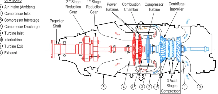
A generic version of the Pratt-Whitney PT6A-65 "Medium" engine, including the labeling of its parts, is displayed 103
in Fig.1. In general, gas turbine engines consist of: an air inlet, a compression section (including the compressor and 104
diffuser), a combustion section (combustion chamber), a turbine section, an exhaust section, and an accessory section 105
(for necessary systems). The theoretical description of the thermodynamic processes occurring in these components is 106
Brayton’s cycle. But the dynamic simulation of the engine’s behavior must account for non-equilibrium conditions, 107
which is the case of the start-up procedure of the engine. The Brayton’s model must, therefore, be complemented with 108
the actual design of the turbo-machinery of the engine’s stages. 109
We develop a gas-dynamical model for describing the thermo-fluidic phenomena present in each gas turbine 110
engine’s component. For doing so, we apply the fluid’s continuity balance for every component of the engine. 111
Especially those with transient mass storage, namely the combustion chamber where compressible effects of the air are 112
relevant, and for the coupling of mass fluxes between consecutive components. We also apply the fluid’s momentum 113
balance at the core flows in the compressor and turbine stages. Fluid’s energy balance accounts for the combustion 114
chamber heat addition and the compression and expansion processes. The mechanical energy equation is also applied 115
to the rotor stages, including the inertial and frictional loses terms of the rotor shaft, to model the mechanical coupling 116
between the moving components. Since our model focus on describing the primary flow-path components and avoids 117
the description of the structural behavior of the solid parts of the engine, which are not essential in the engine’s 118
operation, we also neglect the heat transfer between the solid metal components and the gas in the energy balance 119
equation. As reported in previous works such as [18], some other non-flow-path components affect the ability to 120
maintain the operation conditions, and accounting for them can be significant to obtain accurate simulations. This 121
is the case of the combustion model, the fuel system, or the external loads related to the propeller. Although we 122
acknowledge the importance of these systems, we exclude the engine-inlet or engine-outlet integration (to reproduce 123
the inlet and outlet flows), the engine-aircraft integration (to reproduce structural analysis), the engine-environment 124
integration (for adverse weather and pollution), and the control systems. 125
The application of these balances to the engine’s components results in a0-dimensional modelrepresenting the 126
operation at transient state. This "aero-thermal" model is usually confined to the normal operating range of the 127
engine, but in the present work is aimed to give the engine response at off-design operating conditions. A practical 128
approach to numerically solving the 0-dimensional model is to implement it in Matlab-Simulink®software [28], which
129
equations. Hence, we present the global block diagram of the governing equations in Fig.2, where the engine model is 131
represented at a component level. An extended explanation of each engine’s component, and how we represent it, 132
will be developed through the following paragraphs. Moreover, each component’s block diagram will be presented 133
through the detailed explanation of each sub-system. We list inputs, parameters, variables, and outputs for every 134
block diagram. 135
Figure 1.Cross section and stations of the Pratt-Whitney PT6A-65 engine.
2.1. Air inlet 136
One of the main characteristics of this gas turbine engine is that in most aircraft installations it is mounted 137
backward in the nacelle. This feature makes that the airflow inside the components of the engine is directed in the 138
same direction as the aircraft’s displacement. Another consequence is that the intake is located at the rear part of 139
the engine, and therefore, the air passes through the exterior of the aircraft (and the engine itself) before entering 140
to the intake. The PT6A-65 design cares for guiding the intake air to the engine using ducts that avoid facing the 141
exhaust gases: since the typical requirement is to provide laminar air into the compressor —so that, it can operate 142
at maximum efficiency—, the inlet duct changes smoothly from opposing the direction of the airflow to the axially 143
forward direction of the aircraft’s speed. 144
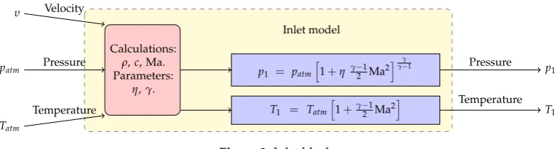
We define the inlet component as to be the intake air conditioner: even though our model is restricted to an 145
on-ground operation, with no rarefying processes of the atmospheric air entering into the engine, we extend the 146
possibility of the operation of the model duringin-flight operationconditions. This effect is modeled using the relations 147
for the pressure and temperature of the air which are presented in the block diagram of Figure3. In the model,patm, 148
andTatmare the atmospheric pressure and temperature, Ma=υ/cis the flight Mach number that relates the aircraft 149
speedυwith the speed of soundc=pγpatm/ρ. The quotient between specific heats of the air is denoted byγ, and 150
ηis the isentropic efficiency. We use the subscript 1 to label the thermodynamic variables of air at the inlet. Note 151
that when the engine is supposed to operate in the ground test bench, the model equates the inlet conditions to the 152
atmospheric conditionsp1=patm, andT1=Tatm.
153
2.2. Compression section 154
The compression section of the PT6A-65 gas turbine engine (used for aviation) consists of threeaxial stagesand 155
a singlecentrifugal stage, each considered to be a rise in the air’s pressure: the air flows from the inlet duct to the 156
low-pressure compressor, and then to the next two axial-flow stages before passing to the centrifugal stage. The axial 157
stages are composed by rotating blades calledrotors, and static blades calledstators. Those rotating stages move at 158
around 40000 Revolutions Per Minute (RPM) increasing the air’s pressure more than eight times the inlet’s pressure. 159
Input
data
Inlet.
Axial
compr
ession
stages.
Centrifugal compr
essor
.
Burner
.
Compr
ession
turbine.
Power turbine stages.
Compr
ession
section
rotating
shaft.
Power rotating shaft.
pat
m
,
Tat
m
,
u
,
˙
mf
,
M
l
,
ω
c
(
t
=
0
)
,
ω
p
(
t
=
0
)
p1
,
T1
p
i,T i,
˙
ma ,∑
3 i=
1
M
i
p2
,
T2
,
M
p3
,
T3
p
j,T j,M j,
˙
mg
,
j
=
1
p
j,T j,M j,
˙
mg
,
j
=
2,
3
ω
c
ω
p
Figure
2.
Flow
chart
of
the
PT6A-65
engine’s
Calculations:
ρ,c, Ma.
Parameters:
η,γ.
p1 = patm
h
1+η γ−21Ma2
i γ
γ−1
T1 = Tatm
h
1+γ−1
2 Ma2
i
Inlet model
υ Velocity
patm Pressure
Tatm
Temperature
Pressure p
1
Temperature
T1
Figure 3.Inlet block.
outwardly. This centrifugal section has a high-pressure rise, but since there can be several losses between centrifugal 161
stages, it is restricted to a single-stage before discharging the airflow. The air stream then leaves the centrifugal 162
compressor section via the diffuser, which is a section of the engine just before the combustion chamber that has the 163
function of preparing the air for the burning area so that it can burn uniformly and continuously. We neglect the 164
diffuser in our representation of the compression section of the engine. 165
Preliminary work to the modeling of the compressor has to do with the estimation of its geometry. In this sense, 166
we determine the compressor’s geometry by extracting most of the information from technical reports, as well as from 167
the engine’s manual [29]. Since the axial compression section geometry has been reported in [30] for a four-axial stages 168
PT6A-65 engine, we transcript the geometrical parameters for the first and last stages, but calculate the mean values of 169
the second and third stages of that compressor, and set those values as the second axial stage of our PT6A-65 axial 170
compressor model. The geometric parameters that we have processed for each axial stage geometry are presented 171
in Table1. In the case of the inner and external radius of the rotor blades, we determine those parameters from 172
cross-checking the engine’s manual schemes and the measured values from a disassembled engine. The geometry 173
model of the centrifugal compressor is completely defined with the rotor’s blade geometry, and the inlet’s and outlet’s 174
cross-sectional dimensions. Where the inner r1and outerr2 radio of the rotor are determined from the engine’s
175
technical report, being 92 mm and 117 mm, respectively. 176
Table 1.Processed values of aerodynamic and geometric parameters for the axial compressor stages.
Blade Symbol 1st-stage rotor 2nd-stage rotor 3th-stage rotor
Inlet air angle, deg. αl 61.5 59.8 58.0
Exit air angle, deg. αt 54.4 48.9 42.0
Inlet metal angle, deg βl 56.8 57.85 57.1
Exit metal angle, deg. βt 50.5 43.5 36.2
Inner radius, mm. r0 72 76 80
Outter radius, mm. r 100 96 92
The overall compression stage is defined from the compressor intake(p1,T1)to state 2, at the diffuser outlet
177
(p2,T2). Therefore, it spans the three axial stages, the centrifugal stage, and the diffuser of the PT6A-65 engine. In
178
the present approach, we formulate the mass, momentum, and energy balance equations over each sub-stage of the 179
compressor to create a physically-detailed model. Knowledge of the inlet (upwind) conditions of the air, such as 180
temperature and pressure, as well as the rotational speed of the engine’s rotating shaft, are required. We also demand 181
the knowledge of the geometry of the compressor at each stage: since each compression section is composed of 182
successive stages of rotating blades (rotors) and stationary guide vanes (stators), we analyze at each rotor-stator stage 183
the transmission of the shaft’s mechanical energy into the air’s fluid energy and compose the complete compressor 184
performance by adding the multiple successive compression stages. 185
For simplicity, we assume that the compressor’s blades are thin, rather than having the complete airfoil cross-shape 186
geometry. This supposition is acceptable since in the PT6A-65 engine those are constructed of sheet metal. In the case 187
of the axial compressor, we analyze a singlei−th stage, where a rotor precedes a stator, and consider the same hub 188
radius for the rotor as for the stator. We also make this supposition for the shaft radius at each axial stage. Nevertheless, 189
we consider different cross areas between consecutive compression stages, such that the axial component of velocity 190
can be calculated to conserve mass: in the case of the multistage axial-flow compressor, the blades of each successive 191
cross-section of only one stator and rotor blade as it moves vertically, knowing that the next rotor blade passes shortly 193
thereafter. This is the well-known cascade two-dimensional approximation of turbomachinery analysis, and which 194
configures our control volume. 195
We aim to calculate the variation in the air’s enthalpy originated by the rotor’s torque. To do this, we apply 196
a simplified analysis of the fluid’s dynamics of the air occurring through the blade: thevelocity triangle. With this 197
approach, no component map representations or error relationships for the guesses of the unknowns are required and 198
therefore, no convergence issues of the numerical solution are found. Instead, direct physical solutions are encountered 199
for each component with the corresponding avoidance of convergence problems. To do this, the axial speed of the 200
airflow viacan be measured at the inlet section, such that the volume flow rate can be calculated in terms of the 201
cross-sectional area. Another possibility is to know the inlet air angle (presented in table1), such that the axial velocity 202
is calculated from the velocity triangle. To evaluate the torque on the rotating shaft, we use the angular momentum 203
balance that states that the total momentum in the shaftMis equal to the change between the angular momentum of 204
the flow that crosses the surfaces of the control volume. This change is only related to the tangential velocities of the 205
air given by the velocity triangle analysis. 206
In our model, we consider irreversible losses in the compression stages and therefore, the include a mechanical 207
efficiencyηthat implies a gap between the shaft power and the power delivered to the air. We suppose a quasi-static 208
and polytropic process in which the increment of energy in the air is given by the addition of mechanical power. 209
Indeed, the temperature rise inside the axial compression stage is calculated by applying the energy balance in 210
the control volume. The pressure ratioΠ(or net pressure head) induced by the compressor is calculated with the 211
polytropic process relation knowing the temperature variation of the air and the polytropic constant of the gasn. The 212
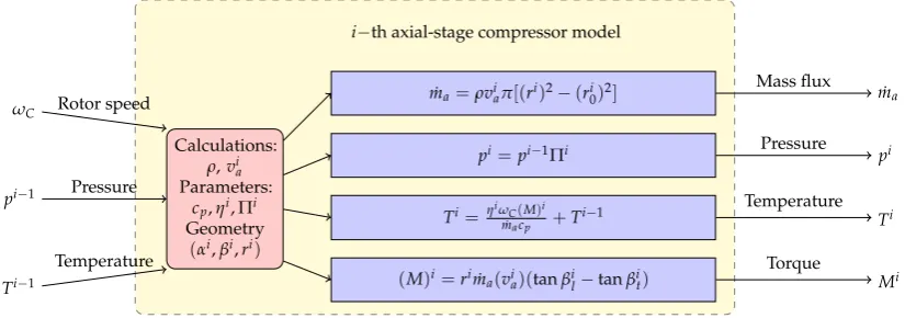
previous exposition is demonstrated in the block diagrams of Figures4and5. 213
For the centrifugal compressor, we consider that the circumferential cross-sectional area can be defined by the 214
radius and the width of the bladeb. We also suppose that the flow is defined completely in the normal direction(v1)n 215
and therefore, the normal velocity at the outlet of the blade can be calculated with the conservation of mass. 216
Calculations:
ρ,via Parameters:
cp,ηi,Πi
Geometry
(αi,βi,ri)
˙
ma=ρviaπ[(ri)2−(ri0)2]
pi=pi−1Πi
Ti=ηiωC(M)i ˙
macp +T i−1
(M)i=rim˙
a(via)(tanβil−tanβit) i−th axial-stage compressor model
ωC Rotor speed
pi−1 Pressure
Ti−1
Temperature
Mass flux ˙
ma
Pressure
pi
Temperature
Ti
Torque
Mi
Figure 4.Axial stages compressor block.
2.3. Burner 217
The PT6A-65 burner is mainly characterized by the split in the amount of compressed air that is used for 218
maintaining the combustion: only a fraction of the air entering in the burner reacts with the fuel, while most of the 219
compressed air is used for cooling purposes. The geometrical shape of the burner chamber is an annulus. In this 220
sense, the overall volume is hard to be determined and we have approximated its value from measurements of the 221
disassembled engine’s burner to be around 0.028 m3.
222
Inside the burner, the fuel and the air are separated apart before the flame: combustion with the liquid fuel 223
is performed by the injection of the fuel inside the air stream. Scattering of the fluid into fine droplets leads to the 224
convection and final evaporation of the liquid inside the compressed air-stream. This mixture is a steady non-premixed 225
stream of air-fuel before the full combustion reaction takes place inside the burner. Buoyant mechanisms, but mostly 226
Calculations:
ρ,
(v1)n,(v2)n. Parameters:
cp,ηi,Π
Geometry
(α,β,r,b)
˙
ma=m˙a
p2=piΠ
T2=η i
ωCM
˙
macp +T i
M=r2m˙a(v2)t−r1m˙a(v1)t Centrifugal compressor model ˙
ma Mass flux
ωC Rotor speed
pi Pressure
Ti
Temperature
Mass flux ˙
ma
Pressure p
2
Temperature
T2
Torque
M
Figure 5.Centrifugal compressor block.
the compression section) maintain the combustion process in the flame. The reaction rate and the products of the 228
combustion (exhaust gases) depend on the quality of the air-fuel mixture occurring before the flame. 229
The combustion quality is automatically controlled by thefuel control systemthat fixes the amount of injection; 230
this control is set by default for the Jet-A1 fuel. We neglect the fuel control in our present approach since we aim to 231
investigate the response of the engine to different blends with biodiesel. The change in the physical properties of 232
the fuel affects its spraying as it passes through the fuel injectors in the combustion chamber. This has effects on the 233
maximum temperature inside the fuel chamber at the start-up of the engine. In this sense, the starting procedure has 234
to be designed to be rigorous and must be established for each new operating fuel. For all the above, computational 235
simulation of the particular gas turbine engine’s performance is proposed as a predictive tool for the engine operation, 236
which allows determining the operation variables when the change in the composition of the fuel occurs. This, with a 237
low cost, and without risking the operation of test engines. 238
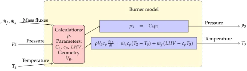
Our approach to model the burner’s combustion phenomena is simple and follows previous approaches like 239
[27]. The net power of the gas turbine engine is related to the amount of fuel that is burned inside the burner: the 240
heat added to the air-stream is calculated from the energy balance inside the burning chamber, whereLHVis the Low 241
Heating Value of the fuel that represents the amount of energy that is delivered in the combustion process (accounting 242
for the steam boiling in the liquid fuel). This is depicted in the block diagram of Figure6. 243
Note that the amount of chemical energy that is transferred to the air (which is later transformed to mechanical 244
energy in the turbine) depends on the type of fuel used, and this is completely characterized by the fuel flow rate 245
and its lower heating value. The burner also works as an accumulator of mass, where the temporal change of the 246
thermodynamic conditions of the air inside the burner is related to the amount of fuel ˙mf, the incoming airflow rate 247
˙
ma, the exhausting rate flow of gasses ˙mg, and the volume of the chamberVB. Note that the fuel flow is the input 248
specification for the fuel burner model, not the Fuel-to-Air Ratio (FAR) or the combustion temperature. The pressure 249
drop across the burner has also been adopted from [27], with the loss coefficientCb ≤1, depending on the square 250
mass flow rate. 251
Calculations:
ρ.
Parameters:
Cb,cp,LHV. Geometry
VB.
Burner model
p3 = Cbp2
ρVbcpdTdt3 =m˙acp(T2−T3) +m˙f(LHV−cpT3)
˙
ma, ˙mf, ˙mg Mass fluxes
p2 Pressure
T2
Temperature
Pressure p
3
Temperature
T3
2.4. Turbine section 252
The air stream leaves the burner with the addition of heat from the combustion and flows through several turbine 253
stages. The first turbine stage is a single-stage axial turbine that powers the compression section synchronously 254
rotating at 40000 RPM via theengine spool, or common shaft. From measurements of the disassembled engine spool, 255
we determine an overall mass moment of inertia of the engine spool of about 0.12 kg m2. 256
In the PT6A-65, the hot air flows then into thepower turbines, which are composed by two axial stages that turn at 257
about 30000 RPM, and that are connected to the main shaft that drives the propeller (or load). We also determine that 258
the mass moment of inertia of the main shaft is 0.06 kg m2. The air is discharged next to the exhaust, and then to the 259
atmosphere, where the air recovers its original free-stream conditions. 260
The turbine process is defined from the state 3 at the combustion chamber outlet(p3,T3)to state 4, at the engine
261
outlet(p4,T4). This means that the expansion ratio of the gas is known for the turbine section. Indeed, knowing the
262
expansion ratioΠjof thej−th stage, one can model each turbine stage as a polytropic expansion process where the 263
pressure and temperature of the air at the discharge can be calculated straightforwardly. 264
The temperature drop is then used to calculate the retrieved mechanical power inside the turbine. Again, we 265
suppose an irreversible process efficiency between the fluidic and the mechanical power, such that the extracted 266
torque at each axial stage of the turbine differs from the change in the angular momentum of the air inside the turbine. 267
Similarly to the axial flow compressor analysis, an accurate model of the turbine performance can be derived from a 268
detailed computation of the aerodynamics of the flow over the individual blade elements. The distinctive feature of 269
the turbine is that the mass flow rate of gases through the turbine section depends on the expansion work: we use the 270
angular momentum balance to obtain the mass flow of gases through the turbine stage, and therefore, the axial term of 271
the air velocity. The turbine relations are presented in the block diagrams of Figures7and8. 272
Calculations:
ρ,vaj. Parameters:
cp,nj,Πj Geometry
(βj,rj)
˙
mg=vjaρπ (rj)2−r20
pj=p3/Πj
Tj=T3/ Πj
(nj−1)
nj
Mj=rjm˙
g(vja)(tanβjl−tanβjt)
Engine spool’s turbine model
ωc Rotor speed
p3 Pressure
T3
Temperature
Mass flux m˙
g
Pressure
pj
Temperature
Tj
Torque
Mj
Figure 7.Engine spool’s turbine block.
Calculations:
ρ,vaj. Parameters:
cp,nj,Πj Geometry
(βj,rj)
˙
mg=vjaρπ (rj)2−r20
pj=pj−1/Πj
Tj=Tj−1/ Πj
(nj−1)
nj
Mj=rjm˙
g(vja)(tanβjl−tanβjt)
Power turbine model ˙
mg Mass flux
ωp Rotor speed
pj−1 Pressure
Tj−1
Temperature
Mass flux m˙
g
Pressure
pj
Temperature
Tj
Torque
Mj
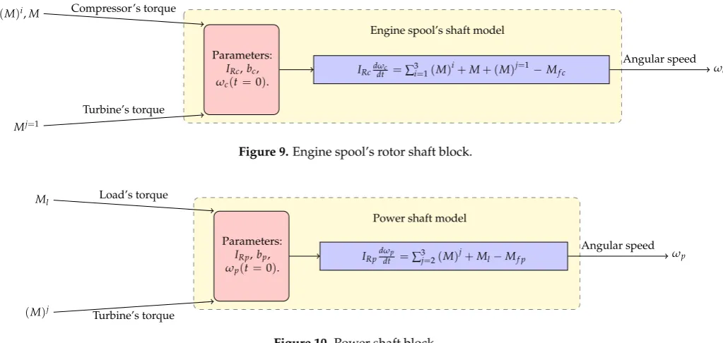
2.5. Rotating Shafts 273
The rotating shafts are modeled by applying the balance of angular momentum. We use the rigid body assumption, 274
and apply the momentum balance in the rotational motion, such that the acceleration power of the shaft must equal 275
the balance between turbine power, compression (or load) power, and parasitic powers. The angular momentum 276
balance applied to the engine spool, as well as the power rotating shaft is presented in the block diagrams of Figures9 277
and10, respectively. We defineIRto be the mass moment of inertia of the rotating shaft about its rotating axis,M 278
is each one of the torques applied to the shaft, andωis the angular velocity of the shaft which can be calculated in
279
terms ofω = Nπ/60, beingNthe revolutions per minute. The sum of power losses due to mechanical friction is 280
considered in the torqueMf, which is modeled using a loss-factorbthat is a function of the rotational speed of the 281
shaft, and its effect acting in the contrary-rotation sense. Following [27], we apply this mechanical losses model instead 282
of including a mechanical efficiency parameter of the shaft, since the numerical accuracy of the model is granted at the 283
idle condition or during the start-up procedure when the output power is negligible. 284
Parameters:
IRc,bc,
ωc(t=0).
IRcddtωc =∑3i=1(M)i+M+ (M)j
=1−
Mf c Engine spool’s shaft model
(M)i,M Compressor’s torque
Mj=1
Turbine’s torque
Angular speed
ωc
Figure 9.Engine spool’s rotor shaft block.
Parameters:
IRp,bp,
ωp(t=0).
IRpdωdtp =∑3j=2(M)
j+
Ml−Mf p Power shaft model
Ml Load’s torque
(M)j
Turbine’s torque
Angular speed
ωp
Figure 10.Power shaft block.
2.6. Compatibility conditions 285
Besides the physical description of each engine’s component, one must close the engine’s model coupling the 286
different components to what is referred to thecompatibility conditions. 287
The mass compatibility conditions are related to the conservation of the air mass flow rate. The inlet’s air mass 288
flow rate ˙mais calculated by knowing the inlet air angle at the first axial stage, such that the axial velocity can be 289
calculated knowing the rotational speed and the geometric parameters of the rotor blades. It has been explained 290
that ˙mais conserved among the stages of the compression section. Nevertheless, the mass compatibility condition 291
differs substantially when the air enters the burner: the exhaust gasses mass flow rate ˙mgis not only related to the 292
compressed air flow ˙mareacting with the mass flow of fuel ˙mf, but the exhaust gasses depend on the flow through the 293
turbine section and the engine’s exhaust. Here the compatibility condition is related to the mass flow rate resulting 294
from each turbine stage. Some further explanation about this compatibility condition will be taken in the next section. 295
On the other hand, the angular momentum compatibility condition is the balance of the torques applied for each 296
rotating shaft. Its readily understood that the rotation speed of the axial and centrifugal compressor stages matches 297
with the compressor’s turbine via the engine spool. In the same line, the velocity of the power turbines rotating shaft 298
matches the propeller’s shaft velocity through the reduction gear. 299
Finally, the energetic compatibility conditions are associated with the thermodynamic variables of the air at 300
the pressure and temperature conditions that it obtains at the stage immediately before. The overall compatibility 302
conditions become clear from the engine system’s block diagram depicted in Figure2. 303
3. Numerical Results 304
In this section, we present the numerical results for several simulation scenarios. As explained before, the 305
numerical solution of the set of algebraic and ordinary differential equations is achieved by Matlab-Simulink®. A
306
fourth-order Runge-Kutta numerical scheme for the temporal integration has been used for solving the differential 307
equations. A maximum integration step of 1ms has been used to guarantee the stability of the temporal solution. 308
The first scenario is the steady response of the engine which is intended to validate the computational model. Two 309
models have been set up, one with the present approach and the other one using GasTurb®[23]. We tested both models
310
to ensure the accuracy of the developed model at steady-state operation conditions, validating our results with the 311
engine test data and the commercial software simulation. Then, we solve the steady-state operation by using the 312
blends with biodiesel and compare our numerical results with the ones obtained with GasTurb. Finally, we address the 313
transient operation of the engine using the fuel blends, specifically at the start-up of the engine when the maximum 314
temperature can be reached. We suppose an on-ground operation in all scenarios so that the inlet velocity is set to zero. 315
3.1. Validation of the computational model 316
We first validate the computational model by considering the standard operation of the PT6A-65 engine reported 317
in the operation manual [29]. Those operation parameters are presented in Table2, where the International Standard 318
Atmosphere (ISA) conditions are set as the environmental conditions. We evaluate the stationary response of some 319
tracked variables (invariant in time): for the sake of validation, we track the stationary pressure, temperature, and 320
airflow at the stations of the engine. In Table3we list the experimental results that have been reported in the operation 321
manual for several stations of the engine, and that we use for the sake of comparisons. 322
Correspondingly with Section2, the geometrical parameters of the PT6A-65 motor described in that chapter are 323
implemented in our computational model. We fit some remaining geometric parameters so that we obtain the closest 324
numerical results to the ones reported in the operation manual: first, we determine the compression and expansion 325
ratios based on the experimental measurements. The overall compression ratio at the axial stages can be calculated 326
from the data in Table3to be 3.14 : 1 atm, while for the centrifugal compressor the compression ratio is around 2.56 : 1 327
atm. In this sense, we fit the centrifugal compressor’s anglesβ1andβ2to 40 and 38 degrees, respectively, such that the
328
centrifugal compressor gives rise to the pressure change. On the other hand, the expansion ratio for the compression 329
and power turbines are calculated to be 1 : 3.03 atm and 1 : 2.18 atm, respectively. We suppose an expansion ratio 330
of 1 : 1.47 atm for each stage of the power turbines section, and fit the blade’s angles to fulfill the mass flow rate 331
compatibility (conservation) condition between the different turbine stages. 332
Another quantity that the computational model requires is thenpolytropic index for each compression and expansion stage. We calculate that index by solving the logarithmic inverse expression for a polytropic process and accounting for the experimental PT6 engine operation. This is, considering the data in Table3, one can obtain the polytropic index with the expression
n= 1− logTf −logTi logpf −logpi
!!−1
.
Subscriptsiand f of the previous relation denote the initial and final condition of the gas in the polytropic process, 333
respectively. Then, the irreversible efficiency can be computed fromη=
γ−1
γ
/n−n1, where theγ =1.4 value 334
corresponds to the air. The gathered polytropic indexes and efficiencies for the PT6A-65 engine are presented in 335
Table4. Those values are set in the energy balances and polytropic processes of the compressor and turbine stages. 336
Table5presents the fitted aerodynamic and geometric parameters for all the turbine stages of the PT6A-65 engine 337
that have been processed. These parameters have been determined following the previously exposed ideas, from 338
cross-checking the engine’s manual schemes and the measured values from a disassembled engine, but mostly from 339
the fulfillment of the mass conservation requirement. The rotor blade airfoils, which are metal profiles followed and 340
Table 2.On-ground steady operation conditions using Jet-A1 fuel. Extracted from [29].
Standard conditions Value
Atmospheric temperature 288 K Atmospheric pressure 101352.9 Pa
LHV of Jet-A1 fuel 42.8 MJ/kg Jet-A1 fuel mass flow 0.062 kg/s Propeller’s load (at propeller’s shaft) 2684.51 N.m
Table 3.Temperatures and pressures for PT6A-65 engine at 850 shp and ISA standard conditions. Extracted from [29].
Station Location Temperature (K) Pressure (Pa)
0 Ambient 288 101352.9
1 Compressor Inlet 288.2 102042.4
1.5 Compressor Interstage 415.4 307506.2
2 Compressor Discharge 610.4 787381.28
3 Turbine Inlet 1212.1 770144.39
3.5 Interturbine 967.1 246142.8
4 Turbine Exit 811.5 113074
5 Exhaust 811.5 106179.3
is lost due to friction can be modeled by setting the bearing coefficientsbcandbpto 0.04 kg.m2/s and 0.05 kg.m2/s, 342
respectively, for the engine spool and power rotor shaft. We also model the pressure loss coefficient in the burner to be 343
Cb=0.95. These values arise from the numerical experiments that we performed guaranteeing the best approximation 344
of the computational model to the referenced values of the engine’s steady operation. 345
The simulated steady engine response is presented in Table6. In those results, we have assumed a constant 346
flow of Jet-A1 fuel, with a calorific power of 42.8 MJ/kg, and a constant propeller’s load torque of 2684.51 N.m. 347
We confirm a consistent physical behavior of the thermodynamic variables with the experimental reported ones. 348
Distinctively, the observed pressure at the discharge of the axial compressor stages is higher than the reported one. 349
This inaccuracy is countered by the centrifugal compression section, where the blade’s geometrical parameters are 350
fitted to give accurate results of the overall compression ratio. In this regard, fitting the compressor’s parameters 351
affects negatively the accuracy of the temperature at the discharge of the compression stage, but the energy balance 352
inside the combustion chamber counteracts this effect, and matches the stipulated temperature in the manual, with an 353
error of only 1.57%. Temperature and pressure variables at the expansion stages correspond well to the experimental 354
counterparts, mainly due to the possibility of fixing the expansion relation and the geometrical parameters of the 355
turbines. Given the previous exposition, we believe that the error is restricted to a low range such that it validates the 356
usage of the proposed model for predicting the engine response when new operating conditions are evaluated. 357
As explained before, we have also implemented the PT6 engine in the GasTurb software to validate our results: 358
we simulate the stationary operation of the engine using the Jet-A1 fuel and the same operating conditions that have 359
been listed in Table2. Since the GasTurb software has three different simulation levels: the basic thermodynamic 360
approach, an engine’s performance mode, and a more advanced engine’s performance simulation that considers the 361
specific geometry of the gas turbine engine, we have chosen the engine’s performance simulation. We have chosen 362
the default two-spools turboprop template that includes a booster and a compressor, the combustion chamber, and 363
the two expansion stations, but modified the template by inserting a high-pressure turbine in the engine’s spool, 364
and a low-pressure turbine in the power spool. The inputs for simulation in GasTurb have also been the polytropic 365
efficiencies of compressors and turbines, the atmospheric condition (temperature and pressure), the drop pressure in 366
the combustion chamber, the low heat value of the fuel, the maximum temperature in the combustion chamber, and 367
the pressure ratios in the compressor and turbine stations. The temperature and pressure results along the stations 368
of the PT6A-65 engine, together with the calculated relative error against the experimental measurements are also 369
presented in Table6. The comparisons between the developed model results and GasTurb demonstrate that although 370
there are some errors for certain stages in each model, the results from the present approach do not differ in accuracy 371
than those given by GasTurb. These results guarantee an acceptable resolution of the present approach and give the 372
Table 4.Polytropic index and efficiency gathered values for PT6A-65 engine.
Description Stages n η
Axial Compressor 1-1.5 1,496 0,862 Centrifugal compressor 2.5-3 1,693 0,698 Hot turbine expansion 3-3.5 1,247 0,693 Cold turbine expansion 3.5-4 1,291 0,789
Table 5.Fitted aerodynamic and geometric parameters of the turbine stages.
Blade 1st-stage rotor 2nd-stage rotor 3th-stage rotor
Inlet metal angle, deg 0 0 0
Exit metal angle, deg. 80 43 43
Inner radius, mm. 92 90 88
Outter radius, mm. 117 125 142
3.2. Stationary operation of the PT6A-65 using fuel blends 374
Once the present computational model has been validated, the following simulation scenarios are considered: we 375
evaluate the stationary operation of the PT6A-65 engine at both 100% of the fuel mass flow and 60% of the fuel flow, 376
meaning full throttle and idle operation, respectively. Since we aim to predict the engine’s response to the usage of 377
new hypothetical fuels, we vary the parameters related to the fuel’s modeling. In this sense, the standard Jet-A1 fuel 378
—kerosene— is mainly composed ofn−heptane and isooctane, which are hydrocarbons that possess between 8 and 16 379
carbon atoms per molecule, giving aLHVof around 42.8 MJ/kg (measured in experimental tests [31]). On the other 380
hand, the chemical composition of a biodiesel sample has been measured in [32] giving an approximatedLHVvalue 381
of 36.29 MJ/kg. Hence, the pure biodiesel retains a smaller amount of energy than conventional Jet-A1 fuel. 382
We simulate the engine operation with hypothetical blends of Jet-A1 with biodiesel. These fuel blends are 383
abbreviated as KB#, where "K" represents the Jet-A1 as the primary fuel, "B" represents the biodiesel as the secondary 384
fuel, and # is the mass fraction of biodiesel in the blend expressed in percentage. We establish a discrete range of mass 385
concentrations of biodiesel in Jet-A1 which are 3 in total: KB10, KB20, and KB30, and calculate theirLHVusing the 386
percent by mass of the mixture. The KB0 and KB100 represent the pure Jet-A1 and pure biodiesel fuels, respectively. In 387
the successive, we plot the simulation results for the operation with different blends of fuel, so that they are easily 388
comparable. Table7shows theLHVfor each blend and the notation to be used in the plots. 389
Figure11shows the air pressure through the engine stages. We observe a pressure rise at the compression section, 390
as well as an expansion process at the turbine stages. It is evident for both throttle operations that the maximum 391
pressure is located at the centrifugal compressor’s discharge (stage 2) and that there is a slight loss in this pressure at 392
the burner (stage 3). In the full-throttle case (right side of the figure), it can be observed that the pressure gap between 393
the Jet-A1 fuel and the pure biodiesel fuel is considerable, with an observable maximum pressure of 750 kPa and a 394
lower pressure of 610 kPa. In the case of the idle operation, there is a difference of 60 kPa between those fuels, with a 395
maximum pressure of 460 kPa and a minimum pressure of approximately 400 kPa. The fuel blends give results that 396
lay below some 5% of the Jet-A1 pressure range. In any case, the maximum values of pressure are related to the use of 397
the Jet-A1 fuel. This can be explained since it delivers the highest amount of power, which in turn is extracted by the 398
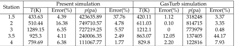
turbine stage and transferred to the compression section via the engine spool. 399
Table 6. Present and GasTurb simulation results. Stationary temperatures and pressures at different stations of the PT6A-65 engine. The relative error is calculated against the reported results in Table3.
Station Present simulation GasTurb simulation
T(K) Error(%) p(pa) Error(%) T(K) Error(%) p(pa) Error(%)
1.5 433.63 4.39 423635.89 37.76 420.11 1.12 318248 3.37
2 510.44 16.38 749710.57 4.78 611.03 0.10 814715 3.35
3 1289.15 6.35 727219.25 5.57 1212.1 0 773979 0.48
3.5 925.3 4.11 240006.35 2.49 863.07 12.05 137405 44.17
Table 7.Biodiesel blends.
Blend LHV(MJ/kg) Notation in Plots
KB0 42.8
KB10 42.14 ?
KB20 41.49 4
KB30 40.84 *
KB100 36.29
1 1.5 2 2.5 3 3.5 4
Stages 0
1 2 3 4 5 6 7 8
p
(P
a)
×105
1 1.5 2 2.5 3 3.5 4
Stages 0
1 2 3 4 5 6 7 8
p
(P
a)
×105
1 1.5 2 2.5 3 3.5 4 Stages
200 300 400 500 600 700 800 900 1000 1100 1200 1300
T
(K
)
1 1.5 2 2.5 3 3.5 4
Stages 200
300 400 500 600 700 800 900 1000 1100 1200 1300
T
(K
)
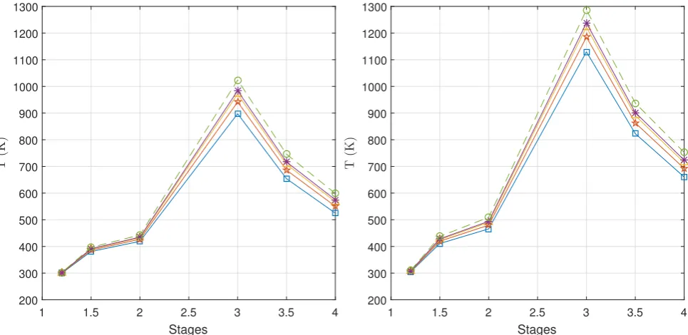
Figure 12. Temperature distribution along the engine stages. Results for the stationary engine operation with the 60% (left)and 100%(right)throttles.
Figure12displays the air temperature through the engine stages for the two different throttles. The temperature 400
results agree well with those reported in the manual: the maximum air temperature is observed at the burner discharge 401
(stage 3). In any scenario, the fuel that provides the highest temperature to the engine is the Jet-A1 fuel. For the 402
full-throttle operation there is a 200 K temperature difference in the burner between the Jet-A1 fuel and the pure 403
biodiesel fuel: the maximum temperature is given for the Jet-A1 fuel, reaching 1290 K, while the minimum temperature 404
of 1104 K is given by the biodiesel operation. The highest drop in temperature occurs at the compression turbine, 405
while the power turbines contribute lesser to the temperature reduction. It is also observed that the temperature 406
difference arising between the fuels at the burner is kept constant at the turbines discharge (stage 4). No important 407
temperature variation is observed for the biodiesel blends. Regardless of the fuel type, the temperature never exceeds 408
a value of 1050 K for the idle operation. 409
We also use GasTurb software to evaluate the engine performance running with biodiesel blends. Hence, we 410
display in Figure 13the pressure and temperature results obtained with the GasTurb model for the full-throttle 411
operation. We can observe that the GasTurb results for the different mixtures do not vary significantly. Although we 412
have imposed modified LHV values for each fuel, the GasTurb model seems not to be sensitive to these variations. 413
On the contrary, in our results, we can appreciate the variations in pressure and temperature that were commented 414
previously. 415
3.3. Transient operation of the PT6A-65 motor using fuel blends 416
Finally, we evaluate the start-up procedure of the engine with the fuel types that have been tested in previous 417
scenarios. The main goal is to identify problematic conditions during the engine start-up, which is the transient 418
procedure that can actually affect the engine’s integrity. The model is intended to run at zero speed and sea level 419
conditions, since the off-design operation of the engine are evaluated on a test bench. Being a two-spool turboprop, the 420
PT6A engine has been designed to be electrically started. The starter motor is represented in the engine simulation as 421
a constant rotational speed and starter torque. Hence, at the start up process, a simplified model with the imposition 422
of the rotational speed at the compression shaft and a constant torque load is implemented. The simulation is also 423
intended to run from idle to maximum power, but no shut down simulation is proposed since the objective is focused 424
on the combustion chamber’s limits. We configure the start-up procedure such that the compressor’s shaft starts 425
accelerating from its steady state condition toNc(t=0) =12000 RPM, which is the rotational speed that is provided 426
1 1.5 2 2.5 3 3.5 4 Stages
200 400 600 800 1000 1200 1400
1 1.5 2 2.5 3 3.5 4
Stages 1
2 3 4 5 6 7 8 9 10
5
Figure 13. GasTurb results. Temperature(left)and pressure(right)results for the stationary engine operation with the 100% throttle.
system) until the desired mass flow of air into the burner is granted. During the initial compression operation, no fuel 428
mass flow is injected into the burner. We consider that at a later instant(t=10)s, when the compressed air into the 429
burner stabilizes, the fuel is injected into the burner and ignited. The mass fuel flow is then gradually increased until 430
the desired throttle is reached at(t=tf). All the start-up procedure is considered to undergo with a constant torque 431
at the propeller’s shaftMl =2684.51 N.m. 432
We aim to evaluate the start-up procedure of the PT6A-65 engine with both 100% and 60% of throttle. The results 433
for the operation with fuel blends are displayed similarly as for the stationary operation. We present comparisons of 434
some important variables, such as the air pressure at the compressor discharge and the air temperature inside the 435
burner. It is noticeable that the start-up procedure converges to the steady-state operation. 436
Figure14shows the transient pressure results at the compression stage for the two different throttles. It can be 437
observed that the pressure in the compressor’s discharge undergoes an initial equilibrium when the engine spool is 438
started, reaching a compression ratio below of 1.5 : 1 atm. At(t=10)s, when the fuel is ignited, a sudden increment 439
of the compression ratio of around 2 : 1 atm is noticed for all fuels and throttles. In the case of the 60% throttle, the 440
pressure stabilizes from this instantaneous peak, but a pressure increasing delay for the full throttle case is noticeable, 441
reaching lately the reported 8 : 1 atm compression ratio. There is not a significant pressure fluctuation related to the 442
fuel blends: it can only be appreciated a moderate increment for the full throttle and the biodiesel fuel than for the 443
blends and Jet-A1 fuel. 444
The transient temperature inside the burner is presented in Figure15for the two different throttles. We observe a 445
slight increment in the temperature at the initial compression operation. Then, the fuel intake generates a temperature 446
peak in the combustion chamber, which in all scenarios is the maximum temperature that is reached during the 447
complete operation of the engine. Since the initial fuel flow is the same for both throttle scenarios, the maximum 448
temperature in the engine does not vary. Instead, it only depends on the fuel blend, where the maximum temperature 449
of 1300 K inside the burner is obtained with the Jet-A1 fuel, and the minimum of around 1100 K, approximately, is 450
obtained with the pure biodiesel. This is explained by the relatively smaller LHV of the biodiesel, which affects the gas 451
turbine combustion. After this critical instant, the temperature stabilizes at around 1000 K for the idle operation, with 452
fluctuation slightly greater than 100 K between the JetA1 and the biodiesel fuel. On the other hand, the temperature in 453
the full-throttle scenario increases gradually until the steady-state of 1290K is reached at about 40 s. 454
The first remark up to this point is that temperature controls have not been implemented in the present model. 455
0 10 20 30 40 50 t (s)
0 1 2 3 4 5 6 7 8
p2
(P
a)
×105
0 10 20 30 40 50
t (s) 0
1 2 3 4 5 6 7 8
p2
(P
a)
×105
Figure 14. Transient pressure at the compressor’s discharge. Results for the start-up operation with the 60%(left)and 100%(right)throttles.
present computer engine model we can compare the start-up operating temperature against the reference given by the 457
engine test data, which is the limit for structural integrity reasons and shutdown limit. In this sense, the standard 458
1300 K temperature limit [29] is not reached by any off-design operational scenario. The tests of the engine operation 459
with biodiesel blends show that the maximum temperature is lesser than 1220 K, which is acceptable for structural 460
reasons of the engine. However, in the real engine operation, the fuel is introduced by the fuel control system. Since 461
the accumulation of unburnt fuel can result in a flammable mixture that can potentially lead to an explosion in the 462
engine, the real combustion with biodiesel blends is controlled by this system. We acknowledge the limitation of not 463
including the fuel system, but consider it as future work to expand the present model. 464
Another remark is that the computational simulations given by Matlab-Simulink agree with the actual physical 465
behavior of the engine, guaranteeing the numerical convergence to the solution at every time step of the transient 466
simulation. 467
4. Conclusions 468
In this article, we have developed a functional PT6A-65 engine computer model, which can be used for purposes 469
of testing off-design operating conditions with blends of biodiesel fuel. For this, we have simplified the PT6A-65 470
engine in a process that extracted the essential components of the engine and eliminated the auxiliary ones. The mass, 471
linear momentum, angular momentum, and energy balances have been applied into these components, by which 472
together with the compatibility conditions compose a 0-dimensional aero-thermal model of the engine. We have 473
implemented the numerical solution of the model in the Matlab-Simulink®software and different simulation scenarios
474
have granted the predictive capacity of our computational model concerning the systemic and transient response of 475
the engine. Thus, protecting the actual PT6A-65 plant, and incurring in considerable computational advantages like 476
accuracy, economy, expedition, and applicability. 477
Indeed, the achievements of the computer model approach are aligned with our expectations since they have 478
given accurate descriptions of the engine’s performance, not only in the sense that the model has been tuned with 479
the real PT6 operation, but also because those are governed by physical expressions. We have obtained the expected 480
performance in terms of desired computational cost. This is one big strength of the present approach, to be able 481
to obtain transitory solutions for the overall engine’s operation in a personal computer. Certainly, this model is a 482
fair trade-off of accuracy/costs since complex CFD models cannot represent the engine’s response in a systematic 483
0 10 20 30 40 50 t (s)
200 300 400 500 600 700 800 900 1000 1100 1200 1300
T3
(K
)
0 10 20 30 40 50
t (s) 200
300 400 500 600 700 800 900 1000 1100 1200 1300
T3
(K
)
Figure 15. Transient temperature at the burner. Results for the start-up operation with the 60%(left)and 100%(right) throttles.
One general remark is that the dynamical system’s approach (given in algebraic blocks) may be applied to other 485
gas turbine engines: this by modifying the turboprop arrangement with a new connection between the outputs 486
and inputs of the various blocks, and without spending too much effort in developing a new computational model. 487
Another is that the present computer model is complimentary to widely used commercial software like GasTurb®.
488
Since the present results and the ones obtained with such software have been compared, we have granted that steady 489
descriptions of the PT6 engine given by our model are at least as accurate and reliable than those by GasTurb®; The
490
relative error between the present results and those reported in the manual is below 10% for most of the stages. But 491
also, that the transient analysis gives a clear advantage to our computational approach. 492
Concerning the evaluation of the engine’s response to different blends of Biodiesel (or other novel types of fuels), 493
we have obtained the desired predictions: such as the maximum burner’s temperature at the start-up process, or the 494
pressure distribution through the engine stages. Regarding the structural integrity of the engine, this approach can 495
give accurate predictions of the temperature in the combustion chamber, and evaluate if it remains in the appropriate 496
operating range given by the operation manual (overhaul) such that the operation with the fuel blend does not incur 497
in structural damage of the combustion chamber. The simulation results allow us to conclude that the use of blends 498
of biodiesel that are less energetic than the conventional Jet-A1 fuel would not generate a burner overheating since 499
the standard temperature of 1220 K inside the chamber is never exceeded. It is also clear that fuel blends would not 500
generate a pressure excess in the compressor’s discharge, and consequently, these can not generate internal damage to 501
the motor structure. Those results argue that the proposed methodology can be used in future gas turbine engine’s 502
operation with other fuel blends and the engine’s evaluation in off-design operating conditions. 503
As future work, kinetic combustion models can be coupled to the present model to determine the added heat 504
and the production of gases. Hence, a natural sequel of the present article is to implement engine control: torque 505
control, pressure control, the fuel system, and the combustion control. Even though we recognize that with the present 506
approach we can not calculate the thermal efficiency of the computer model engine since the relation between the 507
engine performance (fuel consumption) against the load is not well represented, we expect to develop a combustion 508
model or a combustion control in our computer model that gives accurate responses of the engine’s efficiency regarding 509
each fuel consumption. We believe that such a work deserves an article on its own and it is not the motivation of the 510
present study. In this sense, reported higher efficiencies for gas turbines operating with fuel blends in [25,26], together 511
with our simulation results, drive to continue working on these topics. Also, non-linear brake models stand as other 512
Acknowledgments 514
Author Contributions:Conceptualization, C. B.-R. and J.S S.-C.; methodology, C. B.-R.; software, C. B.-R., A.G. R.-M. and D.C.; 515
validation, C. B.-R., A.G. R.-M. and D.C.; formal analysis, C. B.-R.; investigation, C. B.-R.; writing–original draft preparation, C. 516
B.-R.; writing–review and editing, C. B.-R.; visualization, C. B.-R. and D.C; project administration, J.B. 517
Funding:This research was funded by Departamento Administrativo de Ciencia, Tecnología e Innovación through the "Uso de 518
Bioqueroseno como Combustible en Aeronaves de la FAC" project. 519
Acknowledgments: The authors thankfully acknowledge the resources, technical expertise, and assistance provided by the 520
Colombian Air Force (FAC). This work was supported by Universidad ECCI. 521
Conflicts of Interest:The authors declare no conflict of interest. 522
Abbreviations 523
The following nomenclature is used in this manuscript: 524
525
Nomenclature Greek letters
c Speed of sound α Air angle
Cb Pressure loss coefficient β Blade angle
cp Specific heat capacity
at constant pressure γ
Quotient between specific heats of the air
Ir Mass moment of inertia η Isentropic efficiency
i,j Axial stages counters ηb Brayton’s cycle efficiency
LHV Low Heating Value ηr Brake efficiency
M Torque Π Pressure ratio
m, ˙m Mass, mass flow ρ Density
Ma Mach’s number ω Angular velocity
n Polytropic index Subscript
N Number of revolutions per minute a Air
p Pressure atm Atmosphere
R Constant of gases b Burner
r Radius c Compressor
T Temperarture f Fuel
t Time g Gas
V Volume l Leading edge
v Velocity p Propeller
t Trailing edge 526
References 527
1. Gatto, E.; Li, Y.; Pilidis, P. Gas turbine off-design performance adaptation using a genetic algorithm. ASME Turbo Expo 528
2006: Power for Land, Sea, and Air. American Society of Mechanical Engineers, 2006, pp. 551 – 560. 529
2. Li, Y.; Ghafir, M.; Wang, L.; Singh, R.; Huang, K.; Feng, X. Nonlinear multiple points gas turbine off-design performance 530
adaptation using a genetic algorithm.Journal of Engineering for Gas Turbines and Power2011,133, 071701. 531
3. Li, Y.; Ghafir, M.; Wang, L.; Singh, R.; Huang, K.; Feng, X.; Zhang, W. Improved multiple point nonlinear genetic algorithm 532
based performance adaptation using least square method.Journal of Engineering for Gas Turbines and Power2012,134, 031701. 533
4. Jin, H.; Frassoldati, A.; Wang, Y.; Zhang, X.; Zeng, M.; Li, Y.; Qi, F.; Cuoci, A.; Faravelli, T. Kinetic modeling study of benzene 534
and PAH formation in laminar methane flames.Combustion and Flame2015,162, 1692 – 1711. 535
5. Kong, C.; Ki, J.; Koh, K. Steady-State and Transient Performance Simulation of a Turboshaft Engine with Free Power 536
Turbine. ASME 1999 International Gas Turbine and Aeroengine Congress and Exhibition. Citeseer, 1999, pp. V002T04A016 – 537
V002T04A016. 538
6. Kong, C.; Roh, H. Steady-state Performance Simulation of PT6A-62 Turboprop Engine Using SIMULINK®.International 539
Journal of Turbo and Jet Engines2003,20, 183 – 194. 540
7. Alexiou, A.; Mathioudakis, K. Development of gas turbine performance models using a generic simulation tool. ASME 541

![Table 2. On-ground steady operation conditions using Jet-A1 fuel. Extracted from [29].](https://thumb-us.123doks.com/thumbv2/123dok_us/7960337.1320557/12.595.157.441.204.305/table-ground-steady-operation-conditions-using-jet-extracted.webp)