Semi-Virtual Antenna Array Beamforming Method
Wenxing Li1, Yu Zhao1, *, and Qiubo Ye2
Abstract—In order to improve the performance of antenna array beamforming, a semi-virtual antenna array beamforming method is proposed based on covariance matrix expansion. The sample covariance matrix is expanded, and virtual array elements are formed. The performance of the semi-virtual antenna array beamforming method is as good as the virtual antenna array beamforming methods, which are better than the conventional adaptive beamforming methods. In addition, the computational complexity of the semi-virtual antenna array beam forming method, which is greatly reduced compared with the virtual antenna array beamforming methods, is equal to that of the conventional adaptive beamforming methods. The fast calculation method of the optimal weight vector of the semi-virtual antenna array beamforming method is given in this paper. The validity and applicability of the proposed method is verified by simulation results.
1. INTRODUCTION
Adaptive antenna arrays have been widely used in communications, radar and sonar. They help the arrays improve the reception of any desired signal and also reduce the reception of any interference or other undesired signal; hence the signal-to-interference-plus-noise ratio (SINR) can be improved [1]. In order to further improve the performance of adaptive antenna arrays, many advanced approaches are proposed. The robustness of adaptive array is improved by reconstructing the covariance matrix of array [2]. The computational load of adaptively controlling antenna array is sharply reduced by the genetic algorithm based approaches [3, 4]. However, some of the interferences will not be effectively inhibited when the number of interferences exceeds the degrees of freedom (DOF) of array.
Virtual antenna array (VAA) [5] is an advanced technology that focuses on the methods of forming virtual array elements and transforms the real antenna array into the virtual antenna array. The VAA has been used in both beamforming [5, 6] and direction-of-arrival estimation [7, 8]. There are extra advantages in the VAA beamforming methods compared with the conventional adaptive beamforming methods. For instance, more interferences than the DOF of array can be suppressed, and higher SINR than that obtained through the conventional adaptive beamforming methods can be achieved by the VAA beamforming methods. However, as a trade-off, the computational load of the VAA beamforming methods is much larger than that of the adaptive beamforming methods. To overcome the difficulty of large computational load, a semi-virtual antenna array (SVAA) beamforming method based on covariance matrix expansion (CME) is proposed in this paper. The SVAA not only has the advantages of VAA, but also has equal computational complexity to the conventional adaptive beamforming methods. The expanded covariance matrix is the Kronecker product of an eye matrix and the sample covariance matrix, and the steering vector of array should be expanded too. A novel fast calculation method is proposed according to the properties of an eye matrix and Kronecker product [9], by which the computational complexity of the SVAA beamforming method is greatly reduced. More interferences than the DOF of array can be inhibited by the SVAA beamforming method, which is an
Received 8 March 2017, Accepted 3 May 2017, Scheduled 17 May 2017 * Corresponding author: Yu Zhao ([email protected]).
important advantage compared with the conventional adaptive beamforming methods. However, the number of interferences whose directions are unknown should be less than the DOF of array when the SVAA beamforming method is used. For interferences beyond the DOF of array, their directions should be known and they can be suppressed by adding constraints, so the proposed beamforming method is called the SVAA. Nowadays one of the main challenges in the design of telecommunication is connected to miniaturization [10]. Hence, it is valuable to use the SVAA beamforming method when some fixed interferences are beyond the DOF of antenna arrays that with limited size, such as in aircrafts and ships.
This paper is organized as follows. A popular beamformer, minimum variance distortionless response (MVDR), is introduced, and the covariance matrix expansion based MVDR (CME-MVDR) beamformer is proposed. Then, the fast calculation method of the optimal weight vector of the SVAA beamforming method is derived, and simulation results are analysed.
2. MVDR BEAMFORMER
Consider a uniform linear array (ULA) withN elements, and the element space dis equal to one-half wavelength λ/2. The received data X(t) can be expressed as follows:
X(t) =AS(t) +N(t) (1) where A is the matrix of steering vectors, S(t) the complex signal envelope, and N(t) the noise of antenna array.
The MVDR beamformer can be implemented as follows:
min W W
HRW
s.t. WHC=f
(2)
whereRis the sample covariance matrix of array,f the vector of response, andC, the constraint matrix of steering vectors, can be expressed as:
C= [a(θ1), . . . ,a(θs)] (3)
wherea(θk), (k= 1, . . . , s) denotes the steering vectors of constrains.
The optimal weight vector of the MVDR beamformer can be obtained as:
Wopt=R−1C(CHR−1C)−1f (4)
where (·)−1 denotes the inverse operation, (·)H denotes complex conjugate transpose.
3. CME-MVDR BEAMFORMER
The expanded covariance matrix can be obtained as follows: ¯
R=I⊗R (5)
where⊗denotes the Kronecker product [9], and I denotes an eye matrix. The constraint matrix of steering vectors should be expanded as:
¯
C= [a(θ1)⊗a(θ1), . . . ,a(θs)⊗a(θs)] = [b(θ1), . . . ,b(θs)] (6)
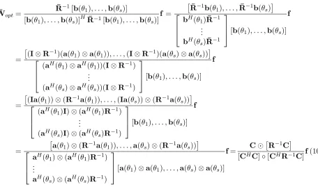
The optimal weight vector of the CME-MVDR beamformer can be obtained as follows:
¯
Wopt = R¯ −1C¯
¯
CHR¯−1C¯f (7)
It can be observed from formula (5) that the sample covariance matrix R (of N ×N order) is expanded to matrix R¯ (of N2×N2 order). From formula (6), the steering vector, a(θk) (of N ×1 order), of real antenna array is expanded to the steering vector, b(θk) (ofN2×1 order), of the SVAA through the Kronecker product operation. b(θk) can be expressed as follows:
b(θk) = a(θk)⊗a(θk) =
[
1, ej2λπdsinθk, . . . , ej
2π
λ(N−1)dsinθk
]
⊗[1, ej2λπdsinθk, . . . , ej
2π
λ(N−1)dsinθk
]
=
[
1, ej2λπdsinθk, . . . , ej2λπ(N−1)dsinθk, ej2λπdsinθk, . . . , ej2λπ(2N−2)dsinθk
]
N N - 1
real array elements virtual array elements
Figure 1. Schematic diagram of steering vector expansion of antenna array.
It can be obtained from formula (8) that there are 2N −1 non-repetitive elements in b(θk), by which virtual antenna array elements are formed. To describe it clearly, the expansion of steering vector is shown in Figure 1. It can be observed from Figure 1 that virtual array elements are formed and the real array is transformed into the SVAA.
Formula (5) can be expressed as:
¯
R=I⊗R=I⊗(UΣUH)= (I⊗U) (I⊗Σ) (I⊗U)H (9) where U denotes a matrix containing the orthonormal eigenvectors of R, and Σ denotes a diagonal matrix containing the eigenvalues ofR. The eigenvectors are corresponding to the incident directions of signals and interferences, and the eigenvalues are corresponding to the power of signals and interferences. It can be observed from formula (9) that the items I⊗U and I⊗Σ can be seen as the eigenvectors matrix and eigenvalues diagonal matrix ofR. Therefore, the information contained in¯ R¯ is the same as that inR. Besides, virtual antenna array elements are formed, so the interferences beyond the DOF of array can be suppressed by adding constraints to the SVAA beamforming method when their directions are known.
The computational load of solving formula (7) will increase with the expansion of the sample covariance matrix. The computational complexity ofR−1 isO(N3), and the computational complexity
ofR¯−1 isO(N6). However, the computational complexity of that can be greatly reduced because of the properties of an eye matrix and Kronecker product operation. According to the properties of Kronecker product operation [9], formula (7) can be simplified as follows:
¯
Wopt= R¯ −1[b(θ
1), . . . ,b(θs)]
[b(θ1), . . . ,b(θs)]HR¯−1[b(θ1), . . . ,b(θs)]
f =
[¯
R−1b(θ1), . . . ,R¯−1b(θs) ]
bH(θ1)R¯−1
.. . bH(θs)R¯−1
[b(θ1), . . . ,b(θs)]
f
=
[
(I⊗R−1)(a(θ1)⊗a(θ1)), . . . ,(I⊗R−1)(a(θs)⊗a(θs)) ]
(aH(θ1)⊗aH(θ1))(I⊗R−1)
.. .
(aH(θs)⊗aH(θs))(I⊗R−1)
[b(θ1), . . . ,b(θs)] f
=
[
(Ia(θ1))⊗(R−1a(θ1)), . . . ,(Ia(θs))⊗(R−1a(θs)) ]
(aH(θ1)I)⊗(aH(θ1)R−1)
.. . (aH(θ
s)I)⊗(aH(θs)R−1)
[b(θ1), . . . ,b(θs)] f
=
[
a(θ1)⊗(R−1a(θ1)), . . . ,a(θs)⊗(R−1a(θs)) ]
aH(θ1)⊗(aH(θ1)R−1)
.. .
aH(θs)⊗(aH(θs)R−1)
[a(θ1)⊗a(θ1), . . . ,a(θs)⊗a(θs)]
f= C⊙
[
R−1C]
[CHC]◦[CHR−1C]f(10)
where⊙denotes the KP product [11], and ◦ denotes the Hadamard product [12].
obtained by calculatingR−1 instead of calculatingR¯−1, so the computational load is greatly reduced.
The computation complexity of the optimal weight vector of the MVDR beamformer is O(N3). The
computation complexity of the optimal weight vector of the CME-MVDR beamformer isO(N3), which is equal to that of the MVDR beamformer.
4. SIMULATIONS
Assume that the narrowband excitation sources are far away from the antenna array. Consider a ULA including 4 elements, and the element space is equal to one-half wavelength. The interferences and the desired signal are all independent. The desired signal illumines on the antenna array in the direction 0◦. Two interferences whose directions are known to come from−20◦and 65◦directions. Three interferences whose directions are unknown come from −60◦, −40◦ and 25◦ directions. Signal to noise ratio (SNR) is 0 dB. Ratio of the interferences to noise is 30 dB. The number of snapshots is 200.
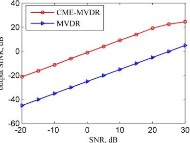
The performance of the CME-MVDR beamformer is compared with the MVDR beamformer when the two interferences with known directions are suppressed by adding constraints. Figure 2 shows the beam patterns of two beamformers. Figure 3 shows the output signal to interference plus noise radio (SINR) versus the snapshots of two beamformers. Figure 4 shows the output SINR versus the input SNR of two beamformers.
It is observed from Figure 2 that in addition to depressing the two interferences with known directions through constraints, the CME-MVDR beamformer can further depress the three interferences with unknown directions, while the MVDR beamformer is not able to suppress the three interferences with unknown directions. Thus, more interferences than the DOF of array are inhibited by the
CME-Figure 2. Beam patterns of two beamformers. Figure 3. Output SINR versus snapshots of two beamformers.
MVDR beamformer. From Figure 3, the output SINR of the CME-MVDR beamformer increases with the increase of snapshots, while the output SINR of the MVDR beamformer cannot increase with the increase of snapshots. The output SINR of the CME-MVDR beamformer is much higher than that of the MVDR beamformer. From Figure 4, the output SINR of the MVDR beamformer is very low when the number of interferences exceeds the DOF of array, because the three interferences with unknown directions cannot be suppressed by the MVDR beamformer. The output SINR of the CME-MVDR beamformer is about 20 dB higher than that of the CME-MVDR beamformer, because all the five interferences are depressed by the CME-MVDR beamformer.
As is shown in the simulation results, more interferences can be suppressed by the CME-MVDR beamformer compared with the MVDR beamformer. The performance of antenna array is improved.
5. CONCLUSION
The SVAA beamforming method based on CME is proposed, by which the real antenna array can be transformed into SVAA. More interferences than the DOF of array can be suppressed by the CME-MVDR beamformer, and higher output SINR can be obtained by the CME-MVDR beamformer compared with the MVDR beamformer. The fast calculation method of the optimal weight vector of the CME-MVDR beamformer is effective. In conclusion, the performance of antenna array beamforming is improved by the SVAA beamforming method without increasing the computational complexity.
REFERENCES
1. Zaharis, Z. D., C. Skeberis, and T. D. Xenos, “Improved antenna array adaptive beamforming with low side lobe level using a novel adaptive invasive weed optimization method,” Progress In Electromagnetics Research, Vol. 124, 137–150, 2012.
2. Huang, L., J. Zhang, X. Xu, and Z. F. Ye, “Robust adaptive beamforming with a novel interference-plus-noise covariance matrix reconstruction method,” IEEE Transactions on Signal Processing, Vol. 63, No. 7, 1643–1650, 2015.
3. Donelli, M., S. Caorsi, D. F. Natale, F. Davide, and A. Massa, “A versatile enhanced genetic algorithm for planar array design,” Journal of Electromagnetic Waves and Applications, Vol. 18, No. 11, 1533–1548, 2004.
4. Massa, A., M. Donelli, D. F. Natale, S. Caorsi, and A. Lommi, “Planar antenna array control with genetic algorithms and adaptive array theory,”IEEE Transactions on Antennas and Propagation, Vol. 52, No. 11, 2919–2924, 2004.
5. Li, W., Y.-P. Li, and W.-H. Yu, “On adaptive beamforming for coherent interference suppression via virtual antenna array,”Progress In Electromagnetics Research, Vol. 125, 165–184, 2012. 6. Blomberg, A. E. A., A. Austeng, and R. E. Hansen, “Adaptive beamforming applied to a cylindrical
sonar array using an interpolated array transformation,” IEEE Journal of Oceanic Engineering, Vol. 37, No. 1, 25–34, 2012.
7. Kim, Y.-S. and Y.-S. Kim, “Improved resolution capability via virtual expansion of array,” Electronics Letters, Vol. 35, No. 19, 1596–1597, 1999.
8. Shan, Z. L. and T. Yum, “A conjugate augmented approach to direction-of-arrival estimation,” IEEE Transactions on Signal Processing, Vol. 53, No. 11, 4104–4109, 2005.
9. Brewer, J. W., “Kronecker products and matrix calculus in system theory,”IEEE Transactions on Circuits Systems, Vol. 25, No. 9, 772–781, 1978.
10. Donelli, M. and P. Febvre, “An inexpensive reconfigurable planar array for Wi-Fi applications,” Progress In Electromagnetics Research C, Vol. 28, 71–81, 2012.
11. Liao, B. and S. C. Chan, “A cumulant-based method for direction finding in uniform linear arrays with mutual coupling,” IEEE Antennas and Wireless Propagation Letters, Vol. 13, 1717–1720, 2014.