A New Variant Of Grey Wolf Optimizer For Global Optimization

(1)

Available online: https://edupediapublications.org/journals/index.php/IJR/ Page 109

A NEW VARIANT OF GREY WOLF OPTIMIZER FOR GLOBAL

OPTIMIZATION

1

_{Amatul Ayesha Shareef,}

2

_{Dr. Syed Raziuddin,}

1

_{PG Scholar, Dept. of CSE, Deccan College of Engineering & Technology}

_Darussalam

_,

Hyderabad, Telangana, Email id: - [email protected]

2

_{Professor & HOD, Dept. of CSE, Deccan College of Engineering & Technology}

Darussalam

, Hyderabad, Telangana, Email id: [email protected]

Abstract

The Grey Wolf Optimizer is the meta-heuristics which is inspired by Grey Wolves (CanisLupis) and is

used in SI algorithms. The GWO and proposed algorithm mimics the leadership hierarchy and

hunting method of grey wolves. The four levels of grey wolves are alpha, beta, delta, and omega and

the three main steps of hunting are searching, encircling, and attacking prey. When the wolves

change from its position to attack a prey then the position has to be updated. In the GWO algorithm,

the vector location is updated by taking a simple average of best location in the pack. In proposed

algorithm the location is updated by taking an average of the weighted sum of the best locations. The

main algorithm is compared with other SI algorithm and tested over the different benchmark

functions. The dimensions of the problems are 10, 30 and 50 for comparing the proposed algorithm

over the basic state of-the-art. Simulation results support the better performance of proposed

algorithm.

Keywords: Meta-heuristic, Global Optimization, Grey Wolf Optimizer, heuristics, Swarm Intelligence.

I. INTRODUCTION

Meta-heuristics are inspired by multiple interactive agents. Agents are wolves. Metaheuristics may make few assumptions about the optimization problem being solved. Meta-heuristic optimization techniques are popular. The four reasons are

i. Inspired by very simple concepts.

ii. Flexibility refers to no changes in the structure.

iii. There is no need to calculate the derivative of search space.

iv. Avoid stagnation in local solutions and search the entire space.

So, meta-heuristics are good options for optimizing the problems.

(2)

Available online: https://edupediapublications.org/journals/index.php/IJR/ Page 110 which are used for solving the problems.

These SI algorithm mostly mimics the behavior of swarms, herds and flocks. The SI algorithm, imitates the nectar searching behavior of honeybees, egg laying and nest finding is cuckoos, light flashing of fireflies, and food searching behavior of birds is Particle Swarm Optimization. Main goal of global optimization is to find best solution to problem in presence of multiple local solutions. The GO problems are quite difficult to solve.

II. SWARM INTELLIGENCE (SI) Swarms are nothing but a group of agents of the same species. The Swarm Intelligence (SI) is define as a collective behavior of decentralized or self-organized systems. The most popular SI technique is PSO,ABC, CSA, FFA and GWO.

A. Particle Swarm Optimization (PSO): R. Eberhart and J. Kennedy said about PSO. Every individual in PSO algorithm is called as particle. The position of particle is treated to be the best possible solution. Every particle has (position, velocity, fitness). The movement of swarm is done by location update strategy which contains two best solutions: g-best is global best; p-best is personal best

B. Cuckoo Search Algorithm (CSA):

X.-S. Yang and D. Sauash said “Cuckoo Search Algorithm”. Each egg in a nest represents a solution. The cuckoo species lay the egg in the other host bird nest. The host bird on finding the egg may throw it or abandon it nest to build one. A higher quality

of egg will be carried to the next level. C. Artificial Bee Colony (ABC):

D. Karaboga and B. Bastruk said about “Artificial Bee Colony”. There are 3 types of bees: employed, onlooker and scouts. One employed bee is dedicated to one food source and their collect nectar and deposit on the hives by a waggle dance, based on the performance of the dance quality of honey is determined by onlooker bees. The employed bee becomes a scout if its food source is exhausted.

D. FireFly Algorithm (FFA):

X.-S. Yang said about firefly algorithm. Firefly algorithm is inspired by the behavior of fireflies and the motion. The main aim is mating of fireflies. The less bright firefly will be attracted towards the brighter one. A firefly is strong if its brightness is more. The 3 rules of firefly are i).Treated to be unisex i.e. firefly is attracted to other fireflies irrespective of their sex. ii). Attractiveness is inversely proportional to the distance. iii). Attractiveness and brightness are proportional to each other. E. Grey Wolf Optimizer (GWO):

(3)

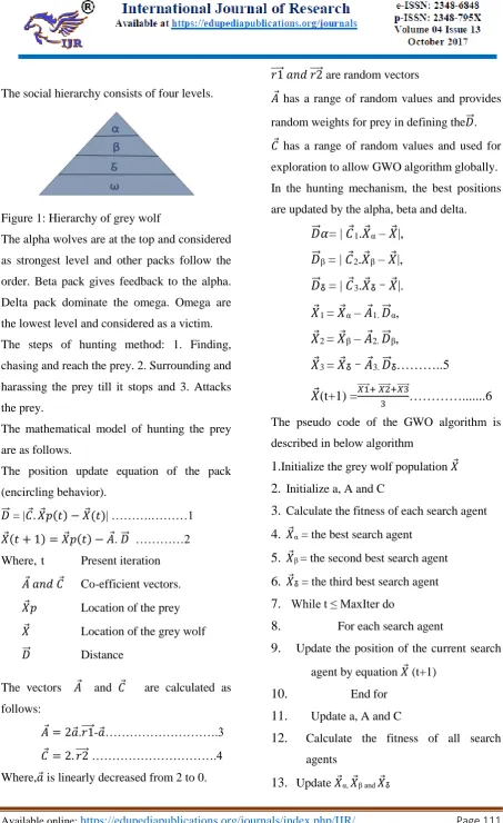
Available online: https://edupediapublications.org/journals/index.php/IJR/ Page 111 The social hierarchy consists of four levels.

Figure 1: Hierarchy of grey wolf

The alpha wolves are at the top and considered as strongest level and other packs follow the order. Beta pack gives feedback to the alpha. Delta pack dominate the omega. Omega are the lowest level and considered as a victim. The steps of hunting method: 1. Finding, chasing and reach the prey. 2. Surrounding and harassing the prey till it stops and 3. Attacks the prey.

The mathematical model of hunting the prey are as follows.

The position update equation of the pack (encircling behavior).

𝐷⃗⃗ = |𝐶 . 𝑋 𝑝(𝑡) − 𝑋 (𝑡)| ……….………1 𝑋 (𝑡 + 1) = 𝑋 𝑝(𝑡) − 𝐴 . 𝐷⃗⃗ …………2 Where, t Present iteration

𝐴 𝑎𝑛𝑑 𝐶 Co-efficient vectors. 𝑋 𝑝 Location of the prey 𝑋 Location of the grey wolf 𝐷⃗⃗ Distance

The vectors 𝐴 and 𝐶 are calculated as follows:

𝐴 = 2𝑎 .𝑟1⃗⃗⃗⃗ -𝑎 ……….3 𝐶 = 2. 𝑟2⃗⃗⃗⃗ ……….4 Where,𝑎 is linearly decreased from 2 to 0.

𝑟1

⃗⃗⃗⃗ 𝑎𝑛𝑑 𝑟2⃗⃗⃗⃗ _{are random vectors}

𝐴 has a range of random values and provides

random weights for prey in defining the𝐷⃗⃗ . 𝐶 has a range of random values and used for

exploration to allow GWO algorithm globally. In the hunting mechanism, the best positions are updated by the alpha, beta and delta.

𝐷

⃗⃗ 𝛼

= |

𝐶

1.

𝑋

α –

𝑋

|,

𝐷

⃗⃗

β = |

𝐶

2.

𝑋

β –

𝑋

|,

𝐷

⃗⃗

Ᵹ

= |

𝐶

3.

𝑋

Ᵹ

–

𝑋

|.

𝑋

1 =

𝑋

α –

𝐴

1.

𝐷

⃗⃗

α,

𝑋

2 =

𝑋

β –

𝐴

2.

𝐷

⃗⃗

β,

𝑋

3 =

𝑋

Ᵹ

–

𝐴

3.

𝐷

⃗⃗

Ᵹ

………..5

𝑋

(t+1) =

𝑋1⃗⃗⃗⃗⃗ + 𝑋2⃗⃗⃗⃗⃗ +𝑋3⃗⃗⃗⃗⃗

3

…………...6

The pseudo code of the GWO algorithm is described in below algorithm

1.Initialize the grey wolf population 𝑋

2.

Initialize a, A and C

3.

Calculate the fitness of each search agent

4.

𝑋 α = the best search agent

5.

𝑋 β = the second best search agent

6.

𝑋 Ᵹ = the third best search agent

7.

While t ≤ MaxIter do

8.

For each search agent

9.

Update the position of the current search agent by equation 𝑋 (t+1)

10.

End for

11.

Update a, A and C

12.

Calculate the fitness of all search agents

(4)

14.

t=t+1

15.

End while

16.

Return 𝑋 α

III. FRAME WORK

The search process starts in global solutions by imitating the prey hunting mechanism of grey wolves. The main criteria of proposed algorithm is the position update equation, which is taken as weighted average of the three best wolves. This result shows premature convergence and poor quality of solutions on multimodal GO problems. The position is updated by its weight in every iteration and shown in the equations. The weights wi are

calculated by taking co-efficient vectors of Ai

and Ci expressed in equation (7) and (8)

respectively. The position update strategy is calculated and by taking an average of the weights which is shown in equation (9). 𝐴 1 = 2a*𝑟 1-a, 𝐶 1 = 2. 𝑟 1…………. (7)

𝐴 2 = 2a*𝑟 2-a, 𝐶 2 = 2. 𝑟 2,

𝐴 3 = 2a*𝑟 3-a, 𝐶 3 = 2. 𝑟 3

𝐷⃗⃗ α = | 𝐶 1.𝑋 α – 𝑋 |,

𝐷⃗⃗ β = | 𝐶 2.𝑋 β – 𝑋 |,

𝐷⃗⃗ Ᵹ = | 𝐶 3.𝑋 Ᵹ–𝑋 |.

𝑋 1 = 𝑋 α – 𝐴 1 . 𝐷⃗⃗ α,

𝑋 2 = 𝑋 β – 𝐴 2 . 𝐷⃗⃗ β,

𝑋 3 = 𝑋 Ᵹ–𝐴 3 . 𝐷⃗⃗ Ᵹ.

w1=A1*C1, w2=A2*C2, w3=A3* C3………….. (8)

𝑋 (t+1) = w1X1+w2X2+w3X3

(w1+w2+w3) ……….. (9)

This pseudo code strategy is explained in below algorithm

1.Initialize iteration count (Max Iter) 2.Initialize size of the pack (NG) 3.Initialize grey wolf population X 4.Initialize a, A and C

5.Evaluate fitness of each grey wolf f(X) 6.Compute Xα=the first best grey wolf

7.Compute Xβ=the second best grey wolf

8.Compute Xδ =the third best grey wolf

9. While t <=Max Iter do 10. While i <=NG do

11. Update the position of the current grey wolf

12. End while (for i) 13. Update a, A and C 14. Update Xα, Xβ and Xδ

15. Calculate weights as per equation (8) 16. Update position vector as per equation (9) 17. Evaluate fitness of each grey wolf f(X) 18. End while

IV. EXPERIMENTAL RESULTS The coding of all the algorithms are implemented using matlab 32-bit software. The proposed algorithm is New variant GWO (NvGWO) and it is compared with other SI algorithms. The dimension of the problem is 10, 30 and 50. The proposed algorithm is working better compared to other algorithms. For every dimension the results are recorded

and presented in three ways i.e. Average,

convergence and robustness result.

AVERAGE RESULTS:

(5)

Available online: https://edupediapublications.org/journals/index.php/IJR/ Page 113 proved that the complexity of problem

increases with the dimensions. The average result of best performing algorithm is in

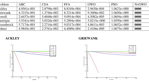
boldface. Mean results obtained by the proposed algorithm surpasses all algorithms when tested on different benchmark functions. TABLE I AVERAGE RESULTS ON 10 DIMENSIONAL PROBLEM

Problems ABC CSA FFA GWO PSO NvGWO

Ackley 4.2378e-001 3.9634e-003 5.7710e-004 3.8488e-015 1.0645e+000 0000 Griewank 4.0561e-001 2.8798e-003 8.8349e-004 5.0330e-015 1.0623e+000 0000 Powell 4.3315e-001 1.2746e-002 8.3214e-004 2.6645e-015 1.0650e+000 0000 Rastrigin 2.6437e-001 5.6048e-003 9.0914e-004 3.8488e-015 1.0694e+000 0000 Rosenbrock 3.5341e-001 3.0326e-003 5.2894e-004 2.6645e-015 1.0550e+000 0000 Sphere 5.7174e-001 2.2716e-002 9.0317e-004 4.8611e-003 1.0652e+000 0000

TABLE II AVERAGE RESULTS ON 30 DIMENSIONAL PROBLEM

Ackley 4.9845e-001 2.5761e-002 6.4089e-004 3.8488e-015 1.0645e+000 0000 Griewank 4.5594e-001 2.4285e-002 7.3452e-004 3.8488e-015 1.0623e+000 0000 Powell 2.3612e-001 3.6844e-003 4.3798e-004 5.0330e-015 1.0675e+000 0000 Rastrigin 5.6841e-001 3.3352e-002 6.1884e-004 2.6645e-015 1.0629e+000 0000 Rosenbrock 2.5605e-001 8.0000e-003 3.2952e-003 2.6645e-015 1.0638e+000 0000 Sphere 4.2378e-001 3.9634e-003 5.7710e-004 3.8488e-015 1.0645e+000 0000

TABLE III AVERAGE RESULTS ON 50 DIMENSIONAL PROBLEM

Problem ABC CSA FFA GWO PSO NvGWO

Ackley 4.0561e-001 2.8798e-003 8.8349e-004 2.9630e-004 1.0623e+000 0000 Griewank 4.3315e-001 1.2746e-002 8.3214e-004 9.3606e-002 1.0650e+000 0000 Powell 2.6437e-001 5.6048e-003 9.0914e-004 4.5082e-005 1.0694e+000 0000 Rastrigin 3.5341e-001 3.0326e-003 5.2894e-004 5.8215e+000 1.0550e+000 0000 Rosenbrock 5.7174e-001 2.2716e-002 9.0317e-004 4.8611e-003 1.0652e+000 0000 Sphere 4.9845e-001 2.5761e-002 6.4089e-004 2.4106e-009 1.0675e+000 0000

ACKLEY

0 200 400 600 800 1000 10-20

10-15 10-10 10-5 100 105

Generations

F

u

n

c

t

io

n

O

p

tim

a

A

c

h

ie

v

e

d

ABC CSA FFA GWO PSO wdGWO

Graph 1: Ackley with 10 dimension

GRIEWANK

0 200 400 600 800 1000

10-20

10-15

10-10 10-5

100

105

Generations

F

u

n

c

ti

o

n

O

p

ti

m

a

A

c

h

ie

v

e

d

ABC CSA FFA GWO PSO wdGWO

(6)

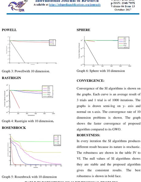
Available online: https://edupediapublications.org/journals/index.php/IJR/ Page 114 POWELL

0 200 400 600 800 1000

10-300 10-250 10-200 10-150 10-100 10-50 100 1050 Generations F u n c tio n O p ti m a A c h ie v e d ABC CSA FFA GWO PSO wdGWO

Graph 3: Powellwith 10 dimension. RASTRIGIN

0 200 400 600 800 1000 10-20 10-15 10-10 10-5 100 105 Generations F u n c ti o n O p ti m a A c h ie v e d ABC CSA FFA GWO PSO wdGWO

Graph 4: Rastrigin with 10 dimension. ROSENBROCK

0 100 200 300 400 500 600 700 800 900 1000 0 0.2 0.4 0.6 0.8 1 1.2 1.4 Generations F u n c ti o n O p ti m a A c h ie v e d ABC CSA FFA GWO PSO wdGWO

Graph 5: Rosenbrock with 10 dimension

SPHERE

0 200 400 600 800 1000 10-300 10-200 10-100 100 Generations F u n c ti o n O p ti m a A c h ie v e d ABC CSA FFA GWO PSO wdGWO

Graph 6: Sphere with 10 dimension

CONVERGENCE:

Convergence of the SI algorithms is shown on the graphs. Each curve is an average result of 3 trials and 1 trial is of 1000 iterations. The graphs is drawn semi-log on y- axis and normal on x-axis. The convergence rate of 10 dimension problems is shown. The graph shows the faster convergence of proposed algorithm compared to its GWO.

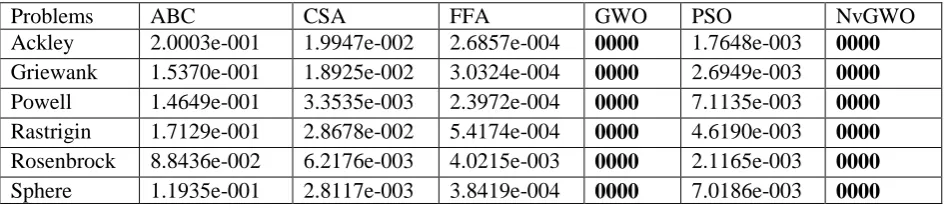
ROBUSTNESS:

In every iteration the SI algorithms produces different result because its nature is stochastic. The robustness are shown in the table IV to VI. The null values of SI algorithms shows they are stable and the proposed algorithm gives the consistent results. The best robustness is shown in bold face.

TABLE IV ROBUSTNESS ON 10 DIMENSIONAL PROBLEM

The consistency results of all the algorithm over six problems for 10 dimension shows that GWO and proposed algorithm show null value. In sphere, the proposed algorithm is performing better than GWO.

Ackley 1.1935e-001 2.8117e-003 3.8419e-004 0000 7.0186e-003

0000

(7)

Available online: https://edupediapublications.org/journals/index.php/IJR/ Page 115 Powell 2.1264e-001 1.3232e-002 6.3208e-004 0000 6.3462e-003

0000

Rastrigin 6.1893e-002 7.1871e-003 2.9242e-004 0000 4.0508e-003

0000

Rosenbrock 1.9524e-001 1.9835e-003 1.1699e-004 0000 1.5036e-002

0000

Sphere 1.1883e-001 1.9456e-002 3.4918e-004 8.4197e-003 5.4042e-003

0000

TABLE V ROBUSTNESS ON 30 DIMENSIONAL PROBLEM

The consistency results of all the algorithm over six problems for 30 dimension shows that proposed algorithm and GWO algorithm show null value.

Ackley 2.0003e-001 1.9947e-002 2.6857e-004 0000 1.7648e-003 0000 Griewank 1.5370e-001 1.8925e-002 3.0324e-004 0000 2.6949e-003 0000 Powell 1.4649e-001 3.3535e-003 2.3972e-004 0000 7.1135e-003 0000 Rastrigin 1.7129e-001 2.8678e-002 5.4174e-004 0000 4.6190e-003 0000 Rosenbrock 8.8436e-002 6.2176e-003 4.0215e-003 0000 2.1165e-003 0000 Sphere 1.1935e-001 2.8117e-003 3.8419e-004 0000 7.0186e-003 0000

TABLE VI ROBUSTNESS ON 50 DIMENSIONAL PROBLEM

The consistency results of all the algorithm over six problems for 50 dimension shows that GWO and proposed algorithm show null value except the rosenbrock function in GWO.

Problem ABC CSA FFA GWO PSO NvGWO

Ackley 1.7803e-001 3.0312e-003 2.5357e-004 0000 9.9863e-003 0000 Griewank 2.1264e-001 1.3232e-002 6.3208e-004 0000 6.3462e-003 0000 Powell 6.1893e-002 7.1871e-003 2.9242e-004 0000 4.0508e-003 0000 Rastrigin 1.9524e-001 1.9835e-003 1.1699e-004 0000 1.5036e-002 0000 Rosenbrock 1.1883e-001 1.9456e-002 3.4918e-004 8.4197e-003 5.4042e-003 0000 Sphere 2.0003e-001 1.9947e-002 2.6857e-004 0000 1.7648e-003 0000

V.CONCLUSION

The SI optimization algorithm inspired by grey wolves imitates the social hierarchy and hunting behavior of grey wolves. The wolves pack move near to attack a prey by updating position. In proposed method, update locations of the individuals in the pack by weighted average of three best locations in the pack. The performance of proposed algorithm is compared against the SI algorithms. The dimensions are 10, 30 and 50 and

comparing with the complex multi-modal benchmark problems. In simulation results shows that the proposed algorithm is better than the other SI algorithms and shows faster convergence and nature of producing better quality of solution for even higher dimensional problems and the result of the algorithm shows null deviation indicating it is stable.

REFERENCES

[1] S. Mirjajlili, S. M. Mirjajlili. A. Lewis

“Grey wolf optimizer” in 2014.

(8)

A New Variant Of Grey Wolf Optimizer For Global Optimization