Feedback Tracking and Correlation Spectroscopy of Fluorescent
Nanoparticles and Biomolecules
Thesis by
Kevin L. McHale
In Partial Fulfillment of the Requirements for the Degree of
Doctor of Philosophy
California Institute of Technology Pasadena, California
2008
Acknowledgments
Work toward this thesis began over twenty years ago when my parents, Beth and Michael, set me on the course that led to it. They will freely admit that for some time now their guidance has tended more toward the personal than the academic, but they have taught me to be the person that I am today and I can think of nothing to be more thankful for than that. I thank my sisters, Sara and Marissa, with whom growing up was always exciting and being grown up is always rewarding. Thank you to my grandmother Bernice and my extended family, in particular my cousins Michael and Linda Pisano. I also thank my newest family members, Robin, Ivy and Ian Hest. This thesis would not have been possible without all of my family’s support.
Hideo Mabuchi has been all that I could have asked for in an advisor. His patience, creativity, and confidence in the abilities of his students allows him to run a lab like no other I am aware of. The freedom afforded to me to explore my own ideas and solve problems (or to try, at least) in my own way contributed tremendously both to my learning and to my overall happiness. He has taught me how to be a scientist, and provided a model for leadership that I can only hope to emulate.
I am thankful for the guidance I have received over the years from several other scientists at Caltech. I enjoyed a rotation with Demetri Psaltis during my first year, and I appreciate and admire his willingness to spare as much time as he did. I thank my candidacy and thesis committee members, Niles Pierce, Erik Winfree, John Doyle, Changhuei Yang and Zhen-Gang Wang for their time, interest, insight and suggestions. I thank Shimon Weiss at UCLA for being a friendly link to the single-molecule community and for helping me put my work into perspective. I am also thankful to Wallace Brey, my undergraduate advisor, and Bethany Bechtel for introducing me to scientific research. Their guidance in my very early years as a scientist was an essential factor in my decision to attend graduate school.
him as a sounding board for (often far-fetched) ideas. I thank John Stocktondespitenot having written that basketball paper, and I thank Tony Miller for, well, keeping the group keen. I thank John Au for his foosball moves, Tim McGarvey for telling me about the world, Nathan Hodas for falling down a mountain with me and Luc Bouten for perpetual encouragement, friendly competition and unsolicited investment advice. Special thanks go to Sheri Stoll, my daily source of good-natured argument and the principal reason our lab ran so smoothly. Thanks also to Paul Barclay, Felipe Caycedo-Soler, André Conjusteau, Orion Crisafulli, Nicole Czakon, JM Geremia, Asa Hopkins, Joe Kerckhoff, Kenny Kwon, Ben Lev, Gopal Sarma, Andrew Silberfarb, Jen Sokol, Ramon van Handel and Jon Williams. I enjoyed working with all of you. Finally, I wish the best of luck to Charles Limouse and Michael Zhang in carrying on where I leave off.
I was fortunate to enter a Bioengineering department filled with great people. My classmates Jennifer Tom, Gwyneth Card, Jeff Endelman, Frank Lee, Derek Rinderknecht, Anna Grosberg and Princess Imoukhuede helped keep our first year fun despite certain obstacles. I shared many good times with Ben Lin, Bodhi Sansom and John Dabiri, and I will never forget the late-night trek from Ventura to Pasadena that Mike Reiser so kindly accompanied me on. I will forever be proud of founding the BEars softball team, and I am glad to leave it in the hands of Emily McDowell.
Many of my favorite times at Caltech were spent with my roommate of four years, Joe Zadeh. The story of our adventures could fill a volume at least the size of this thesis. I found great friends in Jane Khudyakov, Alexa Price-Whelan and Joe Schramm, and we had many fun times as well. I enjoyed my year playing on the Caltech rugby team and the times I shared with the team both on and off the pitch; my frequent visits to Brad Cenko’s office; dinner parties with Talia Starkey; hijinks with any combination of Will Ford, Matt Lucas and Jason Keith; dragon boat racing; foosball, Mügen, croquet and, of course, Del Taco. Most of all, I am grateful for the companionship of Megan Elizabeth Eckart, my greatest advocate and closest friend, whose support is the only thing that got me through my tumultuous final month as a grad student at Caltech.
I am fortunate to have a number of friends from home who, despite the obstacles of thou-sands of miles, three time zones and busy lives, remain close to me to this day. While keeping in touch is not always easy, it is a true testament to my friendships with David Abramson, Samantha Martin, Steve Kay, Phillip Crandall and Mike Flamino that while our lives are always changing, things between us always seem to stay the same. All of you are on my mind more than you know.
Abstract
The best way to study dynamic fluctuations in single molecules or nanoparticles is to look at only one particle at a time, and to look for as long as possible. Brownian motion makes this difficult, as molecules move along random trajectories that carry them out of any fixed field of view. We developed an instrument that tracks the Brownian motion of single fluorescent molecules in three dimensions and in real-time while measuring fluorescence with nanosecond time resolution and single-photon sensitivity. The apparatus increases observation times by approximately three orders of magnitude while improving data-collecting efficiency by locking tracked objects to a high-intensity region of the excitation laser.
As a first application of our technique, we tracked and studied the fluorescence statistics of semiconductor quantum dots. Our measurements were well resolved at 10ns correlation times, allowing measurement of photon anti-bunching on single particles in solution for the first time. We observed variations of (34±16)% in the fluorescence lifetimes and (23±18)% in the absorption cross-sections within an aqueous quantum dot sample, confirming that these variations are real, not artifacts of the immobilization methods previously used to study them. Additionally, we studied quantum dot fluorescence intermittency and its dependence on 2-mercaptoethanol, finding evidence that the chemical suppresses blinking on short time-scales (<1s) by reducing the lifetime of the dark state.
Contents
Acknowledgments iii
Abstract v
Contents vi
List of Tables xi
List of Figures xii
1 Introduction 1
1.1 Personal history . . . 3
1.2 Experimental history . . . 5
1.3 Organization of the thesis . . . 6
1.4 Publications resulting from graduate work . . . 8
2 Three-dimensional localization of a fluorescent particle 9 2.1 Beam symmetry and DC symmetry breaking . . . 9
2.2 Particle localization in two dimensions via spatial beam modulation . . . 12
2.2.1 Position-dependent fluorescence rate modulation . . . 13
2.2.2 Lock-in detection: demodulation of AC signals . . . 13
2.2.3 The two-dimensional localization signal . . . 15
2.2.4 Two-dimensional localization noise . . . 17
2.3 Three-dimensional localization . . . 19
2.3.1 More on beam geometry . . . 20
2.3.2 Localization signal for the symmetric geometry . . . 22
2.3.3 Localization signal for the asymmetric geometry . . . 23
2.3.4 Radial localization with three-dimensional modulation . . . 25
3 Tracking system dynamics 28
3.1 The feedback loop . . . 28
3.1.1 Brownian motion . . . 30
3.1.2 Localization noise process . . . 33
3.1.3 Controller and plant dynamics . . . 34
3.1.4 Localization estimate . . . 34
3.2 Linearized tracking dynamics . . . 35
3.2.1 Input-output statistics . . . 35
3.2.1.1 The caseu(t)=N(t) . . . 36
3.2.1.2 The caseu(t)=xp(t) . . . 36
3.2.2 Second-order dynamics . . . 37
3.2.2.1 Tracking error statistics . . . 38
3.2.2.2 Stage position increment statistics . . . 39
3.3 Nonlinear limitations in real tracking systems . . . 41
3.3.1 Bandwidth-limited steady-state error . . . 42
3.3.2 Escape time statistics . . . 44
4 Fluorescence correlation spectroscopy 49 4.1 Open-loop FCS . . . 50
4.1.1 The correlation functiong2(τ) . . . 50
4.1.2 Single-component FCS . . . 52
4.1.3 Incorporating additional dynamics . . . 54
4.1.4 The effect of background counts . . . 55
4.2 Tracking-FCS . . . 56
4.2.1 General calculation of the tracking-FCS curve . . . 57
4.2.1.1 Example: solid particle in a stationary Gaussian beam . . . 61
4.2.1.2 Example: free particles in a harmonic potential . . . 61
4.2.2 General properties of tracking-FCS curves . . . 62
4.2.3 Dynamic light scattering and other related techniques . . . 64
4.2.4 Contributions due to modulated beams . . . 66
5 Experimental apparatus and diagnostic results 70 5.1 Design overview . . . 70
5.1.1 Modulation optics . . . 70
5.1.2 Additional optics, detectors and feedback electronics . . . 74
5.1.3 Probe beam . . . 75
5.2.1 Lasers . . . 76
5.2.2 Modulators . . . 77
5.2.3 Optics . . . 80
5.2.4 Mechanical components . . . 82
5.2.5 Acquisition hardware and software . . . 84
5.2.6 Control Electronics . . . 85
5.2.6.1 Modulation electronics . . . 85
5.2.6.2 Post-detection electronics . . . 86
5.3 Experimental procedures . . . 92
5.3.1 Bead immobilization . . . 92
5.3.2 Beam scans . . . 93
5.3.3 Localization signal measurement . . . 94
5.3.4 Alignment . . . 94
5.3.5 Tracking system characterization . . . 96
5.3.6 Delay calibration . . . 97
6 Photon statistics of quantum dot fluorescence 99 6.1 Introduction . . . 99
6.1.1 Quantum dots . . . 99
6.1.2 Photon statistics . . . 101
6.1.3 Motivation for our work . . . 102
6.2 Photon statistics of a two-level emitter . . . 103
6.2.1 Evolution of the Master equation . . . 104
6.2.2 Computing waiting-time statistics . . . 105
6.2.3 Effect of background counts . . . 107
6.2.4 Effect of additional emitters . . . 108
6.2.5 Implications of the Cauchy-Schwarz inequality: photons! . . . 108
6.3 Experimental measurements of quantum dot anti-bunching . . . 110
6.3.1 Data . . . 111
6.3.2 Recovery rate heterogeneity . . . 114
6.3.3 Evidence of multiple excitations . . . 117
6.3.4 Absolute detection efficiency calibration . . . 119
6.4 Blinking statistics . . . 122
6.4.1 Three-state model . . . 122
7 Structural fluctuations in isolated DNA molecules 130
7.1 Theoretical dynamics of linear polymers . . . 132
7.1.1 Static properties of flexible polymers . . . 132
7.1.2 Generalized dynamics of polymer solutions . . . 134
7.1.3 Harmonically-bound submolecules: the Rouse model . . . 136
7.1.4 Hydrodynamic interactions: the Zimm model . . . 139
7.1.5 Chain stiffness: semiflexible chain . . . 140
7.2 Fluorescence correlation spectroscopy of polymers . . . 141
7.2.1 Dynamic structure factor . . . 142
7.2.2 Application to open-loop FCS . . . 145
7.2.3 Tracking-FCS of polymers . . . 146
7.3 Literature review . . . 148
7.3.1 Lumma et al.,Phys. Rev. Lett., 2003 . . . 148
7.3.2 Shusterman et al.,Phys. Rev. Lett., 2004 and Petrov, et al.,Phys. Rev. Lett., 2006 . . . 149
7.3.3 Cohen and Moerner,Phys. Rev. Lett., 2007 . . . 149
7.4 Measurements . . . 151
7.4.1 Center of mass motion . . . 154
7.4.2 Internal motion . . . 155
8 Concluding remarks 159 A Signal analysis via recursive Bayes estimation 160 A.1 Introduction . . . 160
A.2 Derivation of probability distributions . . . 162
A.2.1 Recursive Bayesian estimator . . . 163
A.2.2 Effective diffusion statistics . . . 164
A.2.3 Fluorescence photon detection statistics . . . 165
A.2.4 Practical Considerations . . . 166
A.2.5 Experimental regimes . . . 167
A.2.6 Generalizing the approach . . . 168
A.3 Simulations . . . 170
A.3.1 Identification based on diffusion coefficient . . . 171
A.3.2 Multiple species identification . . . 175
A.3.3 Slow-diffusion identification . . . 177
A.3.4 Background noise and estimator performance . . . 180
A.5 Perturbative calculation ofp(nk=0|rk;rk−1;ξk;sj) . . . 181
B Statistical limits to dilute concentration estimation 183 B.1 Introduction . . . 183
B.2 Statistics of exact particle detection . . . 185
B.2.1 Detection-region diffusive influx dynamics . . . 187
B.2.2 Particle-detection statistics . . . 188
B.3 Concentration estimation . . . 189
B.3.1 Universal limit to estimator performance . . . 189
B.3.2 Near-optimal time-domain concentration estimator . . . 191
B.3.3 Time-domain variance and concentration fluctuations . . . 192
B.4 Experimental considerations . . . 193
B.4.1 Localization inaccuracy . . . 193
B.4.2 Recurrent detections . . . 194
B.4.3 Entry-time determination methods . . . 195
B.4.4 Bias due to multiple occupancy . . . 196
B.5 Simulations . . . 198
B.5.1 Concentration estimation with exact particle detection . . . 198
B.5.2 Concentration estimation via fluorescence detection . . . 200
B.5.3 Estimation of dynamic fluctuations in mean concentration . . . 202
B.5.4 Simultaneous multiple-species concentration estimation . . . 203
B.6 Discussion . . . 207
List of Tables
2.1 Parameters for axial localization signal plots. . . 23
6.1 Parameters for exponential fits. . . 127
6.2 Parameters for stretched-exponential fits. . . 129
List of Figures
1.1 Example single-molecule fluorescence experiment. . . 2
1.2 Example single-molecule fluorescence signal. . . 3
2.1 Contour plot of a diffraction-limited 532nm Gaussian beam. . . 10
2.2 Beam rotation and fluorescence intensity modulation. . . 12
2.3 Two-dimensional localization signals for different rotation geometries. . . 16
2.4 Optical modulation for three-dimensional localization. . . 19
2.5 Three-dimensional geometries for modulated beams. . . 21
2.6 Axial localization signals. . . 24
3.1 Tracking system feedback loop. . . 29
3.2 Tracking error simulation with different feedback bandwidths. . . 30
3.3 Brownian motion. . . 32
3.4 MSD(∆t)with varied system parameters. . . 40
3.5 Steady-state tracking error due to nonlinearity. . . 43
3.6 Steady-state occupancy of the linear region. . . 44
3.7 Splitting probabilityπ0 a(e0). . . 45
3.8 Choosingε. . . 46
3.9 Mean escape time. . . 47
4.1 Example open-loop fluorescence data and FCS curve. . . 51
4.2 Example single-component FCS curves. . . 55
4.3 Example tracking-FCS curves. . . 63
4.4 Tracking-FCS curves with 3-D modulated laser beams. . . 68
5.1 Acousto-optic modulator. . . 71
5.2 Focusing of laser beams. . . 72
5.3 Photo of modulation optics and beam paths. . . 73
5.4 Schematic of the apparatus. . . 74
5.6 Filter layout. . . 81
5.7 Assembled microscope stage. . . 82
5.8 Coverslide holder. . . 83
5.9 Photo of control electronics. . . 86
5.10 Modulation electronics schematic. . . 87
5.11 Detection electronics schematic. . . 88
5.12 532nm and 415nm beam comparison. . . 93
5.13 Localization error signals. . . 95
5.14 24nm bead tracking. . . 96
5.15 Tracking-FCS curve for 24nm fluorescent beads. . . 97
5.16 Delay calibration. . . 98
6.1 Two-level emitter energy level diagram. . . 100
6.2 Anti-bunching correlation function with finite pulse width. . . 111
6.3 Qdot tracking data. . . 112
6.4 Anti-bunching rise rate vs. excitation intensity. . . 113
6.5 Standard deviation of anti-bunching recovery rates. . . 114
6.6 Likelihood function for standard deviations of fit parameters. . . 116
6.7 Anti-bunching attenuation factor. . . 117
6.8 Simple multiple-electron qdot model. . . 119
6.9 Photon collection from a single qdot. . . 120
6.10 Averaged qdot fluorescence intensity. . . 121
6.11 Simple three-state blinking model. . . 123
6.12 Average tracking trajectory durations at eachC2ME, with 2σ error bars. . . 125
6.13 Tracking-FCS of blinking Qdots. . . 126
6.14 Fits to blinking FCS data. . . 127
6.15 Fits to blinking FCS data. . . 128
7.1 Illustration of a labeled DNA molecule. . . 131
7.2 Freely-jointed polymer model. . . 133
7.3 Rouse/Zimm model. . . 136
7.4 Exact and approximate Rouse DSF. . . 145
7.5 Example tracking data. . . 152
7.6 Averaged mean-squared deviation curve for tracking stage data. . . 153
7.7 Example tracking-FCS curves. . . 155
7.8 Variation in measuredg2(τ)curves with label density of 1 dye : 150bp. . . 156
A.1 Data generated by two-dimensional simulation. . . 170
A.2 Simulated photon counts. . . 171
A.3 Sample spatial distributions. . . 172
A.4 Spatial estimator performance with varied diffusion coefficient ratios. . . 173
A.5 Identification performance with varied diffusion coefficient ratios. . . 174
A.6 Identification performance with multiple sample components. . . 175
A.7 Identification performance with multiple sample components. . . 176
A.8 Comparison of estimator performance using binned and exact data. . . 177
A.9 Exact estimator performance with varied background levels. . . 179
A.10 Binned estimator performance with varied background levels. . . 179
B.1 Concentration fluctuations at different concentrations. . . 185
B.2 Illustration of the sample regions described in the text. . . 186
B.3 Time-scale separation of first detection and recurrent detection. . . 195
B.4 Bias and variance of the corrected estimator at varied concentrations. . . 197
B.5 Concentration estimation for free, unbiased diffusion. . . 199
B.6 Concentration estimation within a micro-channel. . . 200
B.7 Example fluorescence trace. . . 202
B.8 Concentration estimates derived from fluorescence data. . . 203
B.9 Dynamic estimation of fluctuating concentrations. . . 204
Chapter 1
Introduction
We are only beginning to understand the degree to which biology is influenced by consequences of the size of its basic building blocks. Nucleic acids and proteins are special in that they are big, but not too big, relative to the size of the water molecules that surround them. Under constant bombardment by surrounding fluid, biological molecules bend, stretch, vibrate, fold and unfold, break apart and recombine; these dynamics almost certainly influence the way in which they interact with each other. Small molecules do not behave like this because the stiffness of their chemical bonds prevents such structural fluctuations; nor do large objects, because viscous drag quickly dampens any acceleration due to small collisional forces. These types of motions are uniquely the domain of large molecules, most often biological molecules, and their exact characteristics and the extent of their consequences are still widely unknown.
Dynamic fluctuations in the shapes of molecules are hard to detect because no two molecules experience the same sequence of collisions, so no two molecules exhibit the same fluctuations. Any attempt to study such fluctuations among large numbers of molecules will fail, because the motion of each molecule is drowned out by the motion of all the others. For most of the history of science, we have therefore been limited to the measurement of the average, equilibrium properties of microscopic biological systems.
Pinhole Detector Dichroic
Mirror
Microscope Objective
Excitation
Figure 1.1: Example single-molecule fluorescence experiment. The pinhole reduces background from out-of-focus fluorescence emitters.
focused by a high power microscope objective to a small, intense spot within a liquid sample. Fluorescent molecules — or molecules labeled by a fluorescent probe — drift into and out of the beam as they move by Brownian motion, the translational motion due to collisions with solvent molecules. The fluorescence emitted by the molecules is collected by the objective and focused onto a sensitive detector. The resulting signal is either a high time-resolution sequence of fluorescence bursts, like that illustrated in Fig. 1.2, or a lower time-resolution but spatially resolved image of the molecule and its surroundings.
Single-molecule fluorescence measurements have some limitations that are apparent just from the appearance of the data in Fig. 1.2. The duration of each burst is determined by the molecule’s motion, and typically limited to less than 10ms (longer for imaging methods, but still limited). This places restrictions on the time-scales that can be probed using these methods. Many biological molecules have interesting dynamics that are on time-scales as long as or longer than this, and therefore that cannot be resolved by these measurements. In addition, we only collect a finite number of photons from each molecule, and this number determines how well the molecule’s dynamics can be resolved: the fewer pairs of photons are detected with time-spacing ∆t, the larger the measurement uncertainty becomes on that time-scale. This fundamental type of noise arises any time a process is described by a continuous rate but mediated by discrete events[8, e.g.]. We could try to reduce this noise by increasing the intensity of the excitation laser, but dye saturation and bleaching will always limit our ability to do this.
0 5 10 15 20 25 30 0
50 100 150 200 250 300 350 400
Time [ms]
F
luor
esc
enc
e (10
3
phot
ons / s)
Figure 1.2: Example single-molecule fluorescence signal. Molecules emit bursts as they drift through the focus of the excitation laser.
is to understand biology then we should be concerned about the influence of the attachment surface on the molecule stuck to it. At the very least we expect it to perturb the molecule’s structure by concentrating at the point of attachment all of the forces incident on the molecule due to solvent collisions. The chemistry of the attachment surface can influence the molecule as well: glass surfaces, for example, often carry an electrical charge that will affect the molecule through electrostatic forces.
Over the last few years, several groups[9–15] have begun to develop a new technology for extending single-molecule observation times using feedback control. These approaches allow the molecule to move freely in solution while active hardware moves some combination of the microscope optics or sample stage in order to keep the molecule in focus at all times. These techniques in principle would allow for the completely passive observation of individual molecules often for times that are orders of magnitude longer than they would be in the absence of feedback. This thesis documents my work, primarily over the past 18 months, in developing what is arguably the most capable of these techniques yet developed.
1.1
Personal history
I would do once I arrived.
I knew when I committed to Caltech that I would be a part of a very young Bioengineering program, but I failed to fully anticipate the extent to which this would affect me. Fortunately I had a good group of friends in my classmates, and by supporting each other we made it through the rough times and — I hope — helped improve the program for those that succeeded us.
I began doing research in my second term, when I worked with Demetri Psaltis on a project comparing the imaging properties of insect-inspired compound lens systems with more tradi-tional simple lens systems. My goal in this project was to determine applications for which a synthetic version of such an imaging system might be particularly useful. Over the course of the term I — with the help of insightful discussions with Michael Dickinson at Caltech and Simon Laughlin at the University of Cambridge — came to the conclusion that compound eyes did not evolve for their imaging properties, and that a compound lens system would likely only be favored in applications in which imaging performance was not the primary design parame-ter. Demetri’s guidance on this project kept me excited about doing research, and the project itself sparked an early interest in optics that would develop through the remainder of my time in grad school.
I attribute my meeting of Hideo Mabuchi to serendipity alone. In my first term at Caltech I registered for a course in control theory, a subject I had never previously studied. One com-ponent of that course was a weekly guest lecture on applications of control theory in Caltech labs. I did not attend those lectures regularly, but happened to attend one that Hideo gave about laser stabilization, Michael Armen’s adaptive homodyne experiment and the early stages of John Stockton’s magnetometry experiment. I thought it was interesting, and a few months later I found myself emailing Hideo about doing a research rotation in his lab.
Hideo answered my email almost immediately, we met, and he suggested I talk to Andrew Berglund about some of the recursive estimation algorithms he had been working on for his FRET microscopy experiment. I began working with Andy on a statistical method for identifying molecules based on individual fluorescence bursts in single-molecule experiments, and over the course of that term I wrote code to simulate fluorescence data and implement the identification algorithm. I officially joined Hideo’s lab over the summer, and we submitted a paper on my work in December 2003[16].
discussions with Hideo, Andy and Igor Mezic at UCSB about the relationship between mixing and reaction statistics in extremely dilute solutions. This work, combined with some comments from a referee of my first paper, motivated me to write a paper about the effects of counting noise on estimates of the concentration of dilute solutions.
While working on concentration estimation, I took a bit of a detour to work with John Au on his application of convex optimization techniques to the design of photonic bandgap crystal structures. I had studied convex optimization during my first year at Caltech, and I was glad to be able to revisit the subject with a real application to work on. For a few months, John and I worked in parallel: he developed the physical theory and I wrote optimization software that was custom-tailored to his problem. In the end my code became a fairly robust interior-point solver, we both learned a lot about optimization, and John went on to develop an iterative method for designing photonic crystal structures with optical properties that are potentially useful for atomic physics experiments.
I finished my candidacy exam in November 2005, proposing to apply my identification and concentration estimation algorithms to problems in molecular biophysics. Almost immediately afterward, I began working on something very different and never turned back. As an apology to my candidacy committee, this was truly not my intention — I distinctly remember a conver-sation with Megan Eckart about the fluorescence microscopy experiment in which she asked why we needed so many optics and I replied that those were for the tracking apparatus, and that I “had no interest” in that. Andy and I began working together under the premise that he would teach me to use his microscope so that I could work on my proposed experiments while he was working on the tracking apparatus. Literally within hours we had taken the entire apparatus apart, and so began my work on particle tracking.
1.2
Experimental history
I began working on the apparatus with Andy in late 2005 and we quickly realized that it needed to be rebuilt as a dedicated tracking microscope in order to optimize its performance. Over the next 6 months, through improvements of the mechanical and electronic components, beam and detector alignment, background noise rejection, beam intensity control and general experimental technique, we developed an apparatus that was capable of tracking 60nm and 210nm fluorescent nanospheres in two dimensions with accuracy limited almost entirely by photon-counting noise (with a signal size of about 4500 photons/sec)[19]. With our experiments complete, Andy began writing his thesis while I set out to completely rebuild the apparatus once again.
I began constructing an apparatus for tracking single fluorescent particles in three dimen-sions during the summer of 2006, basing it on Hideo’s ideas for using a pair of laser beams to track particles along the optic axis of the microscope. That apparatus began operating in November 2006, and with it I demonstrated tracking of individual semiconductor quantum dots freely-diffusing in water[20]. I was able to resolve fluorescence anti-bunching on single quantum dots in solution, allowing me to characterize heterogeneity in quantum dot fluorescence statis-tics as well as fluorescence intermittency on time-scales as long as 1s. These measurements highlighted the importance of tracking techniques for making new types of measurements on single fluorescent objects, and also represented a technological advance in that no comparable technique had yet tracked objects that moved this quickly.
More recently, I have focused on tracking single DNA molecules for the evaluation of theo-retical predictions for the internal Brownian dynamics of polymers in solution. While several measurements of this type have been made over the past few years[21–25], it is my view that none combines sufficient theoretical rigor with experimental data that can provide conclusive arguments for or against particular predictions. This is the motivation for my work in this area.
1.3
Organization of the thesis
I have made an effort to make this thesis entirely self-contained, which applies primarily to its theoretical components. In the first two chapters, this means including detailed reviews of relevant work in particle-tracking experiments before introducing my own work that is ei-ther specifically relevant to tracking in three dimensions or just an aspect of particle tracking dynamics that I find interesting. The last two chapters deal with applications of the tracking apparatus that themselves require a bit of theory, and those theories are reviewed with a level of detail dictated by the applications.
begins with a review of the theory behind two-dimensional localization, most of which was developed by Andy Berglund. The chapter continues by extending the discussion to three-dimensional localization, in which I derive the basic properties of the localization method that we developed.
Chapter 3 reviews the dynamics of the tracking system. I discuss the feedback loop that the tracking system is based on, and review the linearized theory developed by Andy Berglund for describing the statistics of the tracking system in a “good” tracking limit. I conclude the chapter by deriving some of consequences of position estimation nonlinearity on the tracking statistics — in particular, I find nearly exact expressions for the statistics of particle escape from a tracking system by using a first-passage time approach.
Chapter 4 begins with a basic review of Fluorescence Correlation Spectroscopy (FCS)[1, 26], a single-molecule technique that we apply to our measured fluorescence signals. Next, I derive in a very general way the statistics of FCS for a tracked particle with internal degrees of transla-tional freedom in preparation for the study of the intramolecular dynamics of DNA molecules.
Chapter 5 describes the experimental apparatus in detail.
Chapter 6 discusses the application of the tracking apparatus to the study of semiconduc-tor quantum dots. The chapter begins with a background discussion on quantum dots, and develops a theoretical model for describing the basic properties of their fluorescence statistics. Next I present my measurements of photon anti-bunching in freely-diffusing quantum dots, and a detailed analysis of those measurements. I conclude with a basic theoretical description of quantum dot blinking statistics, and present our measurements in this area.
Chapter 7 describes the application of the apparatus to the study of the dynamics of the motion ofλ-phage DNA. This chapter begins with a detailed discussion of the basic polymer dynamics theories that are necessary for understanding some of the arguments, mostly against the validity of certain approaches taken in the literature, later in the chapter. It concludes with a set of measurements on both the translational and intramolecular dynamics of the DNA molecules. This work remains ongoing.
Chapter 8 is a brief conclusion and discussion.
statistics of the waiting times between single-molecule detections, and evaluate its performance on simulated data and in comparison to alternative methods. It will be published eventually, but likely in a less-detailed form.
1.4
Publications resulting from graduate work
While at Caltech my work resulted, at least in part, in several publications that have either appeared in peer-reviewed journals or are almost ready to be submitted.
1. K. McHale, A. J. Berglund and H. Mabuchi. “Bayesian estimation for species identification in single-molecule fluorescence spectroscopy.” Biophys. J.86, 3409 (2004).
2. K. McHale, A. J. Berglund and H. Mabuchi. “Near-optimal dilute concentration estimation via single-molecule detection.” In preparation.
3. J. K. Au, K. McHale and H. Mabuchi. “Inverse problem based design of photonic crystal devices — Part II.”In preparation.
4. A. J. Berglund, K. McHale and H. Mabuchi. “Feedback localization of fluorescent particles near the optical shot-noise limit.” Opt. Lett.32, 145 (2007).
5. A. J. Berglund, K. McHale and H. Mabuchi. “Fluctuations in closed-loop fluorescent particle tracking.” Opt. Express15, 7752 (2007).
6. K. McHale, A. J. Berglund and H. Mabuchi. “Quantum dot photon statistics measured by three-dimensional particle tracking.” Nano Lett. 7, 3535 (2007).
Chapter 2
Three-dimensional localization of a
fluorescent particle
Both the most difficult and the most important task in closed-loop particle tracking is the esti-mation of the position of the particle being tracked. Tracking errors must be sensed accurately and quickly in order for the feedback system to correct them before the particle escapes. Any noise intrinsic to the localization method will limit its accuracy; any latency in the localiza-tion estimate will limit the tracking bandwidth. Furthermore, the sensitivity of the localizalocaliza-tion method will often determine the amount of time for which particles can be tracked: the more photons are needed for localization, the faster the tracked particle bleaches and the sooner it becomes invisible to the apparatus.
We begin this chapter with a discussion of the symmetry-breaking requirements necessary for measuring three-dimensional position estimates for a single fluorescent particle, and we discuss several methods that involve symmetry-breaking in the fluorescence detector. We next introduce temporal symmetry breaking using spatial beam modulation, discussing the method used by several groups, including ours, for two-dimensional localization and tracking. Finally, we present the method that we have developed for three-dimensional localization and conclude with a derivation of the localization noise statistics intrinsic to this method.
2.1
Beam symmetry and DC symmetry breaking
Traditional single-molecule fluorescence microscopes, such as that depicted in Fig. 1.1, employ non-imaging detectors that do not provide enough information to determine the positions of detected particles because both the excitation laser beam and the collection and detection optics are highly symmetric. A focused TEM00 Gaussian laser beam has the intensity profile[27]
I(x, y, z)= 2P
π w2(z)exp
"
−2x 2+y2
w2(z)
#
x [µm]
z [
µ
m]
−1 −0.8 −0.6 −0.4 −0.2 0 0.2 0.4 0.6 0.8 1 −1
−0.8 −0.6 −0.4 −0.2 0 0.2 0.4 0.6 0.8 1
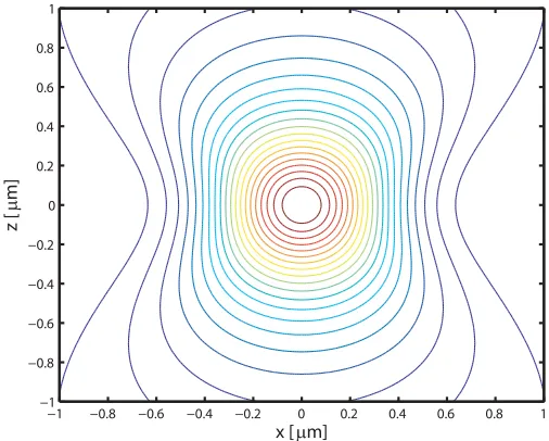
Figure 2.1: Contour plot of a diffraction-limited 532nm Gaussian beam.
wherePis the total optical power in the beam,zis the axis of beam propagation, thez−dependent waist is given by
w2(z)=w2 0
1+ zλ π w2
0
!2
, (2.2)
and we have allowed the beam centroid to lie at the coordinate origin. We sometimes define the Rayleigh rangezR =π w02/λfor notational simplicity in later sections. Figure 2.1 shows a cross-section of this profile for a beam withλ=532nm that is focused to its diffraction limit (w0 = λ/2). The consequences of the beam symmetry, as it relates to tracking, are obvious from the contour plot: because the only measurement available to us is the fluorescence rate, we cannot distinguish between any points that lie on the same contour surface. In order to track, something must be done to break this symmetry.
Symmetry-breaking approaches tend to fall into two categories: either the symmetry of the beam is broken while the detection optics are unchanged, or vice-versa. Outside of our group, most methods rely on breaking symmetry in the detection optics using imaging detectors, such as quadrant photodiodes or charge-coupled device (CCD) cameras. These detectors have good two-dimensional spatial resolution (along the x and y axes) and have been used for localization in several closed-loop particle tracking experiments[13–15, 28–31]. However, no optical detector technologies offer three-dimensional position sensitivity, so additional work is necessary to localize particles in three dimensions.
image, and the relationship between the sizes of the ellipse axes is determined by the particle’s displacement from the focal plane of the laser beam[32]. A CCD records images of the fluores-cence, and computer software computes position estimates in real time based on the shape of the fluorescence ellipse. A second method tracks the particle along thex andy axes using a quadrant detector and locks the particle’szposition in a plane either above or below thexy
plane. The combination of the laser beam’s divergence and the decaying detection efficiency along thezaxis induced by the use of a confocal pinhole creates a steep enough intensity gra-dient to estimate the particle’s position directly from the detected fluorescence intensity: if the intensity is too high (low), the tracking system should move the particle further from (closer to) the beam centroid[15, 31]. These approaches have been used to track fluorescent particles in viscous solutions, with diffusion coefficients as high as 0.6µm2/s, roughly corresponding to a 700nm diameter sphere in water.
The localization techniques described in this section all encode position information in low-frequency components of the fluorescence — either as the size of the differential signal between pixels in an imaging detector or simply as the absolute fluorescence intensity. Such position estimates are subject to systematic low-frequency noise sources that limit their track-ing fidelity. The sensitive photodetectors necessary for detecttrack-ing strack-ingle molecules will always detect a background signal from scattering and auto-fluorescence in the glass coverslides, am-bient scattered laser light, room lighting in the laboratory, power LEDs on equipment, etc. Any fluctuations in the size of these background signals — due to, for example, spatially nonuni-form impurities in coverslides or 60Hz noise from AC power lines — feed into the position estimates and cause tracking errors. Even more importantly, any internal dynamics of the particles being tracked — blinking of dyes or quantum dots, or conformational motion of a polymer, for example — also couple into the localization estimates. Imaging methods tend to be less sensitive to these types of noise than intensity-based methods because they are bal-anced: such noise is correlated across all pixels on the detector, but only differential signals appear in the position estimates. This may explain why two-dimensional tracking methods us-ing imagus-ing detectors have greatly outperformed three-dimensional methods that incorporate intensity-basedzlocalization[30, 31]. However, no detector is perfectly balanced and even the detectors themselves, in the absence of incident light, produce low-frequency noise that can have a significant impact on the localization signals. For more information on the ubiquity of low-frequency noise, see [33, 34].
2.2.1
Position-dependent fluorescence rate modulation
As illustrated in Fig. 2.2, we let xs(t)be the position of the tracking stage and xp(t)be the position of the tracked particle at timet. For a Gaussian laser beam, the fluorescence intensity depends only on the relative coordinatee(t)=xp(t)−xs(t). If the beam is rotating at frequency
ωxy with rotation radius r, and we define the focused waist w(0) = w0, we calculate the fluorescence intensity from Eq. 2.1:
Γ(e, t)=χI(e, t)=Γ0exp
(
− 2
w02 h
(ex(t)−rcosωxyt)2+(ey(t)−rsinωxyt)2
i )
, (2.3)
where χ is the fluorescence scattering coefficient of the particle and Γ0 = 2P χ/π w02 is the fluorescence intensity of a particle located at the origin. We can express this simply in polar coordinates as
Γ(e, t)=Γ0exp
(
− 2
w02 h
ρ2+r2−2r ρcos(ωxyt−φ)
i )
, (2.4)
where, as usual,ρ≡ kekandφ≡tan−1[e y/ex].
Equation 2.4 gives us the quantitative form of the intuitive fluorescence rate modulation that we described earlier and illustrated in Figure 2.2. The size of the oscillating term in the exponent is proportional toρ, andφis exactly the phase angle of the oscillation. Before we try to make quantitative sense out of it, however, we first discuss the very general problem of demodulation of AC signals. This topic deserves its own sub-section because it is very important to the functioning of our apparatus.
2.2.2
Lock-in detection: demodulation of AC signals
In the previous section we derived Eq. 2.4, which we know contains information describing the two-dimensional positionxp in the magnitude and phase of itsωxy oscillation. The question now is how to extract that information efficiently. Here we solve the general problem, where our signal consists of a superposition ofN sinusoidal terms at distinct frequencies and we must measure the magnitude and phase of one of them. This procedure is referred to as
phase-sensitiveorlock-indetection, and is exactly how laboratory lock-in amplifiers work. Specifically, ifu(t)is a signal that can be written as a finite sum of sine waves,
u(t)= N
X
n=0
ancos(ωnt−φn) , (2.5)
completely free of systematic noise (although laser intensity noise appears in theajterm, as we will discuss in the next section). Furthermore, we may encode additional information — such as the zposition of the particle for three-dimensional tracking — at other high frequencies, and there will be hardly any cross-talk between the demodulated signals if those frequencies are sufficiently separated fromωxy.
2.2.3
The two-dimensional localization signal
Before actually calculating what the localization signal is, we should consider what we want it to be. The output of our lock-in amplifiers will consist of a separate analog electronic signal for each Cartesian axis. Those signals should equal zero when the particle is on the axis of the beam rotation, and should vary linearly with the particle’s distance from the origin so that it is easy to translate the electronic signals to real position estimates. Of course, this linearity must break down at some point, because we cannot localize the particle when it is far from the rotation axis since it will be only very weakly illuminated by the laser beam.
The fluorescence signal collected by our detector consists of a stream of photons
ξ(t)= N
X
j
δ(t−tj), (2.9)
where the arrival timestj are random variables drawn from a point process[8] with modulated rate given in Eq. 2.4 andδ is the Dirac delta function. Each photon produces an electronic pulse h(t) on the output of the detector that is then used for localization measurements. The complete electronic signalu(t)is the convolution ofξ(t)andh(t), but for simplicity we assume thath(t) is itself a sharply-peaked function that integrates toV0. This way, on time-scales relevant to our localization estimate (time-time-scales comparable to or longer than ω−1
xy),
h(t)≈V0δ(t)and we have
u(t)≈V0ξ(t). (2.10)
We use lock-in detection to extract the magnitude and phase of the ωxy component of
u(t); due to the stochastic nature of the detected fluorescence signal, this output is a random process. We must characterize this random process by computing its expected value, which will tell us the average value of the position estimate for a particle at positione. For this we must use the statistics of rate-modulated Poisson processes[8, 37]: ifξ(t)is the derivative of a Poisson counting process (as defined in Eq. 2.9) and the rate of this process isΓ(t), then
hξ(t)i =Γ(t) (2.11)
rotating at frequencyωxyare focused at different depths inside the sample, separated by about 1µm, and the total excitation power is alternated between the beams at frequencyωz. As in two-dimensional localization, the particle’s position in thexyplane is encoded in the magnitude and phase of theωxyfrequency component of the fluorescence signal. The particle’s position inzis encoded in the signal in a similar way: as shown in the plot in Fig. 2.4, theωzfrequency component of the fluorescence signal is either in-phase or 180◦out-of-phase with theω
zdrive signal, depending on whether the particle is above or belowz=0. The magnitude of theωz component is proportional to the particle’s distance to the origin. Optical power modulation can easily be done at high frequencies: we typically useωz =2π×100kHz, with a demodulation bandwidthB∼1kHz. This bandwidth will almost never be the limiting factor in single-particle tracking applications, because photon-counting noise will typically place a much lower limit on the localization bandwidth.
Using a pair of beams in three dimensions introduces several free parameters describing the beam geometry that are not present in two dimensions: each beam is focused in a different plane, with a different minimum waist. In addition to the waist of the beam, the rotation radius
r also depends on z, forming a cone that focuses down so thatr (z0)=0 at some depth z0. Before characterizing the localization statistics of this method quantitatively, we will describe the beam geometry in further detail.
2.3.1
More on beam geometry
To generally describe the two localization beams we must keep track of thez-dependent waist and rotation radius of both beams separately, but this would produce extremely complicated mathematical descriptions that, in practical terms, are unnecessary. Instead, we will assume that the focused waists w0 of the two beams are identical and that the angle of divergence of the cone of rotation is identical for the two beams. They are then allowed to differ only in whether the beam waist focuses to its minimum above or below the rotation cone. In practice, it should be possible to create a pair of beams that are very close to identical, so this assumption is not overly restrictive.
z = 0 2z0
z1
Beam 1 Beam 2
z = 0 2z0 z
1 Beam 1
Beam 2
a)
b)
−10 0 10 −0.4
−0.2 0 0.2 0.4
−10 0 10 −0.4
−0.2 0 0.2 0.4
−10 0 10 −0.4
−0.2 0 0.2 0.4
−10 0 10 −0.4
−0.2 0 0.2 0.4
e
z[
µ
m]
−10 0 10 −0.4
−0.2 0 0.2 0.4
e
z[
µ
m]
−10 0 10 −0.4
−0.2 0 0.2 0.4
e
z[
µ
m]
e
ze
za)
b)
c)
d)
e)
f )
Chapter 3
Tracking system dynamics
In the last chapter we discussed the optical method that we use to compute estimates of a fluorescent particle’s position. This discussion focused entirely on static properties of the localization system; we did not consider the fact that the particle is moving and the tracking stage is following it. This chapter takes a very general result from the previous chapter — the fact that we have a well-characterized, accurate method to estimate the position of a fluorescent particle — and builds a feedback loop around it. We account for the dynamics of the particle’s motion and the statistical properties of the localization estimate, showing how they affect the statistics of the tracking stage. In particular, we concern ourselves with the statistics of tracking errors — the deviations between the stage and particle positions. When these errors are small relative to the laser beam rotation radius, we are able to characterize them analytically in almost exact detail. When the errors are not so small — typically due to a particle that moves too fast for the feedback system to keep up — the localization estimates lose fidelity and the resultant tracking statistics are much more complicated. The chapter concludes with a discussion of some of the consequences of these larger errors and strategies that may be used to avoid them.
3.1
The feedback loop
N(t)
Noise
x
s(t)
e(t)
x
p(t)
e(t)
P(s)
C(s)
Localization
Estimate
Figure 3.1: Tracking system feedback loop. The tracking errore(t)— the difference between the particle’s positionxp(t)and stage positionxs(t)— causes fluorescence rate modulation that is used to estimatee(t). The error estimate ˆe(t)is fed into the feedback controller (with transfer functionC(s)), and this drives the tracking stages (which have transfer functionP (s)) in order to cancel the tracking error.
we feature it as an additive inputN(t)to ˆeso that we can compute its effects on the tracking system dynamics later in this chapter.
Once ˆehas been constructed it is fed into a feedback controller, denoted by theC(s)block in the diagram. The output of this controller is fed into the “plant” P (s), consisting of the combination of the tracking stages and the electronic amplifiers that drive them. The stage positions feed back subtractively intoe, hence closing the loop.
The feedback loop is designed to drive ˆeto zero; since ˆeis an unbiased estimate ofe, this implies that e is, on average, zero as well. However, since ˆe is related to e by the addition of noise, enforcing ˆe(t) = 0 corresponds toe(t) = N(t), so that the localization noise feeds directly into tracking errors. Of course, all tracking systems have finite bandwidth so it is not possible to achieve ˆe(t) = 0; as a result, both the localization noise and the motion of the particle contribute to the tracking error.
0 0.2 0.4 0.6 0.8 1 −2
0 2 4 6
Position [
µ
m]
0 0.2 0.4 0.6 0.8 1
−4 −2 0 2 4
Time [s]
Residual [
µ
m]
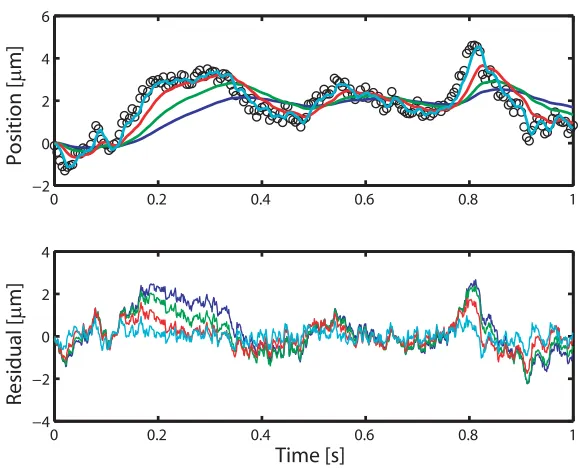
Figure 3.2: Top: Simulation of a diffusing particle (black circles) with diffusion coefficient
D=10µm2/s. We compute the trajectories of the tracking stage that are exact up to a random value for the initial state of the stage. The parameters describing the tracking system are defined in later sections; we used a second-order system with γp = 100Hz and controller bandwidthγc = 1Hz (blue), 2Hz (green), 5Hz (red) and 20Hz (cyan). Bottom: tracking error
e=xp−xs.
3.1.1
Brownian motion
Before we go on to characterize the tracking system, we must have an adequate description of its inputs and constituent blocks. We begin withxp, following the Langevin derivation of the Brownian motion. For more information about this approach, see [8, 39, 40]. An excellent historical discussion of Brownian motion can be found in [40].
As discussed in Chapter 1, the particle’s motion is caused by collisions between it and the molecules in the solvent surrounding it. All of the solvent molecules are in constant motion due to their thermal energy. Each time one of these molecules collides with the particle, the particle experiences a very small impulsive force pushing it in the direction the molecule was moving in. The thermal motion is uncorrelated between different solvent molecules, so that each collision pushes the particle in a different direction. We assume that the liquid molecules are very small relative to the particle, and that the mean free path between the molecules and the particle is very small. Therefore, the particle experiences a very large number of collisions in any short period of time.
system is chosen, the particle’s motion all three axes may be treated independently; there is no correlation between motion along orthogonal axes. As a result, henceforth we deal only with the scalarxp representing any of the three components ofxp.
The force exerted on the particle alongxp is a rapidly-fluctuating function that we denote
B(t). We write the particle’s equation of motion as
mp d2
dt2xp= −γ d
dtxp+B(t), (3.1)
wherempis the mass of the particle and theγ term represents the Stokes drag on the particle due to the viscosity of the solution. We must specify B(t) in order to make any sense out of Eq. 3.1. The only tractable description ofB(t)is as a stochastic process — anything else would require that we keep track of the dynamics of all of the molecules in the solvent — so we characterizeB(t)by its statistical properties. First,hB(t)i =0 because we assume that there is no convective drift in the particle’s position. Second, we letB(t)be delta-correlated because each collision is very short:
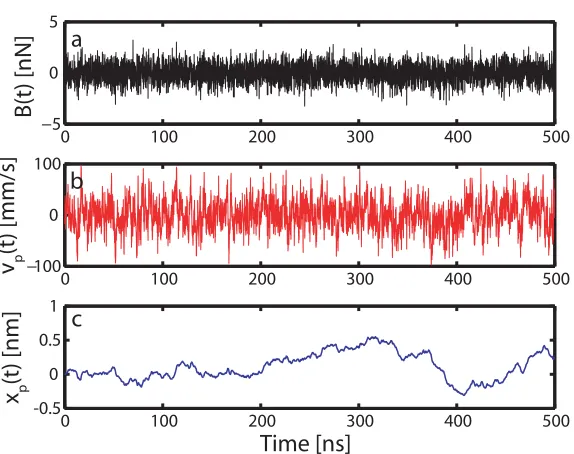
hB(t1)B(t2)i =Υδ(t2−t1), (3.2) whereΥ is a constant that we will determine by physical arguments once we solve Eq. 3.1. This correlation time of zero characterizesB(t)aswhite noise, because it implies (via the Wiener-Khinchin theorem) thatB(t)has a constant power spectral density. Finally, we assume that the distribution ofB(t)is Gaussian with zero mean and varianceΥ. Figure 3.3aillustrates a real-ization of the processB(t)simulated according to this description, with physical parameters chosen to correspond to a polystyrene sphere in water.
We may integrate Eq. 3.1 easily because it is linear, and we do so to get
vp(t)≡ d
dtxp =e
−γt/mpv
p(0)+ 1
mp
e−γt/mp Zt
0
dτ eγτ/mpB(τ), (3.3)
where we defined the velocityvp for notational convenience. Figure 3.3bshows the particle’s velocity computed from the simulated B(t). Using Eq. 3.3, we may compute the mean and correlation function of the velocity:
hvp(t)i =e−γt/mpvp(0) (3.4) hhvp(t1)vp(t2)ii =
Υ 2γmp
h
e−γ|t1−t2|/mp−e−γ(t1+t2)/mpi, (3.5)
steady-0 100 200 300 400 500 −5
0 5
B(t) [nN]
0 100 200 300 400 500
−100 0 100
v
p(t) [mm/s]
0 100 200 300 400 500
-0.5 0 0.5
1
x
p(t) [nm]
Time [ns]
a
b
c
Figure 3.3: Simulated Brownian motion of a 1µm polystyrene sphere in water. We simulated the random force B(t)(a, top) and computed the resulting particle velocityvp(t)(b, middle) and position xp(t) (c, bottom). Simulation parameters: r = 0.5µm, η = 10−3 Pa·s (water),
ρp =1.005g/cm3(polystyrene),T =298K.
state energy of the particle is exponential, with meankBT wherekB is Boltzmann’s constant andT is the temperature of the liquid. It is simple to show that this implies thatvp, related to the energy byE=mpvp2/2, obeys
lim t→∞hvp(t)
2i =kBT
mp
. (3.6)
We use this to determine the size of the fluctuations inB(t)from Eq. 3.5:
Υ =2kBT γ. (3.7)
Due to our assumption thatB(t)is Gaussian, the higher cumulants ofvp all vanish. In other words,vp is itself Gaussian, so that it is fully characterized by its mean and variance.
We may simplify Eqs. 3.4 and 3.5 considerably if we are only interested in times much longer than the correlation timeτc = mp/γ. The Stokes drag coefficient for a spherical particle of radiusr is given byγ =6π r η, whereηis the viscosity of the solvent[41]. This implies that
result, the long-time approximation
hvp(t)i =0
hvp(t1)vp(t2)i =2Dδ(t2−t1),
(3.8)
where D = kBT /γ is the particle’s diffusion coefficient, is always sufficient to describe the dynamics we observe in this thesis.
Given the random processvp, all that remains is the integration
xp(t)=
Zt
0
dτ vp(t) (3.9)
from which we compute the statistical properties ofxp. Using Eq. 3.8, we get
hxp(t)i =0 (3.10)
hxp(t1)xp(t2)i =2Dmin{t1, t2}, (3.11)
which illustrates an important characteristic of the mean-squared displacement: it scales in proportion tot for Brownian motion, while it usually scales ast2for objects that move deter-ministically.
3.1.2
Localization noise process
The second input to the feedback loop is the localization noiseN(t). Arising due to photon-counting noise as described in Section 2.2.4,N(t)is a zero-mean random process with variance determined by the beam geometry, averaging bandwidthB, electronic gainV0AV and photon counting rateΓ. Because the correlation time of the photon-counting fluctuations is very short (see Eq. 2.12), the correlation time ofN(t)is set by the averaging as approximatelyB−1. Bis typically much larger than the tracking bandwidth, soB−1is much shorter than the time-scales of the motion of the tracking stages. Therefore we may approximate the statistics
hN(t)i =0 (3.12)
hN(t1)N(t2)Ti ≈n2Idδ(t1−t2), (3.13)
3.1.3
Controller and plant dynamics
We assume that both the controller and the plant respond linearly to their inputs. While this may seem restrictive, most control electronics and many stage actuators — in particular, our piezoelectric actuators — are very nearly linear. Given this assumption, the inputs (generically denotedu(t)) and outputs (y(t)) of both blocks satisfy a dynamical system of the form
d
dtq(t)=Aq(t)+Bu(t) y(t)=Cq(t),
(3.14)
whereqis an internal state vector and the matricesA,BandCare together referred to as the
state-space representation of the system. An alternative representation of the system that is often useful is found by taking the Laplace transform of Eq. 3.14, giving
˜
y(s)=C(sId−A)−1Bu(s).˜ (3.15)
The quotient ˜y(s)/u(s)˜ is known as thetransfer functionfromutoy. The notationsC(s)and
P (s)from Fig. 3.1 represent the transfer functions of the controller and plant, respectively. Their combined transfer function is simply the productC(s)P (s)which, if not for the presence of the localization block, would be referred to as theloop transfer functionbecause it maps the input to the output of the feedback loop.
3.1.4
Localization estimate
We let the localization estimation block be composed of a single functionL[e]that mapseinto hˆei. Then
ˆ
e(t)=L[e]+N(t). (3.16)
Special consideration must be given to the two casesu(t) = N(t)and u(t) = xp(t) due to fundamental differences arising from the forms of their correlation functions (Eqs. 3.11 and 3.13). In particular, N(t) is a delta-correlated stationary process andxp(t) is not, and this difference has a major effect on the statistics of the output signals.
3.2.1.1 The caseu(t)=N(t)
SinceN(t)is delta-correlated, the integrals in Eq. 3.20 collapse into the single integral
hhyN(t1)yN(t2)ii =n2C
Zmin{t1,t2} 0
dτ eA(t1−τ)BBTeAT(t2−τ)CT, (3.21)
where the subscript notation is used to keep track of the input signal. The explicit dependence of this expression on t1 andt2 is a consequence of our derivation of it by solving an initial value problem. This is clear from the fact thathy(0)i =Cq0andhhy(0)2ii =0. This transient artifact is eliminated by settingt2=t1+τ and taking the limitt1→ ∞. The resulting integral
Σ∞≡ lim t1→∞
Zt1 0 d
τ eA(t1−τ)BBTeA(t1−τ) (3.22)
converges when the eigenvalues ofAare all negative, which is a prerequisite for stability of the feedback system[43]. We are left with the simple expression
yN(t+τ)yN(t)=n2CeAτΣ∞CT. (3.23)
3.2.1.2 The caseu(t)=xp(t)
Things get complicated whenu(t)=xp(t)becausexpis not delta-correlated. Neither integral in Eq. 3.20 disappears, and the minimum function in Eq. 3.11 requires us to divide the inte-gration region into three parts based on the relationship betweent1 andt2 in each part. The integral does not converge ast→ ∞, making matters even worse.
The calculation is simplified somewhat if we consider the transfer function from vp(t), rather thanxp(t), toy(t). The integral relatingvp(t)toxp(t)gives us
˜
y(s)
˜
vp(s) = 1
s
˜
y(s)
˜
xp(s)
, (3.24)
which says that usingvp(t)as our input to the system produces precisely the time derivative ˙
order system parameters. All curves shareMSD(0)=0 because the tracking stage moves with a finite bandwidth andMSD(∞)=Dbecause the dynamics of the tracking stage become iden-tical to those of the particle at long times. The rise time and overshoot, and more specifically the functional form ofMSD(∆t)on intermediate time-scales, are consequences of the system parameters. Plotashows that the rise times decrease with increasing loop gain but that there is significant overshoot whenγcis too large due to the phase lag in the plant dynamics. The curve atγc = 71Hz represents the optimal value for this parameter. Plotbshows that local-ization noise can have a dramatic effect on the stage dynamics at short time-scales, but must be suppressed on longer time-scales because otherwise the tracking system would not follow the particle. Plotcshows that the effect ofN(t)onMSD(∆t)depends in part onD: it is more noticeable whenDis small compared ton.
3.3
Nonlinear limitations in real tracking systems
The previous section illustrated the importance of the simplification of the tracking system dynamics resulting from setting L[e] = e. We were able to fully characterize the statistics of all relevant variables in the feedback loop. In doing this we showed the existence of a bandwidth-limited tracking regime (see Eq. 3.32) in which our localization statistics cannot be improved by adjusting the gain in the feedback loop and depend on the diffusion coefficientD. This means that for any real tracking system with finite actuation bandwidthγp, the linearity approximation is guaranteed to fail for sufficiently small particles (with sufficiently largeD). In this section, we consider this fundamental limit to tracking system performance.
The standard deviation of the tracking error under the linear approximation (with optimal
γc) is given by Eq. 3.32. As shown in Section 2.2.3, the linear localization region in two
dimen-sions is the disk bounded by the rotation radiusr, related to the beam waistw0byw0≈r √
2. This allows us to calculate the diffusion coefficient threshold for remaining within the linear regime with 95% probability:
D.n2γp2+w 2 0γp
8 −
nγ2 p 2
v u u t4n2+
w02 γp
. (3.36)
WhenDis greater than the threshold in Eq. 3.36, the tracked particle spends some of its time at the fringes of the localization signal. The linearity approximation breaks down, making it very difficult to analytically compute statistics such asστ
α andMSD(∆t). In fact, sinceL[e] decays to zero for largeethe particle will, with probability 1, eventually escape the tracking apparatus so that our entire model of the tracking system breaks down. We take an approach in this section that is meant to characterize this phenomenon — to determine some simple statistics of escape.
Throughout the remainder of this section we setn=0 — this just means that we are capable of collecting enough photons from the particle so that localization noise does not limit our tracking fidelity. Our concern is therefore strictly with tracking inaccuracy due to the particle’s movement, although it is just a generalization of our approach here to incorporate localization noise into our model. For a complete discussion of localization noise-limited tracking see [36, 37].
3.3.1
Bandwidth-limited steady-state error
We may evaluate just how the nonlinear position estimate affects the tracking statistics by considering the steady-state distribution of the particle relative to tracking stage. For simplicity, we will approximateP (s)=1, so that the tracking system has first-order dynamics. While this model does not actually exhibit bandwidth-limited feedback because takingγc→ ∞(withn=0) reduces the tracking error to zero, any finiteγcyields the tracking errorσα0=
p
D/γc and the diffusion coefficient thresholdD.w02γc/8.
We may write a stochastic differential equation for the error:
d
dte(t)=vp(t)−γcL[e(t)]. (3.37)
This nonlinear equation is difficult to solve exactly, but it can be shown that it is equivalent to the Fokker-Planck equation for the probability density functionp(e, t)[8],
∂
∂tp=γc ∂
∂e L[e]p
+D ∂
2
∂e2p, (3.38)
10−1 100 101 102 0.1
0.2 0.3 0.4 0.5 0.6 0.7 0.8 0.9 1 1.1
γ
c/D [
μ
m
-2]
P(|e|<r)
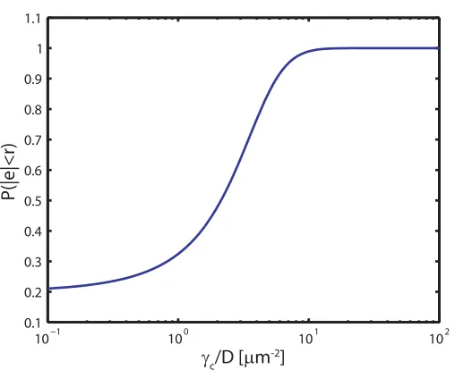
Figure 3.6: Steady-state occupancy of the linear region. We computed Eq. 3.40 at varied values of γc/D and integrated the stationary distribution over the linear region |e| < r. We fixed
w0=r √
2 in these calculations.
abrupt transition suggests that there is not much room for a “nonlinear tracking” regime — the particle is apparently either tracked well, with a stationary distribution that closely resembles the predictions of the linearized theory, or it is not tracked at all. We consider this idea more thoroughly in the next section.
3.3.2
Escape time statistics
As shown in the last section, the effect of the nonlinearity inL[e]on the steady-state distri-bution of the tracking error is fairly dramatic. There is a sharp transition from apparently not tracking at all to tracking perfectly over an order of magnitude increase in the tracking band-width. However, it is not obvious how to interpret this in a dynamic context; a given steady-state distribution tells us nothing about the rate at which the particle transitions from being tracked to not being tracked. Such dynamic properties are most appropriately studied using the statis-tics of first passage t