Urban groundwater extraction in Kuala Lumpur, Malaysia

(1)

Kuala Lumpur, Malaysia

Master Thesis

Civil Engineering & Management July 4th_{, 2008}

Author: Pieter E. Stek

(2)

Summary

The purpose of this study is to evaluate the feasibility of groundwater extraction in Kuala Lumpur, Malaysia as a potential source of potable water. Kuala Lumpur’s current water supply is provided by large reservoirs that are dependent on rainfall. In 1998 a long period of drought caused a severe water shortage, demonstrating the vulnerability of these reservoirs.

Since that time, the city’s water supply infrastructure has been expanded in line with its fast-growing economy and population. In the Ninth Malaysia Plan, an important policy document, the Malaysian government stated its intention to further expand Kuala Lumpur’s water supply, including from alternative sources such as groundwater, to meet growing water demand (EPU, 2005).

This makes a study on the feasibility of groundwater extraction in Kuala Lumpur very timely. Three aspects of groundwater extraction are evaluated: technical feasibility, economic feasibility and institutional feasibility. Together, they provide a comprehensive picture.

Technical feasibility is evaluated by constructing a groundwater flow model capable of predicting the physical effects of groundwater extraction. The model uses borehole data (groundwater depth), remote sensing data (elevation, evaporation) and water balance data (rainfall, hydrological measurements, leakage from water pipes). Because of Kuala Lumpur’s complex geology some model parameters, such as hydraulic conductivity, cannot be measured directly and must be calibrated.

The model results suggest that two extraction strategies are feasible: small scale permanent extraction (2.5% of water demand) or large scale temporary extraction (25% of water demand). The weakness of the model results lies in the underlying model assumptions that cannot be verified with the available data.

Accepting the model results at face value, an economic comparison with the Selangor Pahang Water Transfer Scheme suggests the costs of groundwater extraction are competitive, especially for a large scale temporary extraction. Nevertheless, uncertainty remains over the potential cost of necessary environmental remediation and how groundwater extraction costs compare to alternatives, such as programs to reduce non-revenue water.

The institutional feasibility of groundwater extraction is hindered by a lack of knowledge and the large number of agencies that have unclear responsibilities and jurisdictions with respect to groundwater resources management. Furthermore, Kuala Lumpur’s water utility is loss-making and the state governments, who carry a constitutional responsibility for water supply and water resources management, have a weak financial position relative to the federal government (Jomo, et al., 2003).

(3)

The study does not allow a definitive conclusion about the feasibility of groundwater extraction in Kuala Lumpur to be drawn, but the positive results do suggest that further research should be conducted to explore the full potential of the city’s urban groundwater resources.

(4)

Introduction

1.1

Background and Research Scope

Kuala Lumpur is a major economic centre in Southeast Asia (Figure 1) with a rapidly growing population and economy. This growth has been accompanied by a rapid expansion of the city’s infrastructure, including its water supply infrastructure. Kuala Lumpur relies almost exclusively on rain-fed reservoirs which make its water supply susceptible to disruptions when there is inadequate rainfall. A serious three-month water shortage in 1998 demonstrated the vulnerability of the city’s reservoirs.

To prevent a recurrence of the 1998 drought and to expand the city’s water supply, the Malaysian federal government announced in the Ninth Malaysia Plan (2006-2010), its most important policy document, that “... development of groundwater will be promoted as interim [an] measure[s] to address the anticipated shortage of water in Selangor, Kuala Lumpur and Putrajaya” (EPU, 2005).

Figure 1 – Map of West Malaysia. Labeled are Selangor state and the federal territories of Kuala Lumpur and Putrajaya.

Groundwater is often seen as a reliable source of clean water that is available close to the point of consumption, making it an ideal source for meeting the demand for potable water in urban areas. But in urban areas in particular, aquifers are often threatened by pollution and over-extraction which can destroy these groundwater resources.

(6)

quality, environment, land-use, economy and even governance and social concerns (World Bank, 2000; Custodio, 2002).

Although necessary, sustainable groundwater management is complex and it requires extensive technical knowledge (World Bank, 2000). Unfortunately in many cases even elementary

groundwater data such as hydraulic conductivity and recharge cannot be obtained through direct measurements or it is prohibitively expensive to do so (Lerner, 2002; Lubczynski, et al., 2005). Therefore groundwater models play an important role in estimating parameters, organising data and studying the dynamics and sensitivity of the groundwater system (Anderson, et al., 1992).

The lack of reliable data causes uncertainty. Uncertainty, along with the problem’s complexity, the long-term time-scale of groundwater changes and pluralism (i.e. the presence of multiple policy actors) can prevent effective decision-making, especially if there is a lack of incentives to explore win-win situations or profitable trade-offs between policy actors (Bressers, et al., 2003). In Kuala Lumpur the lack of knowledge about groundwater has been highlighted in several water resource studies, but no comprehensive groundwater monitoring and modelling efforts have been undertaken as yet to reduce this knowledge deficit (Binnie dan Rakan, 1980; LESTARI, 1997; SMHB, 2000; Madsen, et al., 2003; Hamsawi, 2007). At present groundwater is not used as a source of potable water for Kuala Lumpur. Large surface water reservoirs are used instead to capture and store the necessary water and their capacity continues to be expanded (Hamsawi, 2007; LESTARI, 1997).

Nevertheless, there are a growing number of incentives that make groundwater an attractive potential source of potable water for Kuala Lumpur. Besides the growth in water demand due to an expanding population and economy and the threat from pollution to lakes and rivers, Kuala Lumpur’s rain-fed reservoirs are sensitive to prolonged periods of drought which led to a serious water shortage in 1998 (EPU, 2005; JAS, 2007; Hamirdin, et al., 2004). A recurrence of a water shortage like the one in 1998 is possible given the tight balance between water supply and demand and the effects of climate change (Hamirdin, et al., 2004).

Hence it is timely to re-evaluate the potential of Kuala Lumpur’s groundwater resources as a source of potable water. In doing so, attention should be given to two clear deficits in current knowledge. Firstly, the technical feasibility of groundwater extraction must be addressed. Secondly, it should become clear why, given the prevalence of several incentives mentioned in the previous paragraph, no comprehensive studies of groundwater resources have yet been undertaken in Kuala Lumpur and no comprehensive groundwater management policy has been formulated.

1.2

Objectives and Research Questions

(7)

Hence, the objective of this study is: to evaluate the feasibility of urban groundwater extraction in Kuala Lumpur as a source of potable water.

Feasibility is usually assumed to consist of three factors: technical feasibility, economic feasibility and institutional feasibility. These three factors are congruent with the knowledge deficits mentioned earlier: hydrogeology (technical feasibility) and governance (economic and institutional feasibility). Economic considerations are regarded as the primary incentives for cooperation and decision-making by policy actors and are therefore an important governance issue.

These considerations lead to the formulation of three research questions related to the objective stated above:

1. What are the physical effects of groundwater extraction? 2. What is the economic value of groundwater extraction?

3. What is the current institutional setting with respect to groundwater resource management and how can it be changed to enable groundwater extraction?

1.3

Outline

(8)

2

Quantification of Groundwater Resources

2.1

Introduction

The quantification of groundwater resources often proves to be a formidable challenge. It is difficult to quantify groundwater resources because required data acquisition can be prohibitively expensive. Just like the exploitation of oil and gas reserves, exploration costs account for a large part of the investment needed to safely exploit groundwater resources. Hence it is important to quantify groundwater resources accurately and cheaply early on in the development process so that the necessary information is available for timely decision-making. There are several different methods of groundwater quantification, one of them is modelling. Groundwater models can be used to study the sensitivity and dynamics of the groundwater system and to organize available field data (Anderson, et al., 1992). This gives modelling a significant advantage when analysing Kuala Lumpur’s very inhomogeneous hydrogeology over other quantification methods such as pumping tests and groundwater potential mapping. Pumping testsa_{are primarily influenced by local hydrogeological conditions and therefore, if the} hydrogeology is highly variable, the results are not valid for a wider area and therefore of limited value in larger-scale groundwater studies (Lubczynski, et al., 2005). Groundwater potential mappingb_{is a very powerful tool for estimating groundwater recharge in large} vegetated areas. However in urban areas recharge is heavily influenced by factors such as leaking pipes and complex land use for which groundwater potential mapping methods are ill-suited (Lerner, 2002).

The purpose of the groundwater flow model described in this chapter is to answer the first research question: What are the physical effects of groundwater extraction? By predicting the effects of groundwater extraction using the model, different extraction strategies can be compared.

In this chapter the theory of modelling and the selection of an appropriate model are addressed first (Section 2.2). After this, the available data is analysed and processed so that it can be used as an input for the model (Section 2.3). Next are the setup and calibration of the model (Section 2.4), followed by the evaluation of several different extraction strategies to provide an answer to the research question (Section 2.5).

2.2

Modelling Theory and Model Selection

In this section the relevant literature about groundwater and groundwater modelling is

reviewed as it pertains to Kuala Lumpur. This leads to the selection of a modelling method (the Equivalent Porous Medium method) and a model (MODFLOW). Both the theory and equations behind the model and the modelling method are described. Lastly, the concept of dual-porosity

a_{Pumping Test: a method for determining the transmissivity (hydraulic conductivity x aquifer thickness) and}

storativity (volume of water released from storage per unit decline in the hydraulic head) of an aquifer and to establish the reliable yield of a well and to find out if the well affects other wells and springs.

b_{Groundwater Potential Mapping: a method for estimating groundwater recharge using climate (e.g. rainfall,}

(9)

media is mentioned. Although the concept is not applied in the modelling process, it does offer some valuable insights.

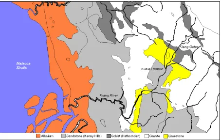
The hydrogeology of Kuala Lumpur is complex. Granite, Hawthornden (mostly schist), Kenny Hills (mostly sandstone) and Kuala Lumpur Limestone formations are overlaid by fluvial deposits (. The latter three formations: Kenny Hills, Kuala Lumpur Limestone and the fluvial deposits have groundwater potential, and thus a relatively high hydraulic conductivity and storage (LESTARI, 1997; Yin, 1986; Freeze, et al., 1979).

Figure 2 – Geological map of the Klang basin, including Kuala Lumpur.

Hydraulic conductivity, K (m/day), is the main determinant of groundwater flow velocity and a core parameter in any groundwater model. The relationship of hydraulic conductivity to flow, q (m/day) and the hydraulic gradient, Δh/Δx (m/m) is expressed by Darcy’s fluid permeability equation (1). It assumes laminar flow through a porous medium and is given for a single dimension, x.

(1)

The groundwater flow equation (4) is the basis of any groundwater flow model. It is derived from Darcy’s equation (1) and the mass balance equation (2). The groundwater flow equation is valid for a representative elementary volume: a theoretical volume that is large enough to have a representative porosity, small enough to have a near-constant hydraulic head and through which there is again laminar flow (Anderson, et al., 1992).

(10)

(2)

The mass balance equation (2) can be rewritten into a flux balance equation (3) because water is assumed to be incompressible. Since mass = density × volume and density is constant, density can be left out of the equation. Since we are considering the 1-dimensional situation, volume = Δx.

The storativity coefficient, S (m/m), is introduced on the left-hand-side of the equation to express the storage properties of the aquifer. Storativity expresses the volume of water that is released from an aquifer per unit decline in the hydraulic head. In an unconfined aquifer, storativity is assumed to be equal to specific yield (i.e. drainable porosity) because the elastic storage (water released when aquifer is still fully saturated) is very small relative to the

drainable porosity. Typical values of specific yield are: 14% (limestone), 26% (schist), 21% (fine sandstone) and 6% (clay) (Anderson, et al., 1992).

(3)

By replacing the in- and out-going flux in equation (3) with the Darcy equation we can derive the 1-dimensional groundwater equation (4) which can be re-written as the analytical

3-dimensional groundwater equation (5) that is used in groundwater flow models. Note that qsource and qsink have been combined into R (m/day), a generic source/sink term that can also be used to express leakage. Also note that volume (now 3D: x, y, z) and storativity are moved to the right-hand side of the equation and that hydraulic conductivity and storativity are considered to be spatially uniform and isotropic within the representative elementary volume (Anderson, et al., 1992).

(4)

(5)

Although the groundwater flow equation is very elegant and widely used, the assumptions on which it is based, such as uniformity and laminar flow, cannot always be satisfied in practise. The fluvial deposits and the Kuala Lumpur Limestone formation violate the model assumptions. The limestone formations contain many fractures, conduits and cavities created by chemical erosion of the carbonate. This creates a two-phase system of nearly impermeable carbonate rock and conduits with rapid, non-laminar flows (Yin, 1986; Anderson, et al., 1992). In the fluvial deposits, the transmissivity can vary by 2 to 3 orders of magnitude due to the grain size distribution, making it difficult to measure or to define the boundaries of a representative elementary volume (Freeze, et al., 1979; Lubczynski, et al., 2005).

(11)

In that case the non-laminar flow through fractures, conduits and cavities is assumed to

‘average out’. If spatial and temporal groundwater head data is available, then parameters such as hydraulic conductivity can be calibrated (Scanlon, et al., 2003).

To apply the Equivalent Porous Medium method, a numerical model is needed that compliments the structure of the data. The data is available in fixed grids (see next section) therefore a finite difference model seems appropriate which also uses fixed grids. The most popular finite difference model is the Modular Finite-Difference Groundwater Flow model (MODFLOW), developed by the United States Geological Survey. ‘Modular’ refers to the fact that different modules, such as a recharge module, river module, wells module, etc. can be added to the model when they are needed, making the model very flexible. Most previous Equivalent Porous

Medium studies use MODFLOW (Quinn, et al., 2006; Scanlon, et al., 2003).

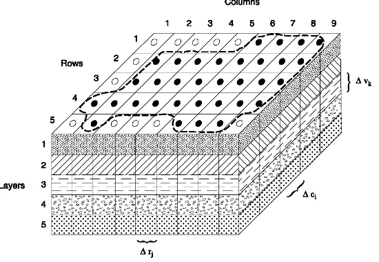
Given below is a schematisation of MODFLOW (Figure 3) and the analytical equation that is solved in MODFLOW using a numerical finite difference scheme (6). The MODFLOW cell is the numerical equivalent of the representative elementary volume.

MODFLOW is considered a ‘quasi-3D’ model because flow in the vertical (z) direction is simplified by a leakance term between the horizontal layers, leading to an adapted R, R* in equation (6). The reason for this simplification is to speed up calculations and because horizontal flows are often of secondary importance in constant-density groundwater flow models (Anderson, et al., 1992).

Figure 3 – Schematisation of MODFLOW (Harbaugh, 2005).

(6)

(12)

UCODE optimises using a modified version of the Gauss-Newton method (Poeter, et al., 1999). PEST optimises uses the Gauss-Marquardt-Levenberg optimisation algorithm (Liu, et al., 2005). Although much can be written about the strengths and weaknesses of each approach, generally speaking UCODE is slower but better at finding global optima. PEST is faster but gets stuck on a local optimum more easily. In some ways, this makes the codes complimentary and they can be used alongside each other. For example, Scanlon et al used a combination of UCODE and trial-and-error to calibrate their model (Scanlon, et al., 2003).

To complete this review of relevant groundwater modelling theory, dual-porosity media must be discussed as well. Dual porosity media mathematically describe a single medium (e.g. fractured limestone) as if it were two separate media, each with a different porosity. Generally speaking, the lower porosity medium is referred to as the matrix pore system (e.g. solid

carbonate rock) and the higher porosity medium is referred to as the fracture pore system (e.g. the fractures in the limestone). Usually, dual porosity models are calibrated using transient data sets (varying the water table with time) or by measuring the porosity of the fracture pore system using a tracer test (Cornation, et al., 2002; Morshed, et al., 2007).

Yet in theory it is also possible to calibrate a dual porosity steady state model if the size of the fracture pore system relative to the matrix pore system is known. This is almost never the case. However it is possible that two real layers are identified that have different porosities but between which there is a lot of interaction (the leakance term has a large value). In that case the geometry of the layers would be known and it would be possible to calibrate a steady state double layered model like a dual porosity model.

Gerke and Van Genuchten describe the relationship between groundwater fluxes: qtotal, qfracture and qmatrix in a dual porosity medium using equation (7), where w is the relative volumetric proportion of the fracture pore system to the matrix pore system, 0 ≤ w ≤ 1 (Gerke, et al., 1996).

!" #$ !%&' (7)

Since the calibration is steady state, it can be re-written by re-introducing Darcy’s equation (1) and noting that the water table, h, in both media is equal. This yields equation (8).

!"_{#$ !%}&' (8)

By definition qtotal (steady state), Kfraction and Kmatrix (same formation) are constant. The water table, h, is measured and because the geometry of the formations is known, w and x are also known. So in theory this allows the hydraulic conductivity of both media to be calibrated if more than three measurements of the water table are available. This concept is expressed in equation (9) for three theoretical points, 1, 2 and 3, showing how the hydraulic conductivities, K, can be calculated directly.

(13)

MODFLOW uses the PEST and UCODE optimisation codes. These formulas are simply to confirm that it is possible to perform a steady state dual porosity calibration.

Concluding: MODFLOW, UCODE and PEST provide the tools for groundwater flow model construction by allowing the hydraulic conductivity to be calibrated as an Equivalent Porous Medium using groundwater level data and several other inputs. This entire process will be described in the next sections.

2.3

Data Analysis and Processing

Data and the topic of the next section: model setup, are closely related because they influence each other. Successful models are often parsimonious; they use the data that is available as effectively as possible. Alternatively, data-gathering efforts can also be guided by modelling needs. But that is not the case for the model under consideration which uses existing data. Therefore the available data is analysed first, before choosing the model setup in order to give the reader greater insight into the modelling process.

This section consists of three parts. First, the study area is described to give a general overview of the physical geography, the main geotechnical problems and water quality concerns. Second, the hydrogeological data is processed and analysed. This data will be used to calibrate the hydraulic conductivity in accordance with the Equivalent Porous Medium method. Lastly, a water balance is set up. Data for the model inputs will be derived from this water balance.

2.3.1 Geographic Features of the Study Area

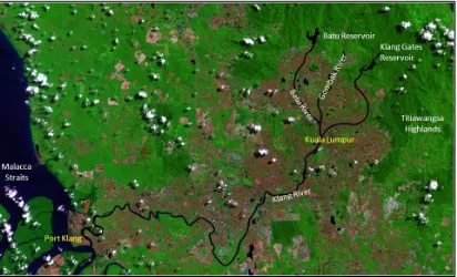
Kuala Lumpur is located in the eastern part of the Klang River basin (total area: 1278 km2_{). The} Klang, Gombak and Batu rivers originate in the densely forested foothills of the Titiawangsa mountain range, north of Kuala Lumpur and have their confluence near the old city centre, see Figure 4. The Klang river then continues its journey through the relatively flat and heavily urbanised valley floor before discharging into the Melaka Straits at Port Klang (Rustam, et al., 2000).

(14)

The Klang basin has a tropical climate with abundant rainfall of 2700 mm per year. The maximum precipitation occurs in October and November and in April, coinciding with the southeast and southwest monsoon seasons respectively (Rustam, et al., 2000). Rainfall is also the primary source of the basin’s two main drinking water reservoirs (Klang Gates reservoir and Batu reservoir).

Tin ponds are one of the most important hydrogeological features in Kuala Lumpur. Limestone, being easily erodible traps mineral deposits (especially tin) in its extensive networks of

fractures, conduits and cavities. Tin deposits were mined from the 1850’s until the 1980’s in open-cast mines. These mines have since been closed and flooded, creating Kuala Lumpur’s characteristic tin ponds (Yin, 1986). Because of the high permeability of the limestone, the tin ponds play an important role in regulating Kuala Lumpur’s water balance, providing water storage during heavy rains and being a major source of groundwater recharge. The

groundwater table in the valley is quite shallow at around 5 m below the surface, making it sensitive to pollution (Binnie dan Rakan, 1980).

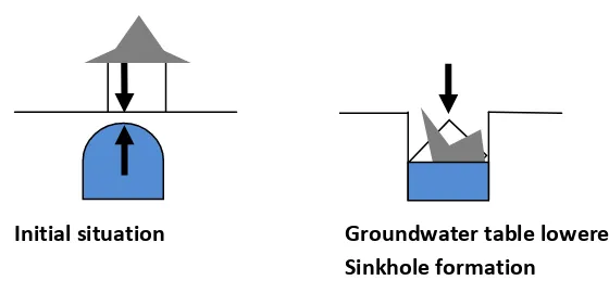
The irregular limestone formations also pose geotechnical engineering challenges. If groundwater levels fall and cavities and tunnels are drained, this can lead to sudden

catastrophic land subsidence (sinkhole formation) as illustrated in Figure 5. The sudden loss of support provided by the groundwater has caused the collapse of buildings in the past. Often these occurrences were related to the draining of tin mines or major construction projects (Tan, 2006).

Figure 5 – Simplified illustration of sinkhole formation mechanism.

Other geotechnical challenges are posed by the steep hills that surround most of Kuala Lumpur. Some of these hills have been cleared from natural vegetation to make way for development. Here, heavy rains occasionally induce landslides, some of them involving loss of life (LESTARI, 1997). These landslides are usually caused by inadequate local drainage which causes the soil to become saturated and lose its carrying capacity. However it is a very local problem, whereas sinkholes can be induced by groundwater extractions hundreds of metres away (Tan, 2006; Craig, 1997).

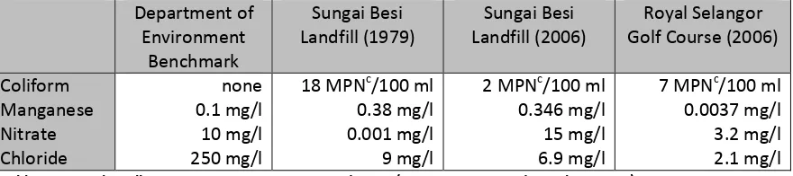
And then there is groundwater quality. Department of Environment monitoring reports indicate that groundwater quality in Kuala Lumpur is generally good, except near landfill sites where the manganese concentration exceed the Department of Environment benchmark. Manganese is a

Initial situation Groundwater table lowered

(15)

heavy metal commonly found in batteries and other chemicals. Manganese leaching is a known problem and has been reported at least since the 1980’s (Binnie dan Rakan, 1980). Leaching in tropical climates is often more severe than in temperate climates because heavy rainfall generates more effluent from landfills. Some sample groundwater pollutant concentrations are given in Table 1.

Water quality in the tin ponds is not monitored by the Department of Environment, but casual observation suggests that the water quality fairly good because many of the ponds are popular fishing spots used by local residents.

Department of

Table 1 – Sample pollutant concentrations in groundwater (JAS, 2007; Binnie dan Rakan, 1980).

2.3.2 Hydrogeology

The primary source of hydrogeological data is the Department of Minerals and Geoscience. At its offices in Shah Alam, the department has a library of borehole records which are mainly

collected from site investigation reports produced by private contractors. Location,

groundwater depth and bedrock depth data are available for 1305 points in the study area. Most data has been collected after 1980 (see Figure 6). The Department of Minerals and Geoscience also publishes maps that show the approximate boundaries of geological formations, fractures and the local top soils.

Figure 6 – Measurement points (red dots) and the extent of the study area (red line).

c

(16)

Detailed digital topographic maps (e.g. the L808 series) are available from the Department of Surveying and Mapping. These are used to identify the location of rivers and lakes. A digital elevation model is obtained from Shuttle Radar Topography Mission data made available on-line by the United States’ National Geospatial-Intelligence Agency and National Aeronautics and Space Administration. The digital elevation model is used in the groundwater model instead of the elevation data from the 1305 borehole records because the borehole data does not cover the entire study area.

Almost all of the borehole data is from the valley floor because most construction projects (and therefore most geotechnical investigations) take place there. The borehole data is only

representative for a very small area. Given the known large geological variation, errors can easily occur if a single measurement is assumed to be representative for large area, which happens if no other data points are available.

Borehole elevations can diverge by more than 50 m compared to the value assigned to the matching digital elevation model cell. Given that the total elevation range is more than 1000 m, this is an error of about 5%. Nevertheless, 50 m is significant considering that most

measurements are taken within the range of 0 to 100 m (Figure 7) and that cell dimensions are about 227 m × 227 m. However, given that there are 1305 borehole points and more than 10,000 cells, it is assumed that the error of the final model and calibration will average out and be smaller.

As mentioned earlier, the borehole data does not cover the entire study area, yet the model does require inputs for the entire study area. Therefore it is necessary to interpolate. There are basically two possibilities: spatial interpolation (e.g. kriging) and interpolation correlating to a variable that is available for the entire study area, in this case: elevation from the digital elevation model.

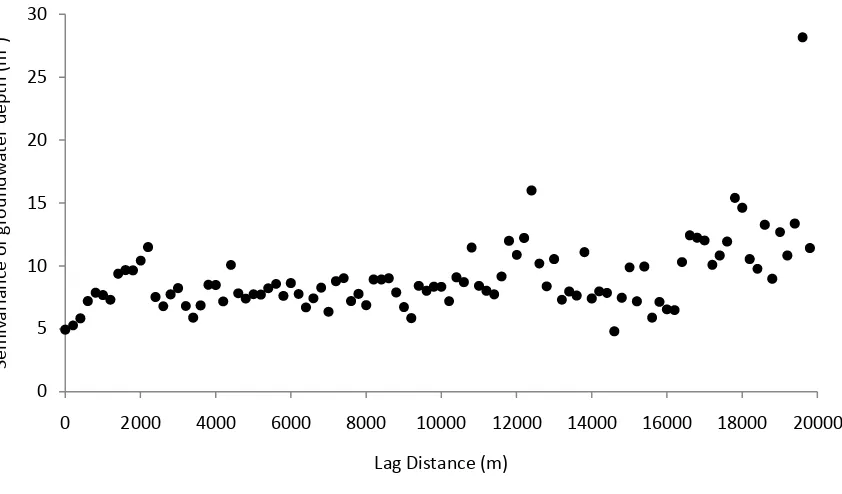
The spatial correlation of groundwater levels can be tested using a semivariogram (Figure 8). Alternatively, the relationship between groundwater levels and elevation can be plotted (Figure 7). Both graphs show clear results: there is no spatial correlation in the groundwater depth, but there is a clear linear relationship between groundwater levels and elevation.

Figure 7 – Plot of Elevation vs. Groundwater Levels for 1305 data points.

y = 0.989x + 3.648

(17)

Figure 8 – Semivariogram showing the lack of spatial correlation between groundwater depths.

The lack of spatial correlation between groundwater depths can be explained by the highly variable hydrogeology and measurement errors which can distort weak spatial trends. This can make the strong linear relationship between groundwater levels and elevations seem surprising. However the relationship between groundwater levels and elevation is offset by 3.65 m, which is essentially the average groundwater depth. Hence both conclusions do not conflict.

This still leaves the question of the validity of the linear relationship between groundwater levels and elevation. The relationship is based on data with an elevation of 0 to 250 m above mean sea level, yet this relationship must be extrapolated to elevations of up to 1400 m above sea level, for which no borehole data is available. One would expect the groundwater table to be deeper in the hills (higher elevations) and shallower at the valley floor (lower elevations). The available data does not show this trend.

Additionally, if tin ponds play a significant role in regulating the groundwater table, one would expect this to show in the groundwater data. But even if distance to a tin pond is plotted against groundwater depth, no such relationship is evident (graph not shown).

Nevertheless, the relationship between groundwater levels and elevation is clearly

demonstrated at the valley floor. The valley floor is the main focus of the groundwater flow model because the hydrogeological formations that have most groundwater potential are located there. Therefore the groundwater level inputs for the model are generated from the digital elevation model while the comments made in this section must be taken into account when interpreting the model results.

2.3.3 Water Balance

Hydrological data for the water balance is obtained from the Department of Irrigation and Drainage maintains an extensive network of river discharge, reservoir level and rainfall

measurement stations. Unfortunately the measurement series of many stations are incomplete and unreliable. Aggregated data about water supply, leakage and consumption are available

0

0 2000 4000 6000 8000 10000 12000 14000 16000 18000 20000

(18)

from the Selangor Water Supply Corporation and the Malaysian Water Association. Evaporation data is obtained from a Landsat image made available by the Global Land Cover Facility of the University of Maryland.

The purpose of setting up the water balance is to generate inputs for the model, to gain insight into the quantity of water flowing through the study area and to fill gaps for which no

measurements are possible or available (e.g. infiltration). The water balance is split in three parts: above ground, piped water and groundwater, which are all linked to each other .

These links and relevant assumptions are explained in the next few paragraphs, as well as how model inputs are distilled from the water balance data. The water balance is calculated for the area upstream of the Klang River discharge gauging station at Sulaiman bridge. (Sulaiman bridge is roughly located at the ‘Kuala Lumpur’ label in Figure 4) The water balance area is 414 km2_.

Water Balance A (Above Ground)

ID Term Amount (mm/yr) Source

Tap water (flowing out from pipes, P2) Water intake (being put into pipes, P1)

+2792.9

Dept. of Irrigation and Drainage Landsat image

Calculated from water balance Dept. of Irrigation and Drainage Malaysian Water Association

Water intake (from surface water, A6) Tap water (to consumers, A5)

Loss (to groundwater, G2)

Net export/import (from outside area)

+245.6 Calculated from water balance

Water Balance G (Groundwater)

ID Term Amount (mm/yr) Source

G1 G2 G3

Recharge A (from above ground, A3) Recharge P (from leaking pipes, P3) Deep groundwater discharge

Calculated from water balance

Evapotranspirationd_{(A2) is an important factor in the water balance, in this case being}

equivalent to 43% of rainfall, the main source of water. Evapotranspiration is calculated from a Landsat image taken over Kuala Lumpur in 2001 (GLCF, 2001) using the Surface Area Balancing algorithm (Bastiaanssen, et al., 1998). This algorithm requires several additional inputs such as emissivity. An atmospheric correction must also be performed (Iqbal, 1983).

Since no atmospheric data for Kuala Lumpur are easily available, atmospheric data for a clear day from the National University of Singapore observation station is used. Given the geographic proximity of both cities and similar climates and levels of economic development (and air pollution), Singapore data is deemed an acceptable surrogate. Atmospheric data from Singapore

d

(19)

is made available on-line by the National Aeronautics and Space Administration’s Aerosol Robotic Network (AERONET, 2007).

An estimate for emissivity is based on published field work results from a study conducted in African cities. Emissivity mainly depends on the material, temperature and geometry of the object, in this case a city. The city of Dar Es Salaam in Tanzania is most similar to Kuala Lumpur in terms of climate and economic development compared to the other African cities included in the study. The emissivity parameter value used for Dar Es Salaam is 0.8. Emissivity in the heavily built-up and congested city centre and the city’s green outskirts is both approximately 0.8 on average, although it varies by about 0.05 throughout the day (Jonsson, et al., 2006). The calculated evapotranspiration ranges between 0 and 2.72 mm/hour, which is high but not impossible for an instantaneous observation made on a clear and hot day. Average pan

evaporation for Kuala Lumpur is 1606 mm/year (4.4 mm/day) (CTI, et al., 2001). Pan

evaporation is the maximum possible evaporation. The hourly evaporation is scaled to a daily evaporation that ranges from 0 to 4.4 mm/day.

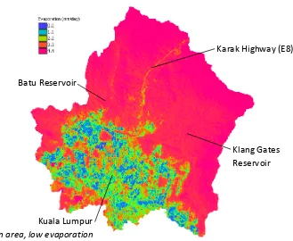
A single satellite observation is not suitable for calculating average evaporation, but here it is used to estimate relative evaporation between different types of land cover (e.g. urban and vegetation). The scaled average evaporation is 3.29 mm/day (used in the water balance), it is about 1 mm/day in urban areas. The distributed evaporation for the water balance area is given in Figure 9.

Figure 9 – Evaporation map of water balance area.

Water intake capacities (A6) for the water balance area are displayed on the website of the Selangor Water Supply Corporation. The intake locations included in the water balance (above

Kuala Lumpur urban area, low evaporation

Klang Gates Reservoir Batu Reservoir

(20)

ground) are Bukit Belacan, Taman TAR, Klang Gates Reservoir and Batu Reservoir (the latter two reservoirs are indicated in Figure 4). It is assumed that water use is broadly constant so that water intake and water intake capacity are similar.

The water consumption (A5) and pipe leakage (P3) data are from the Malaysian Water Association (MWA, 2006). The Malaysian Water Association provides lumped data for all of Kuala Lumpur, Selangor and Putrajaya combined. To estimate consumption and leakage in the water balance area, it is assumed that population correlates closely to consumption and leakage. Although consumption patterns between residential areas and industrial areas differ, within the study area there are both large residential areas (e.g. Wangsa Maju) and industrial areas (e.g. Gombak) and so the assumption is expected to hold. The census districts of Gombak, Selayang, Wangsa Maju, Sentul, Damansara and Kuala Lumpur City Centre are located in the water balance area. According to the 2000 census 1.3 million people live here. This is 26% of the total population of Selangor, Kuala Lumpur and Putrajaya. Agricultural water use in the Klang basin is negligible because the vast majority of the agricultural acreage is used for oil palm

plantations, which are not irrigated.

The Malaysian Water Association also provides statistics on non-revenue water. If we assume that the water balance area follows the national average, then 50% of non-revenue water is leaked and the other 50% of non-revenue water is unmetered (Sakura, et al., 2006). Therefore the water consumption in the water balance area is estimated at 218 million m3_{/year and total} leakage is 68 million m3_/year.

Groundwater recharge (or infiltration, G1 & G2) is an input for the groundwater model and it is calculated using the water balance. Being the remainder of the balance, it includes all infiltration from rainfall and pipe leakage. But there is an additional, secondary source of infiltration which is not accounted for in the water balance: water used by consumers which is not evaporated and does not reach the surface water can infiltrate into the ground, possibly posing a pollution threat. 70% of Kuala Lumpur residents are connected to the central sewerage system so the amount of secondary infiltration is likely to be quite small. Note that wastewater treatment facilities are also small, serving their local surroundings and hence they are located within the water balance area (DBKL, 2000) and thus accounted for in the water balance.

This relatively small secondary source of infiltration is very difficult to measure or calculate and therefore it is ignored at this time. Given that the purpose of the groundwater flow model is to estimate groundwater extraction potential, ignoring secondary infiltration will likely lead to a slight under-estimation of the groundwater potential. This is a prudent course of action because extracting too much groundwater (overestimating the potential) is far more damaging than extracting too little (underestimating the potential).

(21)

and is calculated at a rate of 4,369 mm/year, which is deemed realistic as it is just a fraction of the theoretical hydraulic conductivity of the fractured limestone in which the ponds are located.

2.4

Model Setup and Calibration

Following the model selection and data analysis in the previous sections, in this section the model setup and calibration are addressed. To begin, the model schematisation and some important modelling choices are explained along with a description of the parameters and variables. This is followed by the calibration process, calibration results and some general observations about the model performance.

The famous physicist Albert Einstein once remarked that we should “make everything as simple as possible and as complicated as necessary,” a point that is very valid in groundwater

modelling too. There are four important modelling choices which rely on certain simplifications and assumptions which must be clearly explained if the model and model results are to be fully understood. In the next paragraphs the choice of model boundaries, the assumption of steady-state flow, cell size (model resolution) and the choice between a single layer and a double layer model are all addressed.

The boundaries of the groundwater model generally follow the hydrological boundaries because the hydrogeology also follows the direction of hydrological flows and there are no good measurements that allow the definition of other boundaries. The more permeable

hydrogeological formations, Kuala Lumpur Limestone and Kenny Hills, are located under the valley floor, while the surrounding hills are underlain by more impermeable formations such as Hawthornden and Granite (Figure 2). These ‘hydrological’ boundaries are modelled as no-flow boundaries. Where there is an absence of hydrological boundaries, a constant head boundary is imposed based on the interpolated groundwater level data. Most of these constant head

boundaries are located on the valley floor, an area for which more data is available.

The model is assumed to be steady-state (inflow is equal to outflow at every time-step). This assumption is necessary because it allows the use of groundwater data from different locations and different times. Although desirable, a steady-state model does not require continuous groundwater level monitoring time series, unlike a transient model. Because there are very few artificial groundwater extractions in the study area and mining activities seized in the 1980’s the system is probably close to steady state. Casual observations suggest that water levels in the tin ponds are constant. Given their role in regulating the groundwater level, groundwater levels are also assumed to be constant. No measurements are available that can confirm or reject this assumption.

The Equivalent Porous Medium method holds that the cell-size should be sufficiently large so that the highly irregular medium behaves like a regular, porous medium when modelled. However, by assigning a single hydraulic conductivity parameter to an entire hydrogeological formation, the model becomes lumped, already satisfying the Equivalent Porous Medium method. Cell-size is instead determined by the calculations speed and the geographic variability of the study area. Large cells speed up calculations, but excessively large cells that aggregate data for large areas distort model characteristics such as elevation and infiltration.

(22)

much. The choice of cell dimensions is a li

optimisation were made once the model calculation time was found to be sufficiently short (around 30 seconds) and the input seemed sufficiently detailed. The model grid consists of 187 rows and 137 columns.

Finally: the decision to construct seem to sustain a double layered

granite, schist) can be identified overlaid by an upper layer

deposits, a layer with a thickness of between 0 and 80 m. To quantify flow between MODFLOW requires the introduction of a leakance term. There is no data that suggests impermeable or less permeable

value must be assigned to simulate flow between both layers, effectively making the model a dual porosity medium, a concept discussed in

Because of calibration difficulties, which model is calibrated. The single

bedrock layers is not known, but it is assumed that 300 m is sufficiently deep for groundwater flows to be minimal so that the hydraulic conductivity calibration can be performed

successfully. It must be noted that the calibrated hydraulic conductivity

thickness, but this is not a problem as long as the layer thickness is kept constant during simulations.

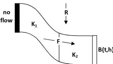
The model schematisation is shown in

Input

R = Recharge (m/day) – input

Parameters

K = Hydraulic conductivity (m/day) B = Hydraulic boundary

t = transmissivity (m2/day) – estimated h = head on boundary (m) – estimated Specific yield and specific storage

K1

Figure 10 – Model schematization (side view).

much. The choice of cell dimensions is a little arbitrary and no efforts at further cell

optimisation were made once the model calculation time was found to be sufficiently short (around 30 seconds) and the input seemed sufficiently detailed. The model grid consists of 187

Finally: the decision to construct a single layer or a double layer model. At first sight, the data ed model because a lower rock formation (limestone, sandstone, granite, schist) can be identified overlaid by an upper layer of weathered rock

, a layer with a thickness of between 0 and 80 m. To quantify flow between MODFLOW requires the introduction of a leakance term. There is no data that suggests

or less permeable zone separates both layers. Therefore a very high

mulate flow between both layers, effectively making the model a dual porosity medium, a concept discussed in Section 2.2.

Because of calibration difficulties, which are discussed later in this section, only a single layer layer is 300 m thick. This is because the exact depth of t

bedrock layers is not known, but it is assumed that 300 m is sufficiently deep for groundwater flows to be minimal so that the hydraulic conductivity calibration can be performed

successfully. It must be noted that the calibrated hydraulic conductivity is affected by the layer thickness, but this is not a problem as long as the layer thickness is kept constant during

is shown in Figure 10 and Figure 11.

K = Hydraulic conductivity (m/day) – calibrated

estimated

Specific yield and specific storage – literature values (Anderson, et al., 1992) B(t,h)

Inactive cells

Active cells

Direction of flow

Figure 11 – Model schematisation (top view). Model schematization (side view).

ttle arbitrary and no efforts at further cell-size optimisation were made once the model calculation time was found to be sufficiently short (around 30 seconds) and the input seemed sufficiently detailed. The model grid consists of 187

model. At first sight, the data (limestone, sandstone, of weathered rock and alluvial , a layer with a thickness of between 0 and 80 m. To quantify flow between two layers, MODFLOW requires the introduction of a leakance term. There is no data that suggests that an

herefore a very high leakance mulate flow between both layers, effectively making the model a

are discussed later in this section, only a single layer . This is because the exact depth of the bedrock layers is not known, but it is assumed that 300 m is sufficiently deep for groundwater flows to be minimal so that the hydraulic conductivity calibration can be performed

is affected by the layer thickness, but this is not a problem as long as the layer thickness is kept constant during

Active cells

(23)

Variables

Groundwater head (m) – input (initial), then calculated F = Horizontal flow (m3/day) - calculated

Output

Deep groundwater discharge (m3/day) – calculated

Setting the hydraulic boundary requires the constant head and the transmissivity to be

specified. The transmissivity is not a very sensitive parameter and is set large enough so that it does not form a barrier to the deep groundwater discharge. The constant head is taken from the interpolated groundwater levels. The groundwater model is quite sensitive to the constant head parameter. Recharge is also a very sensitive parameter, which is not surprising, given that it is the input. The hydraulic conductivity of the Kenny Hills and Kuala Lumpur Limestone are also sensitive parameters. This can be explained by the fact that in these areas more recharge takes place, so any changes have a significant impact on the water table.

The calibration is done through a mix of UCODE, PEST and trial-and-error to find a set of hydraulic conductivity parameters which are within the range of expected literature values (Anderson, et al., 1992; Scanlon, et al., 2003), which have appropriate values relative to each other (e.g. granite should be less permeable than sandstone, etc.) and which ensure a closed water balance, a pre-requisite for any steady-state calibration. Obtaining such a set is not very easy as there are many optima which satisfy at least some of these conditions. The optimisation codes try to minimise the discrepancy between the measured and simulated water table for 9 calibration points and this does not necessarily coincide with a closed water balance or realistic values.

It could be argued that 9 calibration points are too few, especially considering there are more than 1305 data points available. However these 9 points have elevations that closely match the digital elevation model (error less than 1 m), making them very reliable. In addition, they have a good spatial distribution. Calibrations with more calibration points were also attempted, but these often created one or two ‘trash calibration points’ which had exceptionally large errors and still produced unrealistic calibration results. This leads to the decision to calibrate with 9 well distributed, high quality points only.

The reason for the calibration problems are probably the interdependence of the parameters. To improve the calibration, the granite and schist formations are lumped together because their hydraulic conductivities, specific yield and specific storage are very similar. This reduces the degrees of freedom in the calibration. This is also the reason why only a single layered model is calibrated and not a double-layered one. So the hydraulic conductivities of just three formations are calibrated: Kuala Lumpur Limestone, Kenny Hills and Granite/Hawthornden. The results are presented in Table 2.

Formation H.Conductivity (m/day) Specific Yield* Specific Storage* (m-1)

K.L. Limestone

(24)

It must be noted that the calibration faces the problem of equifinality: there are other solutions that satisfy the calibration conditions. But how significantly do these results differ from the calibration results presented here? This question could be resolved by testing a different set of calibrated hydraulic conductivity parameters and seeing if the model output is very different. Sensitivity analysis suggests that this will not be the case, unless the hydraulic conductivity parameters are changed significantly. In that case they would violate the calibration conditions. Therefore equifinality is not explored further at this time.

The error in the water balance calibration is less than 0.01%. The root mean square error of the calibrated water tables compared to the measured values is 13.4 m. Considering that the total difference in groundwater levels within the study area is 1472 m, this is an error of 0.91%. These statistics alone do not give a full picture of the calibration results. If simulated points not included in the calibration are compared to the measured and interpolated values there are very large discrepancies. Figure 12 shows that errors in hilly areas (red area) exceed 50 m and in some cases are as large as 250 m. It is interesting to note that the simulated groundwater depth does show clear spatial correlation and lacks a clear relationship between elevation and groundwater levels: the exact opposite of the conclusions drawn from the data in Section 2.3.2.

(25)

It must be concluded that the final calibration results are mixed. There is a clear mismatch between the interpolated data and the simulated data. If a choice is made between the two ‘possibilities’, the simulated data seems most reasonable given that it shows the expected spatial correlation in groundwater depth. Yet this mismatch does introduce a large degree of uncertainty into the model.

However the water balance is calibrated correctly and the calibration error for the groundwater table at the valley floor, the focus of the model, is reasonably small. Note that the specific yield, storativity and recharge (see Section 2.3.3) are conservatively estimated. This slightly

underestimates the groundwater potential, which is appropriate as groundwater potential overestimation can be very damaging.

Therefore one can conclude that the calibrated model provides a good estimate of the quantity of groundwater available at the valley floor, but it does not offer any certainty as far as

predicting flow directions or specific groundwater levels are concerned.

2.5

Evaluation of Extraction Strategies

Due to model limitations, the range of extraction strategies that can be tested is somewhat limited. For example, the model calibration does not inspire enough confidence to be able to confidently predict the water table and flows at a specific location. Nevertheless, given that the water balance of the model is sound, it is possible to make a rough estimate of the quantity of groundwater that can be extracted. This figure, capturing the potential size of Kuala Lumpur’s groundwater resources, is of economic and policy significance.

To evaluate the extraction strategies, relevant criteria need to be determined. Although there is basic knowledge about potential geohazards in Kuala Lumpur, there is little hard data that can be used to quantify these criteria. In this section simple quantitative criteria are used, although the process of setting them is somewhat arbitrary. This is followed by the evaluation of two generic extraction strategies: permanent extraction and temporary extraction. First the effects of a local extraction (single well) is considered. Then the effects of a macro extraction (multiple wells) are simulated.

Common costs of groundwater over-extraction are:

1. Extraction costs such as well drilling, pump installation, maintenance and power. Over-extraction can lower the groundwater level, increasing Over-extraction costs.

2. Over-extraction can lead to a decrease in spring discharge, base flow and lake volume which may adversely affect the natural environment.

3. Groundwater flow patterns can change with potentially detrimental effects to groundwater quality, e.g. infiltration through polluted soil can increase.

4. The decline in pore water pressure may lead to land subsidence, or in fractured limestone areas to sink-hole formation (Custodio, 2002).

(26)

Prior to the 1980’s when the tin mines still operated, local groundwater drawdown at mines of 20 m or more was not uncommon and therefore this is a kind of benchmark for the Limestone aquifers, where the tin mines (now tin ponds) are located. We assume that there is no threat of sinkhole formation for buildings built before 1980, if there was, they would have already collapsed. We also assume there is no threat for newer buildings: they should have complied with a modern building code. Therefore we assume that a global 5 m drawdown will not trigger any sinkhole formations and is acceptable in the case of an emergency and if adequate

environmental protection measures are taken.

In MODFLOW groundwater extraction wells are simulated as a ‘sink term’ or ‘loss term’ from a cell. It is suggested that 8,000 m3_{/day is a reasonable pumping capacity for wells in the}

limestone aquifer (LESTARI, 1997), so hence a well field in a cell with an area of 5 ha may well contain 10 wells and thus a total well field capacity of 10 x 8,000 = 80,000 m3_/day.

These wells can be used to extract water permanently or temporarily, say during a period of 100 days (approximately three months) during a drought followed by a period of 1000 days (approximately three years) during which the groundwater table can recover. During a short period of extraction, presumably more groundwater can be extracted. Additionally, extractions from a single well field are likely to have a smaller impact than extractions from an entire well field. This leads us to four scenarios, see Table 3.

Scenario Extraction per well field (m3/day) Number of well fields Duration P1

T1 P2 T2

800 / 8,000 / 80,000 80,000

8,000 80,000

1 1 12 12

Permanent 100 days Permanent 100 days

Table 3 – Extraction scenarios.

The purpose of Scenario P1 is to see which permanent extraction is feasible, considering 80,000 m3_{/day is the maximum possible extraction. The purpose of Scenario T1 is to see how rapidly} the groundwater table recovers. The results from both scenarios are given in Figure 13.

(27)

Figure 13 – Scenario P1 (single well permanent extraction, left) and Scenario T1 (single well 100 day extraction, right).

To test the impact of large scale extractions (12 well fields), scenarios P2 and T2 are simulated. Scenario P2, with a total permanent extraction of 96,000 m3_{/day reaches a stable drawdown of} 1 m after 1500 days of simulation. Scenario T2, with a total temporary extraction of 960,000 m3_{/day reaches a maximum drawdown of 5 m and is almost fully recovered within the 1000} day period. The evolution of the groundwater table in Scenario T2 is shown in Figure 14.

Figure 14 – Scenario T2 with large scale temporary extraction.

Both large scale extraction strategies that were simulated (scenarios P2 and T2) met the simple quantitative criteria that were set. This basically suggests that there are two extraction

strategies possible: permanent extraction of 96,000 m3_{/day and a temporary extraction of} 960,000 m3_{/day continuously during 100 days.}

(28)

These conclusions are tentative because there are some problems with the model calibrations as explained in the previous section that must be appreciated. Definitive conclusions about the appropriate extraction strategy can only be drawn once a more thorough groundwater study has been conducted and certain important model assumptions, such as the model’s steady state condition and the groundwater table in hilly areas, are verified.

(29)

3

Governance of Groundwater Resources

3.1

Introduction

Former United Nations Secretary General Boutros Boutros-Ghali once said that “the best way to deal with bureaucrats is with stealth and sudden violence.” It seems Boutros-Ghali held a rather glum view of bureaucracies, yet he would probably agree that we should first do an institutional analysis (‘stealth’), so that we know how to use ‘sudden violence’ to implement a sound

groundwater policy, in doing so answering the research question: What is the current institutional setting with respect to groundwater resource management and how can it be changed to enable groundwater extraction?

An understanding of the institutional setting is important, especially in the field of integrated water management where problems are often complex and poorly defined because knowledge is incomplete and policy actors can have different problem-perceptions and competing

interests. By ignoring the institutional feasibility, one risks developing an irrelevant (technical) solution that simply will not be implemented.

Having established the purpose and necessity of an institutional analysis, this brings us to selecting a framework for performing the institutional analysis. But which analytical framework is suitable for evaluating the institutional setting? And, more importantly, how can this

framework lead to useful conclusions and recommendations? Given that governance has strong local characteristics, the framework must be able to perform under different water management regimes in different countries.

Bressers et al have developed an institutional analysis framework for comparing water resource management regimes in different countries and identified Policy Coherence as the key criterion for successful and sustainable water management based on an extensive review of European and American literature on natural resource governance. Furthermore, Bressers et al

successfully applied their method in six European countries including France, Spain, the

Netherlands and Switzerland which all have very different histories and systems of governance (Bressers, et al., 2003).

Although the Policy Coherence framework was developed for and applied in six continental European countries, the ideas on which it is based find wide application elsewhere, including in the United States and the United Kingdom. Given that the Malaysian government and legal system are modelled on that of the United Kingdom, it is reasonable to assume that the Policy Coherence framework can also be applied to groundwater management in Kuala Lumpur. In this chapter, the Policy Coherence framework is explained (Section 3.2) and then applied by performing the institutional analysis (Section 3.3) and identifying conditions for policy

coherence (Section 3.4). Based on this analysis, some institutional changes are explored that might enable groundwater extraction (Section 3.5).

3.2

Analytical Framework

(30)

necessary to carry out sustainable water policies. Policy coherence cannot be imposed because there is no policy actor that has full control. Even a powerful government agency will need to respect property rights, legal jurisdictions and prevailing interests (Bressers, et al., 2003).

Bressers also observes that there are several key barriers to making groundwater policy that leads to a win-win situation or profitable trade-offs between policy actors. Uncertainty, along with the problem’s complexity, the long-term time-scale of groundwater changes and pluralism (i.e. the presence of multiple policy actors) can prevent effective decision-making (Bressers, et al., 2003). And while the previous chapter attempted to reduce uncertainty through modelling, this chapter focuses on how cooperation between multiple policy actors can be stimulated. The other plank of Bressers’ research concerns water use rights. However this topic is not very relevant to this specific study because the property and use rights of groundwater are very simple. In Kuala Lumpur groundwater use rights are regulated by a single agency and current groundwater use is insignificant.

In analysing policy coherence, Bressers also stresses the need to identify and take into account that decision-making happens at many levels and that these decisions influence each other.

The institutional analysis is conducted by answering a list of questions that cover all the elements of the Policy Coherence framework: levels of governance, policy actors, perceptions and objectives, policy instruments and resources. The conditions for policy coherence identified by Bressers et al are: a tradition of cooperation, joint problems, joint opportunities, the

presence of a credible alternative threat and institutional interfaces (Bressers, et al., 2003).

3.3

Institutional Analysis

The institutional analysis is structured along the elements of Bressers’ governance model (policy instruments and resources are combined under a single heading). Detailed questions for each element are given in Appendix A.

Levels and Scales of Governance

Malaysia is a federation in which state governments have significant autonomy. Under article 73 of the federal constitution, state governments have jurisdiction over water and land resources, whereas the federal government can legislate on interstate issues such as pollution control, mining and public health (Perunding Zaaba, 1999). A complete listing of all organisations involved in Kuala Lumpur’s groundwater management is given in Table 4.

Selangor state has created a single agency, the Selangor Waters Management Authority, to manage its key responsibilities in the fields of water resources and water supply. In Selangor and Kuala Lumpur the water supply system is operated by the Selangor Water Supply Corporation, a private company which has a concession granted by the Selangor state

government and which is part-owned by the Selangor State Investment Company: Kumpulan Darul Ehsan Berhad.

(31)

Planning Department is responsible for land-use planning at the national and state levels, which includes gazetting sensitive riparian areas and groundwater recharge zones.

Federal Agencies

Ministry of Natural Resources and Environment

• Department of Environment

• Department of Minerals and Geoscience

• National Hydraulic Research Institute Malaysia Ministry of Federal Territories

• Kuala Lumpur City Hall

Ministry of Energy, Water and Communications

• National Water Services Commission Treasury (Ministry of Finance)

• Water Asset Holding Company

Ministry of Health

Federal and State Agencies

Ministry of Natural Resources and Environment

• Department of Irrigation and Drainage Ministry of Housing and Local Government

• Town and Country Planning Department Ministry of Public Works

• Department of Public Works

Selangor State Agencies

Selangor Waters Management Authority

Kumpulan Darul Ehsan Berhad (Selangor State Investment Company) Local Authorities of Selangor State such as Ampang Jaya Municipal Council, Petaling Jaya City Council, etc.

Private Companies Selangor Water Supply Corporation

Table 4 – Overview of organisations dealing with groundwater in Kuala Lumpur.

The Selangor Water Supply Corporation, being a private water utility, is regulated by the federal government’s National Water Services Commission. The Commission regulates water prices, piped water quality and water delivery. The Selangor Water Supply Corporation buys water from water treatment plants which are operated by other companies. Some of these plants are privately owned, others are owned by the state government or the federal government’s Water Asset Holding Company. Because the Selangor Water Supply Corporation supplies drinking water, it is also supervised by the Ministry of Health which operates small-scale water supply projects in some rural areas, but not in Kuala Lumpur.

The Department of Irrigation and Drainage, the Department of Public Works and the

Department of Town and Country Planning are federal departments but the state governments hold significant powers over their state-level operations. The Department of Environment and the Department of Minerals and Geoscience are pure federal agencies who assist state

governments but are not controlled by them.

Local authorities such as Kuala Lumpur City Hall are required to monitor development in Environmentally Sensitive Areas and withhold building permits if it is deemed prudent to do so. (LESTARI, 1997) Local authorities fall under the control of the state government (there are no local elections), and in the case of Kuala Lumpur, which is a federal territory, under the Ministry of Federal Territories.

(32)

required to supply water (a duty carried out by the Selangor Waters Supply Corporation) but it has no jurisdiction over the city’s water resources.

Research on water management issues is conducted by the National Hydraulic Research Institute Malaysia, an institute of the Ministry of Natural Resources and Environment. An overview of the abovementioned agencies is given in Table 4.

The Malaysian government is legalistic and hierarchical. This can prevent cooperation between different levels of government. This legalistic nature of the government is evident from the following example about groundwater monitoring activities. The Department of Environment monitors groundwater quality as part of its tasks to control pollution under the Environmental Quality Act (1974). The Department of Minerals and Geoscience monitors groundwater levels because it has to study hydrogeology as instructed by the Geological Survey Act (1974). This leads to the peculiar situation where both departments operate completely separate

groundwater monitoring networks. At Department of Environment wells only groundwater quality is measured. At Department of Minerals and Geoscience wells only groundwater levels are measured. However both departments fall under the same Ministry of Natural Resources and Environment.

In terms of hierarchy, federal ministers and state chief ministers have roughly the same level of authority. So for a comprehensive groundwater policy to be initiated in Kuala Lumpur, the chief minister of Selangor and eight federal ministers must reach agreement. This fragmentation of authority makes regulation of water resources in Malaysia ineffective (Zakaria, 2001; Madsen, et al., 2003; Mutadir, 2006; BERNAMA, 2007).

Only the Prime Minister, backed by the federal parliament and the treasury, has a higher standing than the federal ministers and the chief ministers. The Economic Planning Unit of the Prime Minister’s department establishes 5-year plans which direct policy for all ministries and state governments. The current 5-year plan (2006-2010) is the Ninth Malaysia Plan.

Historically, the federal government and the state governments have been controlled by politicians from the National Front coalition. However following the 2008 general elections the National Front lost power in Selangor to the People’s Front coalition. Therefore the position of the Prime Minister in relation to the Chief Ministers is likely to change in future.

Actors in the Policy Network

Under the Ninth Malaysia Plan increased groundwater extraction is seen as one way of expanding Kuala Lumpur’s water supply, in addition to water conservation and an inter basin water transfer scheme. The relevant government agencies have already been mentioned in the previous sector. In this section their roles with respect to groundwater management are further specified and other relevant actors are introduced.

(33)

The reality is very different: Dr. Lim Keng Yaik, Minister for Energy, Water and Communications first proposed in the media that groundwater resources be “fully utilised” to supplement

existing sources of water supply (BERNAMA, 2007). He also mentioned that he was briefed by the Selangor Water Supply Corporation and the Selangor State Investment Company about possible groundwater sources (Hamsawi, 2007).

This seems counter-intuitive, because the Minister for Energy, Water and Communications has no formal control over Selangor’s Water Supply Corporation or State Investment Company. However his ministry regulates the Water Supply Corporation through the National Water Services Commission which sets water tariffs, thus exerting significant influence. The Ministry of Energy, Water and Communications also manages the tender process for new water supply infrastructure and the Selangor State Investment Company bids on these projects (The Edge, 2007). Hence one must conclude that the Ministry of Energy, Water and Communications effectively controls the Selangor and Kuala Lumpur water industry.

There are also several non-governmental organisations that are critical of the governments’ current water policy for various reasons. They include the Malaysian Trade Union Congress which opposes privatisation of water utilities and the Malaysian Nature Society, the World Wildlife Fund, the Consumer Association of Penang and local academics such as Prof. Ir. Dr. Zaini Ujang of the University of Technology Malaysia who are concerned about the

environmental impact of government policies (Netto, 2005; BERNAMA, 2007; MNS, 2008).

In recent years the influence of public opinion on policy making has increased substantially. This is clearly demonstrated by the defeat of the government’s proposal to build an incinerator at Broga, near Kuala Lumpur, which was vehemently opposed by local residents. Before the plan could be challenged in court, the government withdrew its proposal (BERNAMA, 2007). Almost a decade earlier, following the 1998 water crisis, the government managed to push through the Selangor River Dam with little fuss, which was also highly controversial because of

environmental concerns (CAP, 1999).

Lastly, there are the water consumers. The vast majority of water is provided by the Selangor Water Supply Corporation, but it is supplied below cost (ADB, 2004). Domestic consumers in Selangor will receive the first 20 m3_{/month of water free from June 1}st_{2008 onwards. (Singh,} 2008) Due to the low cost of piped water and the poor quality of groundwater in Kuala Lumpur (it requires some treatment before it can be used for human consumption), there is very little groundwater extraction by consumers. However, private parties can apply for a license to extract groundwater from the Department of Minerals and Geoscience (in Kuala Lumpur) or the Selangor Waters Management Authority (in Selangor